Phytoplankton in transitional waters: Sedimentation and Counting methods

http://siba-ese.unisalento.it

Phytoplankton in transitional waters: Sedimentation

and Counting methods

C. Mazziotti1*_{, A. Fiocca}2_{, M. R. Vadrucci}3

1_{ARPA Emilia-Romagna - Regional Agency for the Environmental Prevention}

Viale Vespucci, 2, 47042 Cesenatico, Italy.

2_{Department of Biological and Environmental Sciences and Technologies,}

University of Salento Via Provinciale Lecce-Monteroni, 73100 Lecce, Italy.

3_{ARPA Puglia-Regional Agency for the Environmental Prevention and}

Protection, Department of Lecce, Via Miglietta 2, 73100 Lecce, Italy. *Corresponding author: E-mail address: cmazziotti@arpa.emr.it

Abstract

1 - The methodological issues in the analysis of phytoplankton guilds in transitional waters, using inverted microscopy (Utermöhl technique), will showing and discuss, in reference to UNI EN 15204, particularly regarding sedimentation and counting steps.

2 - The statistical processes for the validation of the two steps will showing and discuss

Keywords: method, homogenisation, phytoplankton, validation. RESEARCH ARTICLE

Introduction

Phytoplankton is a key ecological element of transitional aquatic ecosystems, through which energy flows are channelled. Microphytoplankton is made up of a group of autotrophic organisms of between 20 µm and 200 µm in diameter. They live in the water column and include both solitary and colonial forms. In transitional aquatic environments, phytoplankton plays a fundamental role in the formation of new organic substances and in recycling carbon, nutrients and oxygen. Phytoplankton is an excellent indicator of changes in the trophic state of the waters and of short-term impacts such as nutrient enrichment, which lead to increased biomass, primary production and algal blooms as well as changes in species composition. In addition, phytoplankton responds to

variations in chemical-physical parameters and hydrodynamics. Indeed, it has been demonstrated that variations in temperature and salinity induce variations in the community characteristics of phytoplankton corporations.

National and EU laws (Italian law D.Lgs. 152/06 and the EU's WFD 2000/60) have also identified phytoplankton as a biological quality element, since it seems to be a good indicator for assessing the state of health of transitional water ecosystems and Marine Coastal Waters (Ward and Jacoby, 1992). Here will examine and discuss sedimentation and counting methods using an inverted microscope (the Utermöhl technique) with reference to UNI EN 15204 “Water quality- Guidance standard on the enumeration of phytoplankton using inverted microscopy”.

ـ in each field all the algal cells discovered were counted;

ـ tests were performed to verify that the number of cells counted per chamber satisfied the criteria of the central limit theorem; ـ the Huber test was performed on the 10 fields per sedimentation chamber to eliminate any anomalous data;

ـ the chi-square test was performed on each sedimentation chamber to verify that the counting differences between the 10 fields were random (random distribution allows for simple and uniform counting strategies and statistical procedures to assess measurement uncertainty);

The results show the applicability of the Central Limit Theorem, the absence of anomalous data (negative in the Huber Test) and the chi-square values confirm the validity of the sample homogenisation (Table 1). 1.2 The sub-sample preparation was validated as follows:

ـ the chi-square test was performed on the counts obtained in the 12 sedimentation chambers in order to verify the plausibility of the null hypothesis, i.e. the randomness of the difference in counts observed in the 12 sedimentation chambers (p>0.05) (Table 2). During the process of sedimentation, shape, size, silicification and membership of colonies appeared to be the decisive factors in determining sedimentation rates.

The technique used to add the sub-samples to the counting chambers is crucial, as it affects the final distribution of settled particles. The chamber should be filled directly from the sample bottle. The exact volume depends on the phytoplankton density, the volume of the counting chamber and its surface-to-volume ratio. Larger sub-sample volumes (up to 100 ml) will be required from oligotrophic waters. At high phytoplankton density a dilution step may be necessary to ensure that the concentration of particles is sufficiently low to prevent excessive adhesion and to Currently the European Standard EN 15204

is the only method which is both complete and provides detailed guidelines.

The Utermöhl technique, using an inverted microscope, is the recommended method for analysing phytoplankton abundance and composition. This paper assesses sedimentation in round (tubular) chambers. Materials and methods

This study includes a review of a methodological approach. In order to perform the UNI EN statistical tests, a group of phytoplankton samples were taken from Goro Lagoon (Lat. 44.47703 WGS84 Long. 12.21109 WGS84) on June 21th 2008, fixed with Lugol solution and read by inverted microscope (Leitz, Fluovert). The quantitative validation included species with varying sedimentation rates, i.e. of small (Ø < 10µm) and large (Ø ≥ 25µm) dimensions. Results and Discussions

1. Sedimentation subsample

Sedimentation starts after the sample has been acclimatised, i.e., after bringing it to room temperature. Sedimentation itself entails two phases: sample homogenisation (1.1) and sub-sample preparation (1.2). Re-suspension and separation of particles can be achieved by shaking the sample gently. This can be performed manually with a combination of horizontal rolling and vertical inversion of the sample bottle for a specific number of times (about 100) or for about 1 min.

1.1 The sample homogenisation was validated as follows:

ـ the sample was homogenised 100 times; ـ after 12 hours, identical volumes of homogenate were added to 12 sedimentation chambers;

ـ for each sedimentation chamber, 10 randomly-selected fields were examined;

ـ use closed chambers so as to avoid the creation of air bubbles when moving the counting chamber to the microscope;

In addition, the influence of temperature on sedimentation needs to be minimised, in order for the overall distribution pattern to be random. The sedimentation pattern produced should be the result of the sedimentation rate of the particles and the length of time for which the sample is left to settle. However, when temperature is not controlled, the outside of the sedimentation chamber may be a different temperature to the innermost part, leading to a concentric pattern with a different distribution between the larger and heavier particles and the smallest particles. Utermöhl (1931) assumed that all organisms optimise the counting process.

In order to obtain optimal filling of sedimentation chambers the following principles were applied:

ـ ensure that all equipment is allowed to reach the ambient temperature of the room where the analyses are to be performed; ـ place the chamber on a horizontal flat surface;

ـ take enough sample (diluted if necessary), to completely fill the chamber in a single addition (with no air spaces at the top); ـ close the chamber with a glass cover; avoid trapping air bubbles in the process;

ـ the sedimentation should take place in the dark at a constant ambient temperature, avoiding vibrations;

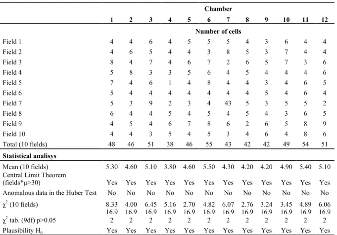
Table 1 - Validity of the sample homogenisation (using 10 fields): the results show the applicability of the Central Limit Theorem, the absence of anomalous data (negative in the Huber Test) and the chi-square values confirm the validity of the homogenisation.

                                                    Chamber 1 2 3 4 5 6 7 8 9 10 11 12 Number of cells Field 1 4 4 6 4 5 5 5 4 3 6 4 4 Field 2 4 6 5 4 4 3 8 5 3 7 4 4 Field 3 8 4 7 4 6 7 2 6 5 7 3 6 Field 4 5 8 3 3 5 6 4 5 4 4 4 6 Field 5 7 4 6 1 4 8 4 4 3 4 6 5 Field 6 5 4 4 4 4 4 4 4 5 4 6 4 Field 7 5 3 9 2 3 4 43 5 3 5 5 2 Field 8 6 4 4 5 4 5 4 5 4 3 6 5 Field 9 4 5 4 6 7 8 6 2 6 5 8 9 Field 10 4 4 3 5 4 5 3 4 6 4 8 6 Total (10 fields) 48 46 51 38 46 55 43 42 42 49 54 51 Statistical analisys Mean (10 fields) 5.30 4.60 5.10 3.80 4.60 5.50 4.30 4.20 4.20 4.90 5.40 5.10 Central Limit Theorem

(fields*µ>30) Yes Yes Yes Yes Yes Yes Yes Yes Yes Yes Yes Yes Anomalous data in the Huber Test No No No No No No No No No No No No χ2 _{(10 fields) 8.33 4.00 6.45 5.16 2.70 4.82 6.07 2.76 3.24 3.45 4.89 6.06} χ2 _{tab. (9df) p>0.05} 16.9₂ 16.9₂ 16.9₂ 16.9₂ 16.9₂ 16.9₂ 16.9₂ 16.9₂ 16.9₂ 16.9₂ 16.9₂ 16.9₂ Plausibility H0 Yes Yes Yes Yes Yes Yes Yes Yes Yes Yes Yes Yes

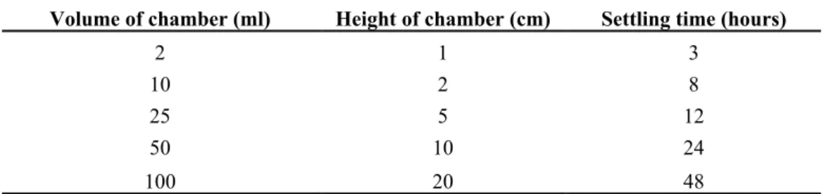
about 8 hours for 10 ml chambers and 48 hours for 50 and 100 ml chambers. Table 3 shows settling times for samples fixed with Lugol solution.

A test performed on formaldehyde-preserved marine phytoplankton counted in 2 ml chambers (about 15 mm high) showed that would have settled by the day after

preparation of the sample, but in 1958 he wrote more explicitly that a settling time of at least 24 hours was needed.

Lund et al. (1958) recommended 18 hours for 100 ml chambers, 3 hours for 10 ml and 1 hour for 1 ml, while Willén (1976) used

Table 2 - Validity of the sub-sample preparation (using 12 chambers): the results show the chi-square values confirm the validity of the sub-sample preparation.

                                                    Chamber 1 2 3 4 5 6 7 8 9 10 11 12 Number of cells Field 1 4 4 6 4 5 5 5 4 3 6 4 4 Field 2 4 6 5 4 4 3 8 5 3 7 4 4 Field 3 8 4 7 4 6 7 2 6 5 7 3 6 Field 4 5 8 3 3 5 6 4 5 4 4 4 6 Field 5 7 4 6 1 4 8 4 4 3 4 6 5 Field 6 5 4 4 4 4 4 4 4 5 4 6 4 Field 7 5 3 9 2 3 4 43 5 3 5 5 2 Field 8 6 4 4 5 4 5 4 5 4 3 6 5 Field 9 4 5 4 6 7 8 6 2 6 5 8 9 Field 10 4 4 3 5 4 5 3 4 6 4 8 6 Total (10 fields) 48 46 51 38 46 55 43 42 42 49 54 51 Statistical analisys

Total cells counted (12 chamber) 565

Average cells/chamber 47.08

χ2 _{(12 chambers) 8.33 4.00 6.45 5.16 2.70 4.82 6.07 2.76 3.24 3.45 4.89 6.06} χ2 _{tab. (11df) p>0.05} 16.9₂ 16.9₂ 16.9₂ 16.9₂ 16.9₂ 16.9₂ 16.9₂ 16.9₂ 16.9₂ 16.9₂ 16.9₂ 16.9₂ Plausibility H0 Yes Yes Yes Yes Yes Yes Yes Yes Yes Yes Yes Yes                          

Volume of chamber (ml) Height of chamber (cm) Settling time (hours)

2 1 3 10 2 8 25 5 12 50 10 24 100 20 48      

Table 3 - Validity of the sub-sample preparation (using 12 chambers): the results show the chi-square values confirm the validity of the sub-sample preparation.

in some cases a period of more than 24 hours was necessary to ensure sedimentation of the algae (Hasle, 1969).

2. Counting subsample

The use of an inverted microscope makes it possible to observe microalgae that have settled on the bottom of the sedimentation chamber. The optical properties of the microscope allow it to discriminate and thus to identify individual organisms. For phytoplankton counting, the inverted microscope should be equipped with a pair of eyepieces (12.5x or 10x), standard objectives (20x, 32x or 40x) and optional objectives (10x, or 100x in the case of immersion, for which immersion oil may be required). One of the objectives should be equipped with an ocular micrometer. In addition there needs to be a space of at least 7 cm between the mount for the laboratory containers and the microscope light, in order to be able to insert a sedimentation chamber of at least 25ml. Filter combinations for autofluorescence (excitation filter 450-490 and barrier filter 515) and epi-fluorescence (excitation filter 340-380 and barrier filter 430) are optional. Also optional but extremely useful is photographic equipment and an image analysis system.

The purpose of microscopic analysis is to determine the structural characteristics of the phytoplankton guild; this analysis is composed of two phases:

a. identification of the microalgal organisms using recognition tests and keys;

b. estimation of cellular density.

In general, when a sedimentation chamber is observed for the first time, a magnification that allows an estimate of both small and large microalgae is used. When the cells are of large dimensions, a lesser magnification (objective 20x) may be used. When recognising microalgal organisms of small dimensions it is necessary to use a high magnification and an immersion objective (100x).

All microalgal organisms observed in the field being explored must be counted. Only living cells need to be counted, discarding empty thecates or cells without organelles such as the nucleus and/or chloroplasts. If a cell or a colony is situated on the boundary between two fields, it should not be counted twice. If it is not possible to identify an organism at the level of genus/species, then classifying on the next taxonomic level up from genus/species is still considered good practice.

To the observer, algae appear to come in a great many shapes and patterns. There are simple unicellular forms with no mechanism for movement, but also highly complex colonial forms with three-dimensional structures. Most algae are of microscopic dimensions but there are also many species that grow in colonies that are large enough to be identified with the naked eye. Fundamentally there are two types of colonial organisation. In some species the colony is composed of an indefinite number of cells, growing by continuous cellular division and reproducing by fragmentation. A second type is composed of a fixed number of cells, very often four or a multiple of four, called a coenobium. Counting strategies

There are three alternative counting strategies when using sedimentation chambers:

a. Strategy 1 - RANDOM FIELD, counting the cells in a number of randomly selected fields;

b. Strategy 2 - TRANSECT, counting the cells in one or more transects;

c. Strategy 3 - BOTTOM, counting the cells in the whole chamber.

A combination of the three counting strategies (figure 1) should be used for each sample, taking account of a few basic considerations: a. Strategy 1 (Cell counts performed on fields).

It requires the operator to randomly select a significant number of fields for each

∑ x is the total number of algal objects counted.

If a precision of 5% in the estimation of the mean number of objects per field is required, then:

x = 1

0.05

!

"

#

$

%

&

'

=

400

That is, 400 objects should be counted. It makes no difference whether 10 fields are counted with 40 objects per field or 80 fields with just 5 objects each

b. Strategy 2 (Cell counts performed on transects)

It entails the identification of the cells along transects of which the length is the same as the diameter of the sedimentation chamber and the width is the same as the diameter of the visual field. The operator should read at least two transects placed perpendicular to each other (also known as the cross method). The number of cells was estimated according to the formula:

C = N !! ! r ! 1000

2! h! v ! n

where:

C = cell abundance, expressed as cells/litre N = total number of cells counted on all transects microalgal species. The number of cells was

estimated according to the formula:

where:

C = cell abundance expressed as cells/litre N = total number of cells counted in all fields A = surface area of the bottom of the sedimentation chamber (in mm2₎

n = number of fields used for cell counts v = volume (in ml) of the sample

a = area of the visual field (in mm2₎

The number of fields or algal objects to count can be set according to the level of precision or detection required, since the precision/ detection limit depends on the number of algal objects/fields counted. The precision (D) of a count can be expressed as either the standard error or as a proportion of the mean or as 95% confidence limit as a proportion of the mean. It has the following formula:

     x n x x n s x mean arithmetic error standard D 1 2 1 1 where:

n is the number of fields counted

x is the mean number of objects per field

C h a m b e r

sedimentation area _Transect

Ocular field

Figure 1. Positioning of the transect and the ocular field.

C = N ! 1000 ! A

n! v ! a

transect for the number of transects counted ; V = is the volume of the sub-sample (in litres).

This detection limit is necessary because it specifies the minimum number of one specific taxon or group of organisms in a sample that will be counted with a certain probability.

Thus, if the quantity of a specific taxon found on the bottom of the sub-sample analysed is below the detection limit, the final result will be that limit and not the value actually counted (see example).

Example

If the detection limit calculated is 120 cells/ litre and if at the end of the reading the following concentrations are obtained: taxon A 4000 cells/litre

taxon B 400 cells/litre taxon C 80 cells/litre

the abundance of taxon C will not be “80 cells/litre” but “< 120 cells/litre”.

Confidence limits for counts with the Poisson distribution

Confidence limits for a total count regardless of the number of fields and objects counted are calculated as follows:

L

=

!

(1!" / 2),#

2

Lower confidence limit (1-α) where:

α = level of significance (set at α = 0.05 – a probability of 95%)

ν = 2x

x = total number of objects counted

_L

2

=

!

2

_{(" / 2),#}

2

Upper confidence limit (1-α) r = radius (in mm) of the sedimentation

chamber

h = height (in mm) of the transect (diameter of the field)

v = volume (in ml) of the sample

n = number of transects used for cell counts c. Strategy 3 (counting a whole chamber) It is performed by traversing backwards and forwards across the chamber, from top to bottom (or vice versa). This strategy is appropriate for detecting rare species or counting large species whose distribution in the chamber may not be random. This type of count requires more time than the other two. The number of cells was estimated according to the formula:

_{C = N ! 1000}

v

where:

C = cell abundance, expressed as cells/litre N = total number of cells counted on all chamber

v = volume (in ml) of the sample Quantitative detection limit

The detection limit (n det) is an important performance characteristic in phytoplankton surveys. For a single taxon (assuming a random distribution), the detection limit may be determined by Poisson statistics in accordance with the formula:

n det =

!ln !

( )

"

ftot

V " fcount

where:

α= is the level of significance (generally 0.05 = probability of 95%);

f _tot = is the total number of microscope fields in the chamber;

f _cont = is the number of fields counted, in the case of count for transect the number of fields is refereed to number of fields in a

of the sub-sample

Once it had been established by direct observation that the algal objects in a sub-sample were distributed randomly with no significant aggregation and no anomalous centripetal or centrifugal distributions, the random distribution of the algal objects in the sub-samples was validated in two step as follows:

- after adequate acclimatisation and homogenisation of the sample, 25 ml were decanted into a sedimentation chamber; - once sedimentation had occurred the absence of anomalies in the distribution was verified visually;

- two algal taxa, Diatoms and Dinoflagellates, were counted along 4 transects passing through the centre of the chamber;

ـ a two-step statistical analysis was applied: 3.1 Step 1 entailed verifying (with where:

α = level of significance (set at α = 0.05 – a probability of 95%)

ν = 2(x+1)

x = total number of objects counted.

As long as a significant part of the chamber is counted, the Poisson series is still applicable. Once the confidence limits have been calculated, they can be expressed in the same unit of measurement as the counts themselves (e.g. cells/litre), multiplying them by the ratio of the total area of the chamber to the area counted (or by the ratio of the number of fields of the chamber to the number of fields counted), and dividing them by the volume of the sub-sample in the chamber.

For every count performed, the upper and lower confidence limits are also calculated. 3. Validation procedures for the preparation

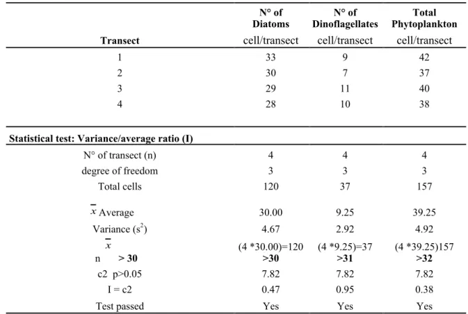
Table 4 - Validation of the preparation of the sub-sample – Step 1 (verification of random distribution).

    Diatoms N° of Dinoflagellates N° of Phytoplankton Total

Transect cell/transect cell/transect cell/transect

1 33 9 42

2 30 7 37

3 29 11 40

4 28 10 38

Statistical test: Variance/average ratio (I)

N° of transect (n) 4 4 4 degree of freedom 3 3 3 Total cells 120 37 157   Average   30.00 9.25 39.25 Variance (s2_{) 4.67 2.92 4.92}   n > 30   (4 *30.00)=120 >30 (4 *9.25)=37 >31 (4 *39.25)157 >32 c2 p>0.05 7.82 7.82 7.82 I = c2 0.47 0.95 0.38

Test passed Yes Yes Yes

x x

reference to the variance/average ratio) that the two taxa were distributed evenly throughout the chamber (verification of random distribution);

The variance/average ratio, which gives a good approximation of the chi-square for n-1 degrees of freedom, is calculated in accordance with the following formula:

I = !

₌

s

(n !1)

x

Where:

x

s2 _{= variance of the number of cells}

The results obtained are summarised in the following table (Table 4).

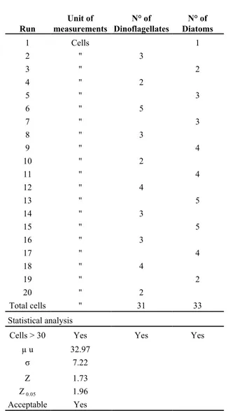
3.2 Step 2 entailed using the Run-test to verify that the order of observation of the taxa was random and thus that subsequent observations of the taxa in question were independent of each other (verification of the independence of subsequent observations). The Run test is used to find out whether two taxa are distributed randomly with respect to each other. If they are distributed randomly, the probability of counting one taxon is independent of the other taxon counted. A run is a sequence of algae of the same taxon counted along a transect:

The Run test can be applied to 2 or more taxa. When a taxon has an abundance of at least 30 objects in the run test count, the average expected quantity of homogeneous sequences (runs) is calculated using the following formula:

µ =

N(N +1) ! n

"

N

N is the total number of algal cells n_i is the number of cells of taxon i.

The average μ has a standard deviation of:

!

(

)

!

!

!

_{( )}

The statistical formula to apply is the following:

_{Z =}

u ! µ

!

0.5

!

                Run test

Run measurements Unit of Dinoflagellates N° of Diatoms N° of

1 Cells 1 2 '' 3 3 '' 2 4 '' 2 5 '' 3 6 '' 5 7 '' 3 8 '' 3 9 '' 4 10 '' 2 11 '' 4 12 '' 4 13 '' 5 14 '' 3 15 '' 5 16 '' 3 17 '' 4 18 '' 4 19 '' 2 20 '' 2 Total cells '' 31 33 Statistical analysis        

Cells > 30 Yes Yes Yes

µ u 32.97 σ 7.22 Z 1.73 Z 0.05 1.96 Acceptable Yes        

Table 5 - Validation of the preparation of the sub-sample – Step 2 (verification of random distribution with respect to each other).

In which u is the number of homogeneous sequences (runs) observed.

The statistic Z can be considered a standardised variable or value Z or normal deviation with Zα(2) as a critical value (Z) of the test (Z _0.05(2) = t _0.05(2), v = 1.96).

The results of the Run test are shown in the following table (Table 5).

References

Directive 2000/60 of the European Parliament and of the Council of 23 October 2000 establishing a framework for community action in the field of water policy. Official Journal L 327/1. Decreto legislativo n°152/2006 della Repubblica Italiana Norme in materia ambientale”.

G.U.88/14/2006.

Hasle GR 1969. An analysis of the phytoplankton of the Pacific southern ocean: abundance, composition, and distribution during the Brategg expedition, 1947-48.

Hvalraedets Skrifter: Scientific Results

of Marine Biological Research 52: 1-168.

Helcom 2001. Manual for Marine Monitoring in the COMBINE Programme of HELCOM. http://www.helcom.fi/Monas/CombineManual2/ CombineHome.htm

Lund JWG, Kipling C, Le Cren ED 1958. The inverted microscope method of estimating algal numbers and the statistical basis of estimations by counting. Hydrobiologia 11: 143-170. UNI EN 15204 “Water quality - Guidance standard

on the enumeration of phytoplankton using inverted microscopy (Utermöhl technique)”. Utermöhl H 1931. Neue Wege in der

quantitativen Erfassung des Planktons

(mit besonderer Berücksichtigung des

Ultraplanktons). Mitteilungen Internationale

Vereiningung fuer Theoretische und

Angewandte Limnologie 5: 567-596.

Utermöhl H 1958. Zur Vervollkommnung der

quantitativen Phytoplankton-Methodik.

Mitteilungen Internationale Vereiningung fuer Theoretische und Angewandte Limnologie 9:

1-38.

Ward TJ, Jacoby CA 1992. A strategy for assessment and riianagement of marine ecosystems: baseline and monitoring studies in Jervis Bay, a temperate Australian embayment.

Marine Pollution Bullettin 25:163-171.

Willén E 1976. A simplified method of

phytoplankton counting. British Phycology