Gravity currents : laboratory experiments and numerical simulations

Roma Tre University

Department of Civil Engineering

Ph.D. in Civil Engineering

XXIV Cycle

Ph.D. Thesis

Gravity currents: laboratory experiments and

numerical simulations

Ph.D. Student: Valentina Lombardi

Tutor: Prof. Giampiero Sciortino

Co-tutors: Dr. Claudia Adduce

Prof. Michele La Rocca

Ph.D. Coordinator: Prof. Leopoldo Franco

Collana delle tesi di Dottorato di Ricerca In Scienze dell’Ingegneria Civile

Università degli Studi Roma Tre Tesi n° 31

Abstract

Gravity currents are buoyancy-driven flows due to a density gradient between two fluids and frequently occur in both natural and industrial flows. In this work two-dimensional and three-dimensional gravity current’s dynamics was investigated by laboratory experiments and numerical simulations. A widely used experimental technique, called lock exchange release was applied to carry out laboratory experiments. In this configuration the tank is divided by a vertical gate into two parts, filled with salty and fresh water, respectively. As soon as the gate is removed, a non-equilibrium condition occurs and the heavier fluid flows under the lighter one, producing the gravity current, whose evolution is recorded by a CCD camera. An image analysis technique, based on the threshold method is then applied in order to measure the space-time evolution of the current’s profile.

Experimental 2D gravity currents were realized in order to study the effect of the density difference between the two fluids and both the roughness and the slope’s angle of the bed on the current’s dynamics. In particular, one of the innovative aspects of this paper is to be focused on gravity currents on upsloping bed, while to the author’s knowledge most of the previous studies deals with currents flowing on downsloping beds. Moreover, regarding 2D configuration, instantaneous velocity measurements were performed by PIV technique (Particle Image Velocimetry). Numerical simulations of 2D gravity currents were performed by a 1D, two-layer, shallow-water model developed by Adduce et al. (2012). The model takes into account the space-time evolution of free-surface and the mixing between the two layers. Entrainment at the interface between the gravity current and the ambient fluid is modeled by a modified Ellison & Turner’s formula (1959). Several tests were run to calibrate an entrainment parameter in order to reproduce gravity currents moving on both smooth flat and upsloping beds.

Experimental 3D gravity currents were carried out in order to test different values of initial density and height of the current and the length of the gate. A single layer, 2D, shallow-water model was used to perform numerical simulations for 3D currents. As for the 1D model, the entrainment is taken into account in the flow’s dynamics.

Experimental results and the comparison between experimental data and numerical prediction for both 2D and 3D configuration are presented, showing that the used models are valid tools to reproduce gravity currents’ dynamics.

Valentina Lombardi

Sommario

Le correnti di gravità sono generate da un gradiente di densità tra due fluidi e rappresentano un fenomeno diffuso in ambito naturale e artificiale. Obiettivo di questo lavoro è l’analisi di correnti di gravità bidimensionali e tridimensionali attraverso esperimenti di laboratorio e simulazioni numeriche. Le correnti di gravità sono state realizzate in laboratorio con una tecnica sperimentale ampiamente diffusa detta “lock exchange release”. Un canale in plexiglass è suddiviso da un setto verticale rimovibile in due volumi distinti, uno riempito con una soluzione acquosa salina e l’altro con acque dolce. Non appena avviene la rimozione del setto, si verifica una condizione di disequilibrio e il fluido più denso scorre al di sotto del fluido ambiente più leggero. L’evoluzione della corrente di gravità così generata è acquisita con una telecamera digitale e una tecnica di analisi d’immagine è stata poi applicata per misurare l’evoluzione spazio-temporale del profilo della corrente.

Le correnti di gravità 2D sono state realizzate allo scopo di studiare l’effetto del gradiente di densità tra i due fluidi, della scabrezza e della pendenza del fondo sulla dinamica della corrente. In particolar modo, il presente lavoro è stato focalizzato sullo studio della dinamica di correnti su fondo acclive, mentre la maggior parte degli studi in letteratura riguarda correnti su fondo declive. Riguardo alla configurazione 2D, sono state realizzate misure istantanee del campo di velocità con la tecnica PIV (Particle Image Velocimetry). Per simulare le correnti 2D è stato utilizzato un modello 1D shallow-water a due strati sviluppato da Adduce et al. (2012). Il modello tiene conto dell’evoluzione spazio-temporale della superficie libera. Il mescolamento all’interfaccia tra i due fluidi è modellato attraverso una forma modificata della formula di Ellison & Turner (1959). Sono state realizzate diverse prove numeriche per calibrare un parametro di mescolamento allo scopo di riprodurre correttamente le correnti di gravità su fondo piano e acclive. Le correnti 3D sono state realizzate allo scopo di esaminare diversi valori di densità iniziale del fluido denso, di altezza iniziale dei due fluidi e di lunghezza del setto. Per le simulazioni numeriche delle correnti 3D è stato utilizzato un modello 2D shallow-water a uno strato sviluppato da La Rocca et al. (2009). Così come il modello 1D, anche il modello 2D tiene conto del mescolamento all’interfaccia tra i due fluidi. Il confronto con le simulazioni numeriche per le correnti di gravità 2D e 3D mostra che i modelli utilizzati sono validi strumenti per la riproduzione della dinamica delle correnti di gravità.

Roma Tre University

Contents

LIST OF FIGURES ... VI LIST OF TABLES ... XIII LIST OF SYMBOLS ... XIV

1. INTRODUCTION ... 1

1.1. THE NATURE OF GRAVITY CURRENTS ... 1

1.2. LOCK EXCHANGE RELEASE... 5

1.3. PREVIOUS STUDIES ... 7 2. 2D GRAVITY CURRENTS ... 15 2.1.LABORATORY EXPERIMENTS ... 15 2.1.1. Experimental set-up ... 15 2.1.2. Experimental parameters ... 16 2.1.3. Experimental results ... 18

2.1.3.1. Flat smooth bed ... 18

2.1.3.2. Rough flat bed ... 22

2.1.3.3. Upsloping smooth bed ... 24

2.2.1D NUMERICAL SIMULATIONS ... 27

2.3.1. Mathematical model ... 27

2.3.2. Numerical method ... 30

2.3.3. Comparison between experimental and numerical results ... 33

2.3.VELOCITY MEASUREMENTS BY PIV ... 41

2.2.1. Flat smooth bed ... 43

2.2.2. Upsloping smooth bed... 48

3. 3D GRAVITY CURRENTS ... 56 3.1.LABORATORY EXPERIMENTS ... 56 3.1.1. Experimental set-up ... 56 3.1.2. Experimental parameters ... 58 3.1.3. Experimental results ... 59 3.2.2D NUMERICAL SIMULATIONS ... 68 3.2.1. Mathematical model ... 68 3.2.2. Numerical method ... 70

3.2.3. Comparison between experimental and numerical results ... 72

4. CONCLUSIONS AND FUTURE AIMS ... 78

REFERENCES ... 81

Valentina Lombardi

List of figures

Figure 1.1: Basic sketch of a gravity current. ... 1 Figure 1.2: Schematic diagram of a gravity current. ... 4 Figure 1.3: Visualization of the area behind the head of a gravity current realized in the Hydraulics Laboratory of University of Rome “Roma Tre”. Instabilities can be observed at the interface between the fluids. ... 4 Figure 1.4: Front of a gravity current of salty water flowing in fresh surrounding water realized in the Hydraulics Laboratory of University of Rome “Roma Tre”. ... 4 Figure 1.5a-b: Sketch of initial conditions for full-depth (a) and partial-depth (b) configuration of lock exchange release experiment. ... 5 Figure 1.6a-f: Images acquired by the camera of a released gravity current: initial configuration (a), flow of the dense fluid (b-f). The time step between the frames is about 1.68 s. ... 6 Figure 2.1: Sketch of the tank used to perform 2D lock release gravity currents. ... 17 Figure 2.2: Picture of the tank used to perform 2D lock release gravity currents. ... 17 Figure 2.3: Measured profiles (white line) overlapping the images captured by the camera for the run 2D_9 at 7, 13, 25 and 38 s after the removal of the gate. ... 17 Figure 2.4a-b: Dimensional and dimensionless plots of front position versus time for the runs 2D_1-2D_5, performed on flat smooth bed with different initial densities. ... 20 Figure 2.5a-c: Measured gravity current’s profiles at three different time steps for the runs 2D_1-2D_5, performed on a flat smooth bed with different initial densities. ... 21 Figure 2.6: Dimensionless log-log plot of front’s position versus time for the runs performed on flat and smooth beds. Dashed line, solid line and dotted line are the theoretical front evolution for the slumping, self-similar and viscous phase, respectively. ... 21

Roma Tre University

Figure 2.7a-h: Dimensional and dimensionless plot of front position versus time for all the runs performed on rough and smooth flat beds; (a-d) Runs 2D_1-2D_6-2D_7-2D_8: ρ011009 Kg/m

3

, ε=0.0, 0.7, 2.2 and 4.5 mm; (b-e) Runs 2D_2-2D_9-2D_10-2D_11: ρ011024 Kg/m 3 , ε=0.0, 0.7, 2.2 and 4.5 mm; (c-f) Runs 2D_3-2D_12-2D_13-2D_14: ρ011039 Kg/m 3 , ε=0.0, 0.7, 2.2 and 4.5 mm; (d-g) Runs 2D_4-2D_15-2D_16-2D_17: ρ011060 Kg/m 3 , ε=0.0, 0.7, 2.2 and 4.5 mm. ... 23 Figure 2.8a-d: Measured gravity current’s profiles at three different time steps for all the runs performed on rough and smooth flat beds; (a) Runs 2D_1-2D_6-2D_7-2D_8: ρ011009 Kg/m 3 , ε=0.0, 0.7, 2.2 and 4.5 mm; (b) Runs 2D_2-2D_9-2D_10-2D_11: ρ011024 Kg/m3, ε=0.0, 0.7, 2.2 and 4.5 mm; (c) Runs 2D_3-2D_12-2D_13-2D_14: ρ011039 Kg/m 3 , ε=0.0, 0.7, 2.2 and 4.5 mm; (d) Runs 2D_4-2D_15-2D_16-2D_17: ρ011060 Kg/m 3 , ε=0.0, 0.7, 2.2 and 4.5 mm. ... 24 Figure 2.9a-c: Measured gravity current’s profiles at three different time steps for all the runs performed on flat and upsloping smooth beds; (a) Runs 2D_3-2D_18-2D_19-2D_20: ρ011039 Kg/m 3 , ϑ=0.0°, 0.90°, 1.11° and 1.39°; (b) Runs 2D_4-2D_21-2D_22-2D_23: ρ011060 Kg/m3, ϑ=0.0°, 1.14°, 1.39° and 1.52°; (c) Runs 2D_5-2D_24-2D_25-2D_26: ρ011090 Kg/m 3 , ϑ=0.0°, 1.39°, 1.45° and 1.8°. ... 25 Figure 2.10a-f: Dimensional and dimensionless plots of front position versus time for all the runs performed on flat and upsloping smooth beds; (a-d) Runs 2D_3-2D_18-2D_19-2D_20: ρ011039 Kg/m

3

, ϑ=0.0°, 0.90°, 1.11° and 1.39°; (b-e) Runs 2D_4-2D_21-2D_22-2D_23: ρ011060 Kg/m 3 , ϑ=0.0°, 1.14°, 1.39° and 1.52°; (c-f) Runs 2D_5-2D_24-2D_25-2D_26: ρ011090 Kg/m 3 , ϑ=0.0°, 1.39°, 1.45° and 1.8°. ... 26 Figure 2.11: Frame of reference used in the mathematical model. ... 27 Figure 2.12: Sketch of grid points involved in a predictor-corrector step. .... 32 Figure 2.13a-d: Comparison of numerical gravity current’s profiles for the run 2D_4 moving on flat and smooth bed and the images acquired by the camera at four different time steps: miscible fluid, k=0.6 (solid yellow line) and immiscible fluid, k=0 (red dashed line). ... 36

Valentina Lombardi

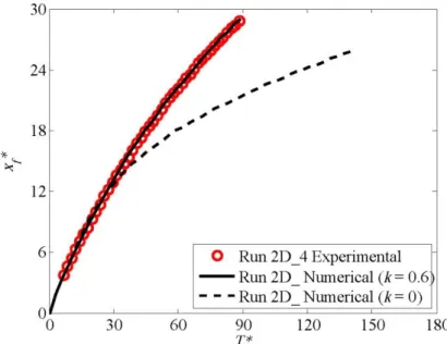
Figure 2.14: Front position versus time for the run 2D_4 moving on flat and smooth bed: measurements (red circles), numerical simulation with k=0.6 (black solid line) and numerical simulation with k=0.0 (black dashed line). ... 36 Figure 2.15a-d: Comparison of numerical gravity current’s profiles for the

run 2D_21 moving on smooth and upsloping bed and the images acquired by the camera at four different time steps: miscible fluid, k=0.9 (solid yellow line) and immiscible fluid, k=0 (red dotted line). ... 37 Figure 2.16: Front position versus time for the run 2D_21 moving on smooth and upsloping bed: measurements (red circles), numerical simulation with k=0.9 (black solid line) and numerical simulation with k=0.0 (black dotted line). ... 37 Figure 2.17a-d: Experimental and numerical front position versus time for all the runs performed with ρ011039 Kg/m3 on flat and upsloping smooth beds; (a) Run 2D_3: ϑ=0.00°; (b) Run 2D_18: ϑ=0.90°; (c) Run 2D_19: ϑ=1.11°; (d) Run 2D_20: ϑ=1.39°. ... 38 Figure 2.18a-d: Experimental and numerical front position versus time for all the runs performed with ρ011060 Kg/m3 on flat and upsloping smooth beds; (a) Run 2D_4: ϑ=0.00°; (b) Run 2D_21: ϑ=1.14°; (c) Run 2D_22: ϑ=1.39°; (d) Run 2D_23: ϑ=1.52°. ... 39 Figure 2.19a-d: Experimental and numerical front position versus time for all

the runs performed with ρ011090 Kg/m

3

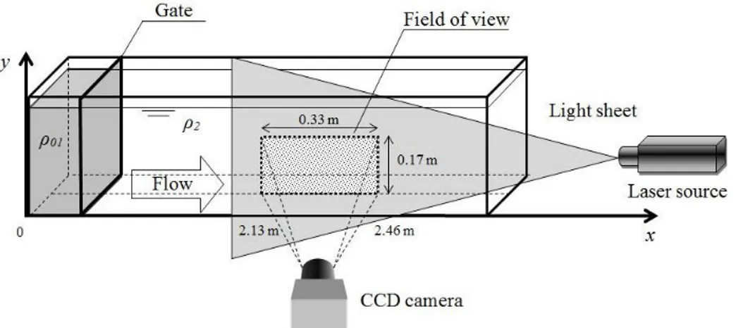
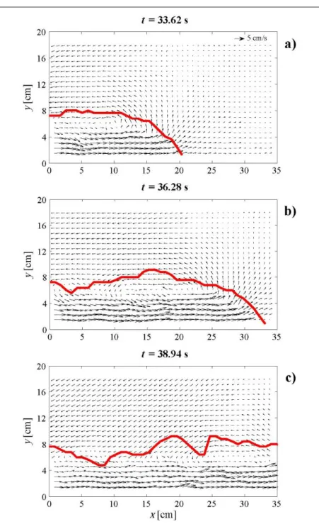
on flat and upsloping smooth beds; (a) Run 2D_5: ϑ=0.00°; (b) Run 2D_24: ϑ=1.39°; (c) Run 2D_25: ϑ=1.45°; (d) Run 2D_26: ϑ=1.80°. ... 40 Figure 2.20: Sketch of a general PIV system showing the main components: tank with transparent wall filled with fluid seeded with tracer particles, laser source producing laser sheet, camera acquiring images in the area of interest. ... 42 Figure 2.21: Sketch of the PIV system used for velocity measurements showing the field of view analyzed for the run PIV1. ... 43 Figure 2.22a-c: Vector maps of the gravity currents at three different time steps. The red line is the interface between the two fluids, identified as the height of a colored release current performed with the same experimental parameters. Threshold method was applied to measure the profile of the current acquired by a CCD camera. ... 45

Roma Tre University

Figure 2.23a-b: Contour plots of the x-velocity component, u, (a) and vorticity ω (b) at six time steps for the run PIV1. ... 46 Figure 2.24a-c: x-velocity component measured along x-axis for three different heights y1, y2 and y3 at t=33.62 s for the run PIV1. The dashed black line corresponds to the x-velocity component equals to zero. ... 47 Figure 2.25a-c: Vertical profiles of the x-velocity component measured at three different positions x1, x2 and x3 at for t=33.62 s for the run PIV1. The dashed black line corresponds to the x-velocity component equals to zero, while with the red dashed line is showed the height of the gravity current for each position on the x-axis. ... 47 Figure 2.26: Comparison for the run PIV1 between x-velocity component

measured by PIV (red circles) and x-velocity component predicted by numerical simulation by 1D numerical model (green line) at t=36.28 s. Velocity values measured by PIV are averaged along the y-axis. The dashed black line corresponds to u equal to zero. ... 48 Figure 2.27: Sketch of the PIV system used for velocity measurements

showing the field of view analyzed with the run PIV2. ... 49 Figure 2.28a-c: Vector maps of the gravity currents at three different time steps. The red line is the interface between the two fluids, identified as the height of a colored release current performed with the same experimental parameters. Threshold method was applied to measure the profile of the current acquired by a CCD camera. ... 50 Figure 2.29a-b: Contour plots of the x-velocity component, u, (a) and vorticity ω (b) at six time steps for the run PIV2. ... 51 Figure 2.30: Vector maps of the gravity currents at t=34.33 s. Velocity field is shown for a detailed area of the field of view, 20 cm long and 14 cm high. The red line is the interface between the two fluids. ... 52 Figure 2.31a-b: Contour plots of the x-velocity component, u, (a) and vorticity ω (b) of the gravity currents at t=34.33 s for a detailed area of the field of view, 20 cm long and 14 cm high. ... 53 Figure 2.32a-c: x-velocity component measured along x-axis for three different heights y1, y2 and y3 at t=34.33 s for the run PIV2. The

Valentina Lombardi

dashed black line corresponds to the x-velocity component equals to zero. ... 54 Figure 2.33a-c: Vertical profiles of the x-velocity component measured at three different positions x1, x2 and x3 at for t=34.33 s for the run PIV2. The dashed black line corresponds to the x-velocity component equals to zero, while with the red dashed line is showed the height of the gravity current for each position on the x-axis. ... 54 Figure 2.34: Comparison for the run PIV2 between x-velocity component

measured by PIV (red circles) and x-velocity component predicted by numerical simulation by 1D numerical model (green line) at t=8.66 s. Velocity values measured by PIV are averaged along the y-axis. The dashed line corresponds to u equal to zero. ... 55 Figure 2.35: Comparison between x-velocity component measured by PIV (red circles) and x-velocity component predicted by numerical simulation by 1D numerical model (green line) at t=34.66 s. Velocity values measured by PIV are averaged along the y-axis. The dashed line corresponds to u equal to zero. ... 55 Figure 3.1a-c: Experimental apparatus used to perform the 3D lock-exchange experiments: (a) sketch of the top view; (b) sketch of the side view; (c) picture of the tank. ... 57 Figure 3.2a-d: Evolution on the x-y plane of the run 3D_1: measured profiles overlapped to the images corresponding to 6 s (a), 12 s (b), 18 s (c) and 24 s (d) after the release of the lock fluid. ... 58 Figure 3.3a-f: Dimensional and dimensionless plot of front positions versus

time for the runs with ρ011010 Kg/m

3

; (a-d) Runs 3D_1-3D_2-3D_3: h0=0.15 m, d=0.135, 0.35, 0.67 m; (b-e) Runs 3D_4-3D_5-3D_6: h0=0.10 m, d=0.135, 0.35, 0.67 m; (c-f) Runs 3D_7-3D_8-3D_9: h0=0.05 m, d = 0.135, 0.35, 0.67 m. ... 61 Figure 3.4a-f: Dimensional and dimensionless plot of front positions versus

time for the runs with ρ011030 Kg/m

3 ; (a-d) Runs 3D_10-3D_11-3D_12: h0=0.15 m, d=0.135, 0.35, 0.67 m; (b-e) Runs 3D_13-3D_14-3D_15: h0=0.10 m, d=0.135, 0.35, 0.67 m; (c-f) Runs 3D_16-3D_17-3D_18: h0=0.05 m, d=0.135, 0.35, 0.67 m. ... 62 Figure 3.5a-f: Dimensional and dimensionless plot of front positions versus time for the runs with h0=0.15 m; (a-d) Runs 3D_1-3D_10:

Roma Tre University d=0.135 m, ρ011010, 1030 Kg/m 3 ; (b-e) Runs 3D_2-3D_11: d=0.35 m, ρ011010, 1030 Kg/m 3 ; (c-f) Runs 3D_3-3D_12: d=0.67 m, ρ011010, 1030 Kg/m 3 . ... 63 Figure 3.6a-f: Dimensional and dimensionless plot of front positions versus time for the runs h0=0.10 m; (a-d) Runs 3D_4-3D_13: d=0.135 m, ρ011010, 1030 Kg/m 3 ; (b-e) Runs 3D_5-3D_14: d=0.35 m, ρ011010, 1030 Kg/m 3 ; (c-f) Runs 3D_6-3D_15: d=0.67 m, ρ011010, 1030 Kg/m 3 . ... 64 Figure 3.7a-f: Dimensional and dimensionless plot of front positions versus time for the runs with h0=0.05 m; (a-d) Runs 3D_7-3D_16:

d=0.135 m, ρ011010, 1030 Kg/m 3 ; (b-e) Runs 3D_8-3D_17: d=0.35 m, ρ011010, 1030 Kg/m3; (c-f) Runs 3D_9-3D_18: d=0.67 m, ρ011010, 1030 Kg/m 3 . ... 65 Figure 3.8a-f: Dimensional and dimensionless plot of front positions versus

time for the runs with ρ011010 Kg/m

3

; (a-d) Runs 3D_1-3D_4-3D_7: d=0.135 m, h0=0.15, 0.10, 0.05 m; (b-e) Runs 3D_2-3D_5-3D_8: d=0.35 m, h0=0.15,0.10, 0.05 m; (c-f) Runs 3D_3-3D_6-3D_9: d=0.67 m, h0=0.15,0.10, 0.05 m. ... 66 Figure 3.9a-f: Dimensional and dimensionless plot of front positions versus

time for the runs with ρ011030 Kg/m

3

; (a-d) Runs 3D_10-3D_13-3D_16: d=0.135 m, h0=0.15,0.10, 0.05 m; (b-e) Runs 3D_11-3D_14-3D_17: d=0.35 m, h0=0.15,0.10, 0.05 m; (c-f) Runs 3D_12-3D_15-3D_18: d=0.67 m, h0=0.15,0.10, 0.05 m. 67 Figure 3.10: Sketch of the frame of reference used for the 2D mathematical model. ... 69 Figure 3.11a-c: Dimensionless plot of experimental and numerical front positions versus time for the runs performed with ρ011010 Kg/m3. (a) Runs 3D_1-3D_2-3D_3 performed with h0=0.15 m and d=0.135, 0.35, 0.67 m, respectively; (b) Runs 3D_4-3D_5-3D_6 performed with h0=0.10 m and d=0.135, 0.35, 0. 67 m, respectively; (c) Runs 3D_7-3D_8-3D_9 performed with h0=0.05 m and d=0.135, 0.35, 0.67 m, respectively. The front position is detected along the centerline of the tank. ... 74 Figure 3.12a-c: Dimensionless plot of experimental and numerical front positions versus time for the runs performed with ρ011030 Kg/m3. (a) Runs 3D_10-3D_11-3D_12 performed with h0=0.15 m and d=0.135, 0.35, 0.67 m, respectively; (b) Runs 3D_13-3D_14-3D_15 performed with h0=0.10 m and d=0.135, 0.35,

Valentina Lombardi

0.67 m, respectively; (c) Runs 3D_16-3D_17-3D_18 performed with h0=0.05 m and d=0.135, 0.35, 0.67 m, respectively. The front position is detected along the centerline of the tank. ... 75 Figure 3.13a-i: Comparison between experimental and numerical wave front

for the runs performed with ρ011010 Kg/m

3

. (a) Run 3D_1: h0=0.15 m and d=0.135 m; (b) Run 3D_2: h0=0.15 m and d=0.35 m; (c) Run 3D_3: h0=0.15 m and d=0.67 m; (d) Run 3D_4:

h0=0.10 m and d=0.135 m; (e) Run 3D_5: h0=0.10 m and d=0.35 m; (f) Run 3D_6: h0=0.10 m and d=0.67 m; (g) Run 3D_7:

h0=0.05 m and d=0.135 m; (h) Run 3D_8: h0=0.05 m and d=0.35 m; (i) Run 3D_9: h0=0.05 m and d=0.67 m. ... 76 Figure 3.14a-i: Comparison between experimental and numerical wave front

for the runs performed with ρ011030 Kg/m

3

. (a) Run 3D_10: h0=0.15 m and d=0.135 m; (b) Run 3D_11: h0=0.15 m and

d=0.35 m; (c) Run 3D_12: h0=0.15 m and d=0.67 m; (d) Run 3D_13: h0=0.10 m and d=0.135 m; (e) Run 3D_14: h0=0.10 m and d=0.35 m; (f) Run 3D_15: h0=0.10 m and d=0.67 m; (g) Run 3D_16: h0=0.05 m and d=0.135 m; (h) Run 3D_17: h0=0.05 m and d=0.35 m; (i) Run 3D_18: h0=0.05 m and d= .67 m. ... 77

Roma Tre University

List of tables

Table 1: Experimental parameters used to perform 2D gravity currents. ... 18 Table 2 Lengths of slumping phase ls, self-similar phase lss and viscous phase

lvis for all the runs performed on flat and smooth beds. ... 20 Table 3: Experimental parameters and calibration values of k for all the runs performed on smooth flat and upsloping beds. ... 33 Table 4: Experimental parameters and mean error Exf computed for each run on the basis of Equation (41) for all the 2D released currents performed on smooth flat and upsloping beds. ... 35 Table 5: Experimental parameters used to perform 3D gravity currents. ... 59 Table 6: Experimental parameters and mean error Exf computed for each run on the basis of Equation (60) for all the 3D released currents. ... 73

Valentina Lombardi

List of symbols

b Width of the tank – 2D experiments

B Width of the tank – 3D experiments

C Depth averaged concentration – 2D model

d Length of removable gate – 3D experiments

g Gravity acceleration

g' Reduced gravity acceleration

h* Non-constant height of current’s shape h0 Initial height of the lock fluid

h1; h2 Height of dense and ambient fluid – 1D model

H Total height of the two fluids

k Dimensionless entrainment parameter – 1D model l* Transition point between self-similar and viscous phase ls;lss;lvis Length of slumping, self-similar and viscous phase

L Half length of the tank – 3D experiments u x-velocity component

U Depth averaged x-component velocity – 2D model

Uf Front’s velocity

Um Velocity modulus – 2D model

Roma Tre University

V1; V2 Velocity of dense and ambient fluid – 1D model

Ve Entrainment velocity – 1D model

Txz|z=0; Tyz|z=0 Bottom stresses – 3D model

x0 Gate position – 2D experiments

xf Front’s position

α Entrainment coefficient – 2D model

 Bed’s roughness

ϑ Slope’s angle of the tank

λ1; λ2 Friction factor for lower and upper layer – 1D model

λint Friction factor at the interface – 1D model

λ∞ Friction factor for turbulent rough flows

μ Dynamic viscosity

ν Kinematic viscosity

ρ01 Initial density of the heavier lock fluid

ρ1; ρ2 Density of dense and ambient fluid

ρp Density of reflective particles

ρs Density of sediments

τ1b ; τ2b Bottom stresses – 1D model

τ12 Stress term at the interface – 1D model

1. Introduction

1.1. The nature of gravity currents

Gravity currents, also called density or buoyancy currents, are flows generated by a density gradient between two fluids and occur in both natural and industrial flows. A large variety of examples of gravity currents can be found in Simpson, 1997. The basic sketch of a typical gravity current configuration is shown in Figure 1.1. The gravity current with density ρ1 propagates into the ambient fluid with a different density ρ2. If ρ1>ρ2 the more dense (heavy) fluid flows below the upper layer, generating a bottom gravity current, while if ρ2>ρ1 a top current of less dense (light) fluid occurs. Gravity currents can also occur as intrusions of mixed fluid in a sharply or linearly stratified ambient (Ungarish, 2009). The former case of a bottom current is the object of this work. In this configuration (i.e. ρ1>ρ2), the current with higher density ρ1 and non-constant depth h* moves

forward with front’s velocity Uf into the surrounding fluid with lower density ρ2. The total depth of the two fluids is H. Behind the head of the current mixing and instabilities are concentrated. Underneath this area sedimentation and resuspension of particles can occur, if sediments are carried by the current.

Figure 1.1: Basic sketch of a gravity current.

Gravity currents frequently develop along the longitudinal direction, so that the ratio of the vertical scale of the current to the horizontal length scale is small enough to allow the application of the shallow-water theory.

In the gravity current’s shape a head and a tail can be distinguished. The head is located at the leading edge, and it is almost twice as high as the following flow (Simpson, 1982), frequently called tail of the current. In the frontal zone of the current (i.e. the head) a nose rising above the following flow can usually be observed (Simpson, 1997).

In a typical gravity current configuration, hydrostatic balance can be assumed in the z-direction. Regarding the horizontal direction the density difference causes a pressure difference in the x-direction, which is then balanced by the velocity field with a main horizontal component Uf (Ungarish, 2009). Therefore the gravity current is driven by the gravity force and the gravity effect related to the density gradient is called reduced gravity g' and is defined in this work as:

2 2 1 2 ' ρ ρ ρ g ρ ρ g g     (1)

where g is the gravity acceleration. The advantage of using g' is that in its own definition a large range of the ratio ρ1/ρ2 are included.

It’s possible to distinguish Boussinesq and non-Boussinesq gravity currents. The former are characterized by a relatively small difference between the densities of the two fluids involved in the flow. Hence in this case ρ1ρ2, or ρ1/ρ21. Non- Boussinesq gravity currents are the ones for which the above condition is not verified.

Moreover gravity currents can be classified also as compositional or particle-driven gravity currents. In the case of compositional gravity currents the driving force is represented by dissolved solute like salt in the sea or difference of temperature, while for particle-driven gravity currents the driving force is represented by the suspension of sediments. A combination of the two types can also occur. Examples of compositional gravity currents are the sea breeze winds and submarine currents; the former are driven by a temperature gradient, while the latter are driven by a difference in salinity. Particle driven gravity currents are also common phenomena in natural environment, for example sandstorms and avalanches. The currents studied in the present work are all of Boussinesq type and the density difference between ρ1 and ρ2 is due to a difference in concentration of salt dissolved in the fluids (i.e. compositional gravity currents). Front speed Uf can be roughly estimated by applying Bernoulli’ law to a simplified scheme shown in Figure 1.2. Assuming a frame of reference moving with the front, the fluid in the current is at rest and the surrounding fluid moves toward the current’s front with propagation velocity -Uf. Assuming a hydrostatic pressure distribution, equating the values of potential and kinetic energy between points O and N, the following relation can be obtained:





h g gh ρ ρ ρ Uf ' 1 2 1   (3)

Although Equation (3) is estimated on the basis of a very simple energy balance assuming some simplifications, it represents a starting value for the speed of propagation of the typical gravity current.

An important dimensionless parameter for a Boussinesq gravity current is the Froude number Fr, defined as the ratio of the current speed U and the long wave speed

g'

h

Equation (4) shows that Froude number is a dimensionless representation of the speed of the current.

Another important dimensionless parameter is the Reynolds number Re, defined as:

ν Uh

Re (5)

where  is the kinematic viscosity. Equation (5) shows that Reynolds number measures the importance of viscous dissipation on the current. Simpson (1997) suggested that for values of Reynolds numbers greater than 1000 viscous effects are unimportant.

The two main types of instabilities involved in gravity current’s dynamics are Kelvin-Helmotz billows and the lobes-and-clefts structure. Kelvin-Helmotz billows roll up in the region of velocity shear above the front of the current, contributing to the mixing processes behind the current’s head. The complex lobes-and-clefts shifting is due to the gravitational instabilities of the less dense ambient fluid which is overrun by the nose of the gravity current (Simpson, 1997).

Figure 1.3 and Figure 1.4 show two images referred to laboratory experiments performed in the Hydraulics Laboratory of University of Rome “Roma Tre”. The currents were realized by a lock exchange release, a widely used experimental technique that will be fully explained in section 1.2. In Figure 1.3 a visualization of the area behind the head of a gravity current is shown. Vortexes

are visible at the interface between the two fluids due to the velocity shear between the two layers with different densities.

The frontal region of a typical gravity current can be observed in Figure 1.4. The currents in Figure 1.3 and in Figure 1.4 were made visible by adding some white colorant to the dense fluid.

Figure 1.2: Schematic diagram of a gravity current.

Figure 1.3: Visualization of the area behind the head of a gravity current realized in the

Hydraulics Laboratory of University of Rome “Roma Tre”. Instabilities can be observed at the interface between the fluids.

Figure 1.4: Front of a gravity current of salty water flowing in fresh surrounding water

1.2. Lock exchange release

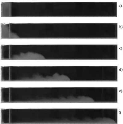
An experimental technique widely used to produce laboratory gravity currents is the lock-exchange release. In this configuration a tank is divided in two portions separated by a vertical sliding gate, one filled with lighter fluid (e.g. fresh water), and the other filled with the heavier one (e.g. salty water). It’s possible to distinguish two different initial configurations: a full depth (Figure 1.5a) if the initial heights of the two fluids are the same and partial-depth (Figure 1.5b) if the initial height of the dense fluid is only a fraction of the whole height. The present work deals with full-depth experiments. The experiment begins when the gate is suddenly removed and a non-equilibrium condition occurs between the two fluids. Hence the heavier fluid flows under the lighter one, producing the gravity current. The experiment stops when the current’s front reaches the right end wall of the tank. Figure 1.6a-f show the images acquired by a CCD camera of a gravity current produced by a full-depth lock exchange experiment in a Perspex tank in the Hydraulics Laboratory of University of Rome “Roma Tre”. The time step between the images is about 1.68 s. In Figure 1.6a the initial configuration is shown, while in Figure 1.6b-f the resulting flow from the release of the dense fluid can be observed: the dense gravity current moves to the right part of the tank along the bottom boundary, while the buoyant current (i.e. ambient fluid) flows to left along the upper boundary.

Figure 1.5a-b: Sketch of initial conditions for full-depth (a) and partial-depth (b)

configuration of lock exchange release experiment.

Huppert & Simpson (1980) and Rottman & Simpson (1983) investigated gravity currents performing lock exchange experiments in a channel of rectangular

cross-section and showed that three phases can be distinguished in the dynamics of a gravity current produced by an instantaneous release. The first phase, called slumping phase, is characterized by a constant speed and a linear variation of the front position with time. During the second phase, called self-similar phase, the front’s speed depends on time by a power law as t-1/3

and the front position varies with t2/3 (Rottman & Simpson, 1983). The transition between the first and the second phase occurs when a bore, caused by the reflection of the lighter fluid to the left wall of the tank, reaches the current’s front, which is slower than the bore. Rottman & Simpson (1983) found that the first phase stops at a distance from the left wall, ls, given by:

0

10 x l

x_f  _s   (6)

where xf is the front position and x0 is a length scale defined as the distance between the gate and the left vertical wall of the tank.

Figure 1.6a-f: Images acquired by the camera of a released gravity current: initial

configuration (a), flow of the dense fluid (b-f). The time step between the frames is about 1.68 s.

If viscous and inertial forces become comparable, a third viscous phase occurs and the current’s speed decreases with a law as t-4/5

, while the front position increases with t1/5 (Huppert, 1982). Huppert (1982) also found that the transition between the self-similar phase and the viscous phase is reached when xfl* with

l* defined as: 7 1 2 5 0 5 0 0 * '        ν x h g l (7)

where h0 is the initial height of the heavier fluid, ν is the kinematic viscosity of the dense fluid and g0' is the initial reduced gravity, defined as:

2 2 01 0 ' ρ ρ ρ g g   (8)

in which ρ01 is the initial density of the gravity current and ρ2 is the density of the ambient fluid.

1.3. Previous studies

Many studies investigated gravity currents by both laboratory experiments and numerical simulations.

The first quantitative study of gravity currents was an essay, published by von Kármán in 1940, proposing a perfect-fluid model for steadily propagating gravity currents. The motivation of such a study was an enquiry by the American military before the War World II concerning the evaluation of what wind conditions would allow to poisonous gas to move forward and reach the enemy avoiding the backwards flow towards the troops who released the substance (Huppert, 2006). He considered a frame of reference moving with the dense fluid (of density ρ1), which is therefore assumed to be at rest, while the ambient fluid (of density ρ2) of infinite depth appears to be in stationary motion above the interface between the two layers, with propagation velocity c1. On the basis of Bernoulli’s theorem von Kármán found that the angle formed between the interface and the bottom at the stagnation point is 60°. Moreover, by applying the Bernoulli’s theorem between the stagnation point and several points at the interface where this is supposed to become horizontal, he obtained a relation for

the velocity of the flow along the interface. The dimensionless speed found by von Kármán is given by:

H g c Fr_H ' 1  ₍₉₎

where H is the asymptotic height of the interface. The Froude number was evaluated by von Kármán to be 2. For gravity flows propagating into a very deep ambient at high Reynolds number, the condition proposed by von Kármán has been generally applied at the nose of the current.

Benjamin (1968) argued that von Kármán (1940) used incorrectly the Bernoulli’s theorem by applying it along the interface, where dissipation takes place. By using a momentum integral, Benjamin obtained the same result as von Kármán.

A simple theory by Prandt (1952) concerns the transient phase following the release of dense fluid in a deep surrounding fluid with lower density. Neglecting hydrostatic forces and applying the hypothesis that the roll formed at the rear of the head of the current does not fall backward, Prandt (1952) obtained the ratio of the propagation velocity to the flow velocity by the evaluation of the dynamic pressures against the front. Prandt’s theory can only be applied to the transient phase, during which the gate between the two fluids is partially opened. In fact, as soon as the gate is removed, the roll formed at the rear of the head of the currents falls behind and entrained with the lower layer, developing a turbulent motion at the front. After this stage of development, a state of stationary propagation takes place, in which turbulent motion is confined to the head of the current and the ratio of the propagation velocity to the flow velocity must be 1 (Benjamin, 1968).

As previously touched on, Benjamin provides an alternative argument leading to the same results of von Kármán, by the use of a momentum integral, or flow force, as himself called it in Benjamin (1968). Benjamin develops its theory for a cavity empty or filled with air, whose weight can be neglected. Shin et al. (2004) proposed Benjamin’s theory on the basis of an idealized two-dimensional gravity current of density ρ2 which flows with constant velocity U into a surrounding fluid with density ρ1. The frame of reference moves with the front. The total depth of the two layers is H, while the depth of the current, where the interface becomes flat, is h. The velocity of the ambient fluid is supposed to be constant and it is denoted as u1. The control volume is delimited by two horizontal boundaries and two vertical planes, one downstream and one upstream. As no external forces are involved in the system, the net flux of horizontal momentum into the considered control volume is zero. By the use of continuity equation and conservation of the horizontal component of the

momentum flux between the vertical sections, taking into account the hydrostatic pressure distribution, the following relation can be obtained:

) ( 1 2 h f γ γ gH U   (10)

where γ is the density ratio ρ1/ ρ2 and f(h) is given by:











The Froude number FH is then defined as:





Benjamin (1968) showed that if dissipation can be neglected, Bernoulli’s theorem can be applied along another streamline, which can be the top boundary or the interface between the two fluids and the following definition can be obtained:



 



Equating relations (10) and (13), two solutions for h/H are provided:

2 1 0   H h H h (14)

The second solution says that the current must occupy half the distance between the horizontal plates if the flow as to be steady and without energy dissipation. Considering a Bossinesq current, the density ratio γ=1, hence the Froude number FH is defined as:





Benjamin (1968) reached the same results of von Kármán, for the case of a gravity current moving into an infinitively deep ambient fluid. Hence for the case of H, h/H=0 and the Froude number in terms of depth of the current h is found to be 2, as von Kármán suggested.

Rottman & Simpson (1983) proposed a shallow-water model considering the current as a two-dimensional two-layer flow bounded at the top and at the bottom by horizontal planes. They considered the partial-depth lock release (Figure 1.5b), involving two inviscid, incompressible fluids with slightly different densities and assumed mixing negligible. They imposed the following front condition:







where Uf is the front’s speed, hf is the depth at the front and β is a dimensionless constant.

More recently, Shin et al. (2004) considered the case of a partial-depth lock exchange experiments. They developed an hydraulic model for unsteady and irrotational flow, in which, for high Reynolds number, the energy dissipation is a weak component. In contrast with Benjamin’s theory they included in the control volume both the current’s front and the wave depression. The fluid is assumed to be inviscid and immiscible, and the pressure distribution is assumed to hydrostatic. Moreover they supposed an horizontal surface between the depression wave and the current’s front.

By the use of continuity equation and horizontal momentum conservation, and applying time-dependent Bernoulli’s theorem and choosing a suitable velocity potential, Shin et al. (2004) found the following definition for the speed of the current:



 













where D is the lock depth, h is the current’s depth and H is the total depth of the two fluids. As for the Benjamin’s theory, in order to specify h, a further

condition is needed. Therefore Shin et al. (2004) assumed an energy-conserving flow, in order to equate energy gain and energy loss in the control volume and obtain a further relation for the current speed:

















Comparing Equation (17) and Equation (18) the only non-trivial solution is given by:

2 D

h (19)

This results shows that an energy-conserving current produced by a partial-depth release has an height which is half of the initial height of the lock. Such result is consistent with Benjamin’s result (Equation 14) for a full-depth release. Using Equation (19) the speed of the current for a Boussinesq gravity current (i.e. 1) is:





For a full-depth release Equation (20) leads to the Benjamin’s results FH=1/2, while for the case of a partial-depth release the presented theory differs from Benjamin’s one.

Marino et al. (2005), on the basis of their experimental results showed that during the slumping phase (i.e. constant-speed phase) the Froude number can be defined in terms of lock depth, while during the second similar phase, which is no more influenced by the initial conditions, the Froude number is better defined on the basis of the maximum height of the current’s head, which corresponds to the height at the rear of the head. They also found that Froude number defined in such way is dependent on the Reynolds number over the range 400-4500. More recently, La Rocca et al. (2008) studied the dynamics of three-dimensional gravity currents moving on smooth and rough beds by full-depth lock exchange experiments and numerical simulations, using a 2D shallow water model together with the single layer approximation. They investigated gravity current’s dynamics keeping constant the width of the sliding gate, the initial density of the lighter fluid and testing different values of initial density of the dense fluid,

initial height of the two fluids and the bed’s roughness. They observed two different phases in three-dimensional gravity current’s evolution: the front’s velocity increases during the first phase and decreases during the second phase. La Rocca et al. (2008) suggested that these phases cannot be interpreted as slumping and self-similar phases, typical of two-dimensional and axisymmetric gravity currents. In fact as explained in section 1.2, the slumping phase is related to the backward flow of the upper layer of lighter fluid and to its reflection on the end-wall of the tank. As soon as the reflected wave overtakes the current’s front, the gravity current starts to decelerate and the second self-similar phase starts. The geometrical configuration used in La Rocca et al. (2008) consists in a rectangular tank divided into two square section reservoirs of equal dimension by a vertical sliding gate, whose length is only a fraction of the total width of the tank. Therefore the backward-forward flow of the depression wave is influenced by the length of the gate, which chokes the flow and causes a configuration of permanent motion through the gate’s opening; such a behavior does not allow the overtaking of the front by the depression wave and consequently the self-similar phase never starts. They also found that as the bed’s roughness increases, the front’s velocity during the second phase decreases. They observed a fairly good agreement in the velocity and front position between experimental and numerical results, although they observed a systematic discrepancy between them during the first instants of motion, which is attributed by the authors to the neglecting of the entrainment term in the mathematical model. Adduce et al. (2012) performed two-dimensional full-depth lock exchange experiments on a flat bed and compared experimental results with numerical simulations obtained by a two-layer, 1D shallow water model for miscible fluids. They carried out several laboratory experiments varying the lock position, the initial height of the two fluids and the initial density of the dense gravity current. Unlike several previous studies, Adduce et al. (2012) removed the rigid lid approximation, accounting for the free surface effects, and took into account also the entrainment between the two fluids. The latter is model by a modified Ellison & Turner’s formula. The modeling of the mixing between the two fluids is a novelty, as shallow water models rarely presents this features. They proposed a comparison between numerical prediction with and without taking into account the entrainment, showing a better agreement with experimental results for the simulation performed for miscible fluids. Moreover, they showed the free surface effect, by comparing the numerical results obtained with the proposed model, accounting for both the free-surface oscillation and the mixing between the two layers, and single layer models with a rigid lid assumption. They compared experimental front’s velocity, measured during the first slumping phase, with the one predicted by their model and previous expressions found in literature and they observed that the best agreement with experimental results is provided by using their own model. A recent paper by La Rocca et al. (2012) investigated the dynamics of a two-layer liquid, made of two immiscible

shallow-layers of different density within the framework of the Lattice Boltzmann Method (LBM). Results obtained from the LBM are compared with numerical results obtained with a two-layer shallow-water model, with experimental results and other numerical results published in literature. They observed that the prediction obtained by using the LBM and the one obtained with the shallow-water model can be considered almost equivalent and agree well with experimental results during the initial phase of the flow, when viscous forces are not involved in the evolution of the current. They also showed that the LBM is a valid tool to simulate gravity currents moving on beds with different slopes.

Several authors studied gravity current by the use of high resolution numerical models as LES (Ooi et al., 2007) or DNS (Härtel et al., 2000a-b; Cantero et al. 2006; Cantero et al. 2007). Such models provide a very detailed description of gravity current’s dynamics, producing reliable results. However they are very complex and require high computational resources.

Some works were focused on measuring the velocity field during the slumping phase. Thomas & al. (2003) defined the two-dimensional structure of the head of inertial gravity currents during the slumping phase by digital Particle Tracking Velocimetry (PTV). They considered two-dimensional, high-Reynolds number turbulent flows moving on a flat bottom and they extracted the flow field by averaging each experiment in a given temporal interval. They observed the presence of two counter-rotating cells supplying dense fluid from the center of the current’s head to the nose and suggested that both the intensity and the positions of these cells depends on the Reynolds number. Zhu & al. (2006) provided a detailed instantaneous velocity structure of two-dimensional lock release gravity currents in the slumping phase using a Particle Image Velocimetry (PIV) technique. They observed an upper positive vorticity strip located at the interface between the dense and the ambient fluid and a lower negative vorticity strip along the rigid bottom boundary. In a recent work, Martin & García (2009) obtained instantaneous and time averaged fields of both velocity and density of a steady density current by combining PIV and Planar Laser Induced Fluorescence (PLIF). In order to make the fluids optically uniform, while maintaining a density difference, they matched the index of refraction using, as solutes in water, sodium chloride and ethyl alcohol for the dense and the ambient fluid, respectively. They observed the generation of persistent billows associated with Kelvin-Helmholtz instabilities.

Alahyari & Longmire (1994) focused the attention on the problem associated with variation in the index of refraction within two fluids. Such problem often affects application of PIV. In fact, the direction of the light scattered from seed particles within the fluid, depends on the local refractive index and on the angle formed at the interface between the two fluids with different densities. Such effect can cause a blurred image in which particles cannot be distinguished. Therefore they suggested an index matching strategy based on glycerol and

potassium dihydrogen phosphate (monobasic) as solutes in water rather than sodium chloride and ethyl alcohol as the latter is difficult to use in facilities with large free surface, due to its high volatility. They recommend the use of glycerol, because it is clear, odorless and miscible in water and it does not evaporate or react with air. Alahyari & Longmire (1996) applied the described index matching strategy to study axisymmetric laboratory gravity currents by PIV technique. Some other details about index matching strategy will be provided in section 2.3.

2. 2D gravity currents

2.1. Laboratory experiments

2.1.1. Experimental set-up

The experiments were performed at the Hydraulics Laboratory of University of Rome “Roma Tre”. Gravity currents were generated using a common technique widely used in literature, called lock-exchange release: a tank is divided by a vertical sliding gate into two reservoirs, filled with the lock fluid (i.e. heavier fluid) and with the ambient fluid (i.e. lighter fluid), respectively, as shown in the sketch of the experimental apparatus (Figure 2.1) and in the picture of the used tank (Figure 2.2). When the gate is removed, as suddenly as possible, the two fluids with different densities come in contact and a non-equilibrium condition occurs. Therefore the heavier fluid collapses flowing under the lighter one and forming the gravity current. The main features of lock exchange release technique are provided in section 1.2.

In this work compositional gravity currents were performed, using a solution of tap water and sodium chloride (NaCl) as lock fluid, and tap water as surrounding fluid. Two-dimensional lock release gravity currents were generated in a transparent Plexiglas tank of rectangular cross-section, of depth 0.3 m, length 3.00 m and width 0.20 m. The sliding vertical gate was placed at a distance x0 from the left end wall of the tank. The right volume of the tank, called lock, was filled with fresh water of density ρ2, while the rest of the tank was filled with salty water with initial density ρ01>ρ2. As we performed the so-called full-depth lock exchange release experiments, both in the right and in the left part of the tank the depth of the fluid was h0 and the ratio of the initial gravity current height h0 to the total height of the two fluids H, called fractional depth ϕ, is such that ϕ=1. A pycnometer was used to perform density measurements. The uncertainty in the density measurements was estimated as 0.2 %. Some dye was dissolved into the salty water in order to provide the flow visualization during the experiment. The experiment starts when the sliding gate is suddenly removed and the heavier fluid moves from the left part of the tank to the right part forming the gravity current. The experiment stops when the front of the gravity current reaches the right end wall of the tank.

A CCD (Charged Coupled Device) camera, with a frequency of 25 Hz, was used to record the experiments and an image analysis technique, based on the threshold method, was applied to measure the space-time evolution of the gravity currents’ profiles. Each frame of the movie acquired by the camera is a

rectangular matrix (576  768 pixels) of integers representing the gray level of the corresponding pixel and ranging from 0 (black) to 255 (white). The grey level of the interface between the two fluids was chosen as the threshold value. Therefore the threshold value is a calibration parameter of the code, which has to be chosen in order to obtain as output a current’s profile in agreement with acquired images. A program written in MatLab language travelled along the columns of the matrix (i.e. the image) until it met the threshold value (i.e. the interface between the two fluids) and recorded the coordinates of this pixel as a point of the current’s profile. A rule was positioned along both the horizontal and vertical walls of the tank in order to obtain the conversion factor pixel/cm. The front position xf is determined within an error of 0.2 cm. The experimental profiles measured by the threshold method, together with the images captured by the camera, at four different time steps for one of the performed runs (Run 2D_9) are shown in Figure 2.3.

The tank was placed on an inclinable structure, in order to obtain the desired sloping angle ϑ for the experiments performed on upsloping beds. For the upsloping configuration the height of the two fluids h0 was measured at the gate position x0 as shown in Figure 2.1.

Regarding the runs performed on rough bed, the desired roughness was obtained by gluing sand of a defined mean diameter (D50) on the bottom of the tank.

2.1.2. Experimental parameters

Twenty-six 2D lock release gravity currents were carried out. The experimental parameters used for the experiments are shown in Table 1. Among these, seventeen experiments (Runs 2D_1-2D_17) were performed on a flat bed: the runs 2D_1-2D_5 were realized on a flat smooth bed keeping constant ρ2=1000 Kg/m3, h0=0.15 m, x0=0.10 mand testing five values of initial density of the lock fluid ρ011009, 1024, 1039, 1060 and 1090 Kg/m

3

corresponding to different values of the dimensionless ratio r=ρ2/ρ01; the runs 2D_6-2D_17 were performed on a flat rough bed keeping constant ρ2=1000 Kg/m

3

, h0=0.15 m, x0=0.10 mand testing four values of ρ011009, 1024, 1039 and 1060 Kg/m

3

and three values of the bed’s roughness ε=0.7, 2.2 and 4.5 mm. A dimensionless bed’s roughness was defined as the ratio ε*=ε/h0. For the runs performed on rough beds ε* was equal to 0.0047, 0.0147 and 0.03.

Nine experiments (runs 2D_18-2D_26) were performed on a smooth and upsloping bed, keeping constant ρ2=1000 kg/m

3

, h0=0.15 m, x0=0.1 m and testing three different values of ρ011039, 1060 and 1090 Kg/m

3

and varying the angle ϑ between the bed and the horizontal. For each density value the critical bed’s angle was found. In this work the critical angle is defined as the angle for which the gravity current reaches the end of the tank with a front’s speed close

to zero. Then subcritical and supercritical bed’s angles for each density were found. The subcritical bed’s angle is the angle for which the gravity current reaches the end wall with a front’s speed higher than zero, while the subcritical bed’s angle is the one for which the current doesn’t reach at all the end of the tank

Figure 2.1: Sketch of the tank used to perform 2D lock release gravity currents.

Figure 2.2: Picture of the tank used to perform 2D lock release gravity currents.

Figure 2.3: Measured profiles (white line) overlapping the images captured by the

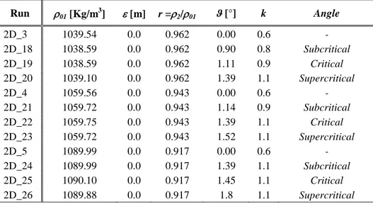
Run x0 [m] h0 [m] 01 [Kg/m3]  [mm] r =2/01 *= /h0 ϑ [°] Angle 2D_1 0.1 0.15 1009.25 0.0 0.991 0.0000 0.00 - 2D_2 0.1 0.15 1023.70 0.0 0.977 0.0000 0.00 - 2D_3 0.1 0.15 1039.54 0.0 0.962 0.0000 0.00 - 2D_4 0.1 0.15 1059.56 0.0 0.944 0.0000 0.00 - 2D_5 0.1 0.15 1089.99 0.0 0.917 0.0000 0.00 - 2D_6 0.1 0.15 1009.15 0.7 0.991 0.0047 0.00 - 2D_7 0.1 0.15 1009.24 2.2 0.991 0.0147 0.00 - 2D_8 0.1 0.15 1008.75 4.5 0.991 0.0300 0.00 - 2D_9 0.1 0.15 1024.06 0.7 0.976 0.0047 0.00 - 2D_10 0.1 0.15 1024.36 2.2 0.976 0.0147 0.00 - 2D_11 0.1 0.15 1023.73 4.5 0.977 0.0300 0.00 - 2D_12 0.1 0.15 1038.90 0.7 0.963 0.0047 0.00 - 2D_13 0.1 0.15 1038.68 2.2 0.962 0.0147 0.00 - 2D_14 0.1 0.15 1039.47 4.5 0.962 0.0300 0.00 - 2D_15 0.1 0.15 1060.56 0.7 0.943 0.0047 0.00 - 2D_16 0.1 0.15 1060.00 2.2 0.943 0.0147 0.00 - 2D_17 0.1 0.15 1059.47 4.5 0.944 0.0300 0.00 - 2D_18 0.1 0.15 1038.59 0.0 0.963 0.0000 0.90 Subcritical 2D_19 0.1 0.15 1038.59 0.0 0.963 0.0000 1.11 Critical 2D_20 0.1 0.15 1039.10 0.0 0.962 0.0000 1.39 Supercritical 2D_21 0.1 0.15 1059.72 0.0 0.944 0.0000 1.14 Subcritical 2D_22 0.1 0.15 1059.75 0.0 0.944 0.0000 1.39 Critical 2D_23 0.1 0.15 1059.72 0.0 0.944 0.0000 1.52 Supercritical 2D_24 0.1 0.15 1089.99 0.0 0.917 0.0000 1.39 Subcritical 2D_25 0.1 0.15 1090.10 0.0 0.917 0.0000 1.45 Critical 2D_26 0.1 0.15 1089.88 0.0 0.917 0.0000 1.8 Supercritical

Table 1: Experimental parameters used to perform 2D gravity currents.

2.1.3. Experimental results

2.1.3.1. Flat smooth bed

In Figure 2.4a-b experimental front’s positions versus time are shown for all the experiments performed on flat smooth bed (i.e. Runs 2D_1-2D_5), in dimensional and dimensionless form, respectively. All the runs shown in this

section are performed keeping constant h0 and x0 and testing five different values of ρ01. The values of the experimental parameters are shown in Table 1. All the laboratory measurements starts about two seconds after the removal of the sliding gate, because it was difficult to measure the profile of the current during its initial stage of development.

Dimensionless front position xf * is defined as: 0 0 * x x x x_f  f  (21)

Dimensionless time T* is defined on the basis of the time scale t0 as:

0 0 0 0 0 ' ; * h g x t t t T   ₍₂₂₎

where g'0 is the initial reduced gravity, given by:

2 2 01 0 ' ρ ρ ρ g g   (23)

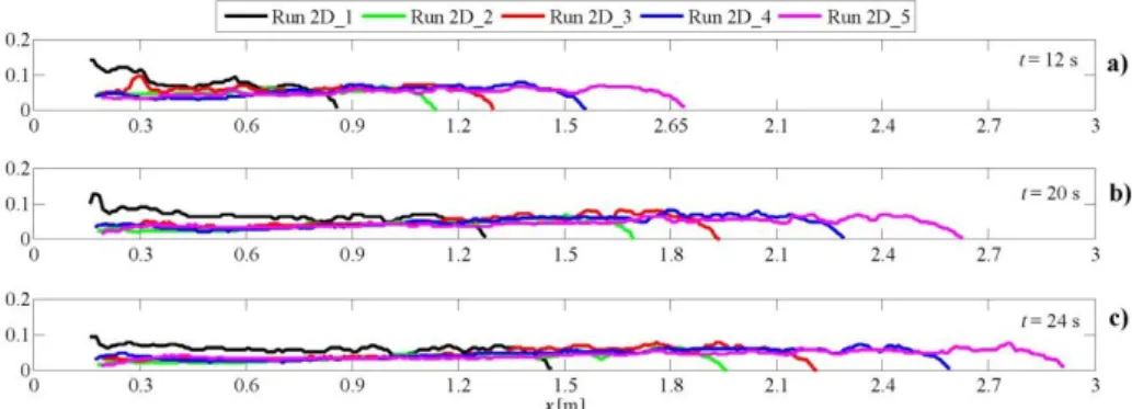
in which g is the gravity acceleration. Figure 2.4a shows that the speed of the current increases as the initial density of released current increases. For a constant time, the gravity current with higher initial density covers a longer distance than those realized with lower values of initial density. Figure 2.4b shows that all the time histories of the front position in dimensionless form of relative to the runs performed with different values of the initial density of the gravity current and keeping constant the other experimental parameters lye all on the same curve. Such a result is in agreement with most of the studies about gravity currents, as Marino et al. 2005. Figure 2.5a-c shows the comparisons of current profiles for all the runs performed on flat smooth bed, at three different time steps after release of the dense fluid, t=12 s (Figure 2.5a), t=20 s (Figure 2.5b) and t=24 s (Figure 2.5c), respectively. As observed in Figure 2.4a, as the initial density of the dense fluid increases, the current’s speed increases.

As explained in section 1.2, Huppert & Simpson (1980) and Rottman & Simpson (1983) showed that three phases can be distinguished in the dynamics of a gravity current produced by an instantaneous release. As they investigated gravity currents moving on flat and smooth beds, in the present work the length of the three phases can be computed only for runs 2D_1-2D_5. The length of the

slumping phase ls can be calculated following Rottman & Simpson (1983) by Equation (5). The distance at which the viscous phase starts l* is calculated following Huppert (1982) by Equation (6). The length of the viscous phase lvis is given by the difference between the total length of the tank and the distance at which the third phase starts. The length of the self-similar phase lss can be obtained by the difference between l* and ls. In Table 2 ls, lss, lvis for runs 2D_1-2D_5 are shown. Run 01 [Kg/m3] ls [m] lss [m] lvis [m] 2D_1 1009.25 1.00 0.82 1.18 2D_2 1023.70 1.00 1.10 0.90 2D_3 1039.54 1.00 1.25 0.75 2D_4 1059.56 1.00 1.39 0.61 2D_5 1089.99 1.00 1.53 0.47

Table 2 Lengths of slumping phase ls, self-similar phase lss and viscous phase lvis for all

the runs performed on flat and smooth beds.

Figure 2.4a-b: Dimensional and dimensionless plots of front position versus time for the

runs 2D_1-2D_5, performed on flat smooth bed with different initial densities.

Figure 2.6 show a comparison between experimental front position versus time of runs that runs 2D_1-2D-5 and theoretical front evolution for the three phases given by previous studies. It can be observed that during the first phase, experimental data are placed on a line with slope 1 (solid line), while during the second self-similar phase are on the line with slope 2/3 (dashed line). The third line (dotted line) has a slope of 1/5 and should be followed by data points

corresponding to the third viscous phase. However, although by using laws from Rottman & Simpson (1983) and Huppert (1982) it can be predicted that runs 2D_1-2D_5 develop the three phases during their evolution, the log-log plot shows in Figure 2.6 shows that these experimental data are in agreement with previous formulae only for the first and the second phase, while the third phase seems not to occur in the current’s evolution. It can be supposed that the length of the viscous phase should be longer than the ones occurring in the dynamics of runs 2D_1-2D_5 in order to be observable in experimental results. Moreover Equation (7) was derived by Huppert (1982), on the basis of some hypothesis, among which the hypothesis of immiscibility of the two fluids, while entrainment phenomena are involved in the gravity currents’ dynamics analyzed in this work, as will be fully shown in section 2.3.3.

Figure 2.5a-c: Measured gravity current’s profiles at three different time steps for the

runs 2D_1-2D_5, performed on a flat smooth bed with different initial densities.

Figure 2.6: Dimensionless log-log plot of front’s position versus time for the runs

performed on flat and smooth beds. Dashed line, solid line and dotted line are the theoretical front evolution for the slumping, self-similar and viscous phase, respectively.