ALMABEST: a new whole building energy simulation Simulink-based tool for NZEB design

(1)

A

l

m

a

M

a

t

e

r

S

t

u

d

i

o

r

u

m

–

U

n

i

v

e

r

s

i

t

à

d

i

B

o

l

o

g

n

a

DOTTORATO DI RICERCA IN

Meccanica e Scienze Avanzate dell’Ingegneria

Ciclo XXXI

Settore Concorsuale: 09/C2

Settore Scientifico Disciplinare: ING-IND/10

ALMABEST: A NEW WHOLE BUILDING ENERGY SIMULATION

SIMULINK-BASED TOOL FOR NZEB DESIGN

Presentata da: Jean Pierre Campana

Coordinatore Dottorato

Supervisore

Prof. Marco Carricato

Prof. Gian Luca Morini

(2)

(3)

(4)

(5)

i

ABSTRACT

In this Thesis the new tool ALMABEST for the dynamic energy simulation of the whole building coupled to HVAC systems is presented. This tool, developed in the Matlab environment, consists of two libraries, ALMABuild and ALMAHVAC, dedicated to the building and HVAC system modelling respectively; this Thesis is focused in particular on ALMABuild.

A large number of software for the analysis of dynamic behaviour of buildings have been proposed and are now available for the designers. For this reason, the reader can have some doubt about the need of a new software for dynamic energy building simulations.

One of the main goals of this Thesis is to demonstrate that ALMABEST presents complementary features with respect to the commercial codes available in the market, which can greatly help the user in the design of new NZEB. In fact, the main features required for the NZEB design (ability to perform multi-objective optimizations, detailed comfort assessments and accurate evaluation of the energy performance of buildings and HVAC systems also in presence of active occupants) are aspects that the codes available on the market only partially are able to manage.

In the first part of this Thesis, the description of ALMABuild, which consists of a Simulink library and a set of Graphical User Interfaces (GUIs), is presented. In particular, the models implemented in the main ALMABuild blocks are explained and the procedure for the creation of the building model by using a series of GUIs is illustrated. It is emphasized how the use of these GUIs allows to overcome the drawback of other Simulink-based tools in terms of introduction of building data and of implementation of the model in the Simulink desktop. The benchmark of ALMABuild has been performed following the BESTEST procedure, adopted for the validation of the main whole building software available in the market. Results of analytical and empirical tests have confirmed the validity of the models implemented in ALMABuild. The same result has been confirmed by the comparative tests made by using a series of reference software under a set of univocally defined cases. The results highlight how the comparison suggested by the BESTES procedure need to be continuously updated by varying the list of the reference software used for comparisons in order to obtain a more updated benchmark and be able to take correctly into account the natural evolution of the building modelling.

In the second part of this work, applications of the ALMABEST tool are illustrated with the aim to highlight the main features of this tool. In particular,

(6)

ii

the detailed evaluation of the spatial distribution of radiative, indoor air and operative temperature obtained by means of ALMABEST has been used in order to compare six different emitters (from radiators to radiant floors) with the aim to put in evidence how the indoor local comfort conditions are influenced by the emitters. Furthermore, the impact of the temperature sensor position in a room on the local indoor comfort conditions and on the dynamic response of the emitters has been analysed.

The coupling of the Matlab Optimization Toolbox with ALMABuild is illustrated by means of a series of single and multi-objective optimizations in which the total annual energy demand is minimized by modifying a series of specific building parameters, like thermal insulation thickness and the total clear area. Results remark the significant improvements of the building energy performance that can be obtained by using this design approach, with energy savings up to 65% with respect to a reference building configuration. The limited number of simulations required by the optimization algorithm to find the optimal solution, even for a large number of possible configurations underlines how these optimization algorithms can be nowadays used during the design of a NZEB with limited computational costs.

Finally, the impact of occupant interactions with the building elements, in particular windows, on comfort and heating energy consumptions is analysed. The effects of the occupant behaviour on the optimal building parameters configuration able to maximize comfort conditions and minimize the energy demand are investigated by means of multi-objective optimizations. A robustness parameter is introduced in order to individuate the main configurations which tend to minimize the role of the occupant on the indoor comfort conditions and on the energy demand (occupant-free configuration). Results emphasize how the presence of occupants and their active behaviour cannot be ignored if an accurate and realistic evaluation of the building performance have to be obtained.

(7)

iii

List of Figures

Figure 1.1 Fraction of energy sources in the residential sector in Europe, in 2016 (from [5]). ... 3

Figure 1.2. Example of elements composing a building-HVAC system, characterised by different time constants. ... 8

Figure 2.1. Simulink library. ... 26

Figure 2.2. Example of a simple model implemented in Simulink. ... 27

Figure 2.3. ALMABEST hierarchical levels. ... 28

Figure 2.4. Plant of a two-stage building. ... 29

Figure 2.5. Simulink model of the two-stage building developed by means of ALMABEST. ... 30

Figure 2.6. ALMABuild library main level. ... 32

Figure 2.7. Example of models that compose a Thermal zone block. ... 33

Figure 2.8. ALMABuild main interface. ... 34

Figure 2.9. Exploded of the Weather Data block of the ALMABuild library. ... 34

Figure 2.10. Exploded of the Climatic Data block for a building characterised by three orientations (East, West, South). ... 35

Figure 2.11. Weather Data Reader block. ... 36

Figure 2.12. Solar Data block. ... 36

Figure 2.13. Solar Radiation Calculator model. ... 38

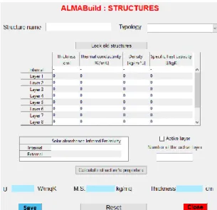
Figure 2.14. Structure GUI used for the definition of main characteristics of massive elements. ... 39

Figure 2.15. Blocks composing the Building Components blockset. ... 42

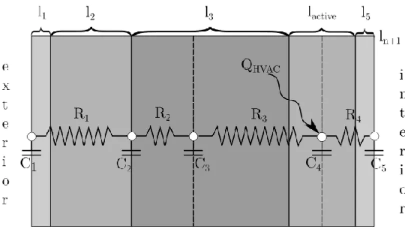
Figure 2.16. Equivalent 3R4C network associated to an opaque envelope building. ... 43

Figure 2.17 Floor on ground RC network. ... 45

Figure 2.18. Equivalent RC network related to an opaque element with an active layer (lactive). ... 45

Figure 2.19. BME block of an external wall. ... 46

Figure 2.20. Window GUI, for the definition of characteristics of clear envelope elements. ... 48

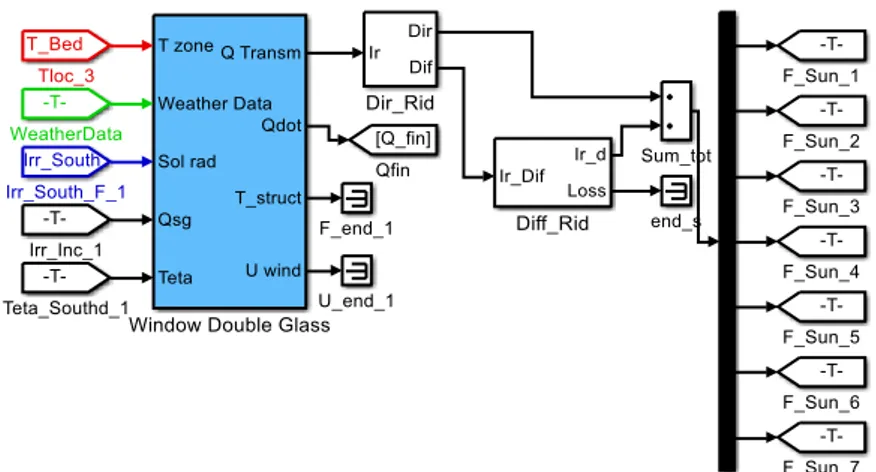
Figure 2.21. BCC block for a double pane window. ... 51

(12)

viii

Figure 2.23. Graphical representation of a building with a horizontal shading device (in grey), obtained by the

ALMABuild shading GUI. ... 54

Figure 2.24. Thermal zone properties GUI. ... 57

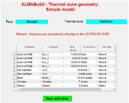
Figure 2.25. GUI for the insertion of the thermal zone geometry for simple model. ... 58

Figure 2.26. Convective star node. ... 60

Figure 2.27. Radiative exchange between three surfaces, delta (a) and star (b) network. ... 61

Figure 2.28. BTB blocks for the evaluation, by means of the simple model, of the temperature of the zone (left block) and of the ideal power for fixed thermal zone conditions (right block). ... 62

Figure 3.1. BESTEST validation scheme. ... 67

Figure 3.2. (a), (b) and (c): Experimental set-up. (1) is the heat flow meter that, together with the Pt1000 RTD sensors (2) and (3), composes the Optivelox Thermozig, (4) and (5) are outdoor and indoor air temperature sensor and (6) is the data acquisition system. ... 70

Figure 3.3. Hourly profile for the incident solar radiation over the wall (a) and of internal heat gains (b) used for the evaluation of the internal wall surface temperature with ALMABuild. ... 70

Figure 3.4. Comparison between the empirical data and the numerical result obtained using ALMABuild in terms of internal surface temperature of the wall. ... 71

Figure 3.5. The reference building geometry indicated by BESTEST for software verification. ... 74

Figure 3.6. Horizontal shading device for cases 610 and 910 (a); vertical and horizontal shading devices for cases 630 and 930. ... 74

Figure 3.7. Hourly incident solar radiation during a clear (higher profile) and cloudy (lower profile) day for: South (a) and West (b) orientation. ... 76

Figure 3.8. Trend of hourly free-floating internal air temperature for Case 600FF (a) and Case 900FF (b): comparison with the BESTEST limits. ... 81

Figure 3.9 Trend of hourly free-floating internal air temperature for case 650FF (a) and case 950FF (b): comparison with the BESTEST limits. ... 82

Figure 3.10. Comparison of the annual energy demand [MWh] predicted by EnergyPlus, the Standard EN 52016 and ALMABuild for lightweight BESTEST buildings. ... 89

Figure 3.11. Comparison of the annual energy demand [MWh] predicted by EnergyPlus, the Standard EN 52016 and ALMABuild for heavyweight BESTEST buildings. ... 90

Figure 3.12. Comparison of the annual power peak [kW] predicted by EnergyPlus, the Standard EN 52016 and ALMABuild for lightweight BESTEST buildings. ... 91

Figure 3.13. Comparison of the annual power peak [kW] predicted by EnergyPlus, the Standard EN 52016 and ALMABuild for heavyweight BESTEST buildings. ... 92

Figure 4.1. Thermal zone properties GUI for the data insertion for the BTB block radiative model. ... 98

Figure 4.2. GUI for the definition of the temperature sensor position and of the spatial discretization, for the radiative model (a) and graphical representation of the inserted data (b). The sensor is represented as the green cube in (b), whilst the grid points are in grey. ... 99

(13)

ix

Figure 4.3. BTB block for detailed radiative model. ... 101

Figure 4.4. Temperature map sub-system. Inputs are the temperature of the inner surfaces of the zone in addition to the temperature zone bus, whereas the outputs are the map of mean radiant and operative temperature distribution within the zone... 102

Figure 4.5. Building Massive Element block for thermal zone described by the radiative model. ... 103

Figure 4.6. Layers between two cells: vertical (a) and horizontal (b). ... 105

Figure 4.7. Pressure difference (ΔP) between cell i and cell j in a vertical layer, if only buoyance forces are considered. The neutral point is located where ΔP is zero... 106

Figure 4.8. BTB block for detailed convective model. ... 108

Figure 4.9. Customized Air Temperature Map block. ... 108

Figure 4.10. BTB block for fully detailed model. ... 109

Figure 4.11. Reference room for the validation of the MATLAB routine for view factors calculation. ... 111

Figure 4.12. (a) Plan of the room with indication of the position of the sensor; (b) Position and size of window and radiator for case A; (c) Position and size of window and radiator for case B and C. ... 114

Figure 4.13. Vertical profile of the operative temperature at the centre of the room for the coldest day of the year when the heaters reach their maximum surface temperature. ... 119

Figure 4.14. Room operative temperature distribution (°C) in the coldest day of the year when the heaters reach their maximum surface temperature, at three levels above the floor (0.1 m, 0.9 m and 1.7 m) in case of low thermal insulation (Case A). ... 121

Figure 4.15. Operative temperature of the room measured in the coldest winter day by the room sensor in presence of different emitters and envelope thermal insulations. ... 122

Figure 4.16. Characteristic time ton (a) and toff (b) for different emitters and for different building thermal insulation, by considering the control system dead band of 19-20.5 °C. ... 123

Figure 4.17. tcomf for emitters (1), (2) and (3), considering both low and high insulated buildings. ... 125

Figure 4.18. tcomf for emitters (4), (5) and (6), considering both low and high insulated building. ... 126

Figure 4.19. Plant view of offices. Comfort zone is evidenced in blue, whilst A, B and C refer to the position of the temperature sensor. ... 127

Figure 4.20. Room discretization in air cells, plant view (a) and height discretization (b). ... 128

Figure 4.21. Cumulative distribution of the operative temperature of the comfort zone. ... 130

Figure 4.22. Operative temperature distribution at 1 m height from the floor, when the indoor temperature reaches the upper value of the control band (20.5 °C). a, b, c refers to the sensor position, highlighted with the red point. The red rectangle represents the comfort area. ... 131

Figure 4.23. Comparison between the operative temperature of the sensor and in the comfort zone, for two typical days of the year. The sensor is in position A (a), B (b) and C (c). ... 132

(14)

x

Figure 4.25. Cumulative distribution of the mean operative temperature of the comfort zone, sensor in position A. ... 134 Figure 4.26. Comparison of the cumulative distribution of the mean operative temperature in the comfort zone, for sensors in position C, with different settings, and Case B. ... 136 Figure 4.27. Cumulative distribution of the mean operative temperature in the comfort zone, for cases R2, for different thermostat sensor position (A, B and C). ... 136 Figure 4.28 Comparison between cumulative mean operative temperature for case B, with inlet water temperature of 80 °C (red solid line) and 60 °C (blue dotted line). ... 137 Figure 4.29. Weather compensation curves for Case R1 and R2. ... 139 Figure 4.30. Cumulative distribution of the mean operative temperature of the comfort zone. ... 139 Figure 4.31. Cumulative distribution of the number of daily on-off cycles of the heating system adopting the weather compensation. ... 141 Figure 4.32. Cumulative distribution of the mean operative temperature of the comfort zone in cases R2 adopting the weather compensation, for different sensor position. ... 142 Figure 4.33. Cumulative distribution of the mean operative temperature in the comfort zone, for fast restart cases. ... 144 Figure 5.1. Example of Pareto Frontier. In red is highlighted the Pareto frontier, composed by points B and C, whilst A represent a dominated solution. ... 152 Figure 5.2. Geometry of the reference building. ... 154 Figure 5.3. Total annual energy demand [MWh] as a function of the insulation thickness of the external walls and roof and of the total clear area. ... 155 Figure 5.4. Ratio between the total energy consumptions and the total energy consumptions for the reference case, as a function of non-dimensional insulation thickness and clear area. The red point indicates the reference case. ... 157 Figure 5.5. Total, heating and cooling annual energy demand as a function of the overhang length. ... 158 Figure 5.6. Annual heating (a) and cooling (b) energy demand [MWh], as a function of insulation thickness and overhang length. ... 159 Figure 5.7. Total annual energy demand as a function of insulation thickness of opaque envelope elements and overhang length. The dotted line is the local minimum curve. ... 160 Figure 5.8. Total energy demand [MWh] as a function of insulation thickness and overhang length for total clear area of 8 (a), 10 (b), 12 (c) and 14 (d) m2_{. ... 161}

Figure 5.9. Local minimum curve: the optimal overhang length is expressed as a function of the total clear area, considering the maximum insulation thickness. ... 162 Figure 5.10. Heating energy demand and mean annual PPD for buildings with windows in both East and West walls (total clear area of 9 m2_{) considering different insulation levels, both in the external and internal}

layers. The filled markers refer to solutions that compose the Pareto frontier. ... 164 Figure 5.11. Heating energy demand and mean annual PPD for buildings characterised by total clear area of 8 m2_{, considering different insulation thicknesses (on the external side of the elements) and various windows}

(15)

xi

Figure 5.12. Indoor operative temperature for a typical winter (a) or summer (b) day, for buildings with two window expositions: East-West (blue solid line) or South (red dashed line). ... 166 Figure 5.13. Pareto frontier for the optimization of mean annual PPD and of heating energy demand. Results concern buildings composed by windows on the South wall; filled markers refer to internal insulation of opaque elements. ... 167 Figure 6.1. Air change rate (ACH) as a function of the absolute temperature difference between indoor and outdoor. ... 175 Figure 6.2. Annual comfort time (tcomf) for different insulation thickness, shadings and windows for cases with

set point temperature equal to 21 °C, neglecting the occupant behaviour. (a) refers to window D1, (b) to window D2, (c) to window D3 and (d) to T1. ... 179 Figure 6.3. Overheating (hot) and undercooling (cold) times for the optimal (highest comfort time) configuration for each window typology. ... 180 Figure 6.4 Annual comfort time for different insulation thickness, shadings and windows for cases with set point temperature equal to 23 °C, neglecting the occupant behaviour. (a) refers to window D1, (b) to window D2, (c) to window D3 and (d) to T1. ... 181 Figure 6.5. Overheating time (thot) for window D2, as a function of insulation thickness and shadings, indoor

set-point temperature of 23 °C. ... 182 Figure 6.6. Relative standard deviation for comfort time (a) and heating energy consumptions (b), for each building configuration, due to the stochastic user behaviour model. ... 184 Figure 6.7. Annual comfort time (tcomf) for different insulation thickness, shadings and windows in cases with

set point temperature equal to 21 °C, considering the occupant behaviour. (a) refers to window D1, (b) to window D2, (c) to window D3 and (d) to T1. ... 186 Figure 6.8. Overheating (hot) and undercooling (cold) times for the optimal (highest comfort time) configuration for each window typology, considering occupant behaviour. ... 187 Figure 6.9. Annual comfort time (tcomf) for different insulation thickness, shadings and windows in cases with

set point temperature equal to 23 °C, considering the occupant behaviour. (a) refers to window D1, (b) to window D2, (c) to window D3 and (d) to T1. ... 187 Figure 6.10. Overheating time (thot) for buildings characterised by window D1, shading Sh2 and set-point of

21 °C as a function of insulation thickness, both considering and neglecting the occupant behaviour. ... 189

Figure 6.11. Comfort time sensitivity to insulation (S_{comf i}_, ) considering (blue bars) or neglecting (green bars) the occupant behaviour, for different shadings and windows: (a), (b), (c) and (d) refer to window D1, D2, D3 and T1, respectively. ... 191

Figure 6.12. Comfort time sensitivity to shadings (S_{comf sh}_, ) considering (blue bars) or neglecting (green bars) the occupant behaviour, for different insulations and window: (a), (b), (c) and (d) refer to window D1, D2, D3 and T1, respectively. ... 192

Figure 6.13. Comparison of S_{E i}_, for different shadings and windows: (a), (b), (c), (d) refers to windows D1, D2, D3 and T1, respectively. ... 193

Figure 6.14. Sensitivity of energy demand on shadings S_{E sh}_, , both considering (blue bars) and neglecting (green bars) the occupant behaviour, for different insulations and windows D1 (a), D2 (b), D3 (c) and T1 (d). ... 194

(16)

xii

Figure 6.15. Pareto frontiers of multi-objective optimizations for different window typologies, referring to buildings with set point of 21 °C. (a) refers to buildings composed by window D1, (b) to buildings with windows D2, (c) to cases with window D3 and (d) to window T1 cases. ... 196 Figure 6.16. Pareto frontiers of multi-objective optimizations for different windows typology, referring to buildings with thermostat set point equals to 23 °C. (a) refers to buildings composed by window D1, (b) to buildings with windows D2, (c) to cases with window D3 and (d) to window T1 cases. ... 198 Figure 6.17. Pareto frontiers of multi-objective optimizations referring to buildings with thermostat set point equals to 21 °C (a) and 23 °C (b). ... 199 Figure 6.18. Sensitivity to the occupant behaviour of optimal building configurations for each window typology. ... 202 Figure 6.19. Maximum number of window openings for specific window and shading configurations. ... 202

(17)

xiii

List of Tables

Table 1-1. Main features of ESP-r, EnergyPlus and TRNSYS. ... 14

Table 1-2. Main features of Simulink toolboxes for building performance simulation. ... 21

Table 2-1. ALMABuild bus signals. ... 31

Table 2-2. Optical window properties. ... 48

Table 2-3. Gas gap properties ... 48

Table 2-4. Glass properties. ... 49

Table 2-5. Frame properties. ... 49

Table 3-1. Wall stratigraphy for the room considered in the ALMABuild analytical verification. ... 68

Table 3-2. Comparison between analytical [103] and numerical values of the indoor air temperature (in °C) obtained with ALMABuild. ... 68

Table 3-3. Stratigraphy of the measured wall. ... 69

Table 3-4. List of the qualification cases analysed during the comparative tests. ... 73

Table 3-5. Annual incident solar radiation [kWh/(m2_{year)] on the external walls of the building of Figure 3.5} obtained by using the reference software and ALMABuild. ... 75

Table 3-6. Annual solar radiation [kWh/(m2_{year)] transmitted by the reference windows, and its mean annual} transmissivity coefficient. ... 77

Table 3-7. Annual solar radiation [kWh/(m2_{year)] transmitted by the reference shaded windows, and the} mean annual shading factor. ... 79

Table 3-8. Annual internal air temperature values (°C) obtained for free-float (FF) BESTEST cases compared with the minimum and maximum threshold values indicated by BESTEST. ... 80

Table 3-9. Annual Heating Load (MWh) obtained for non-free-float lightweight BESTEST cases compared with the minimum and maximum threshold values indicated by BESTEST. ... 83

Table 3-10. Annual Cooling Load (MWh) obtained for non-free-float lightweight BESTEST cases compared with the minimum and maximum threshold values indicated by BESTEST. ... 83

Table 3-11. Annual Heating Load (MWh) obtained for non-free-float heavyweight BESTEST cases compared with the minimum and maximum threshold values indicated by BESTEST. ... 84

Table 3-12. Annual Cooling Load (MWh) obtained for non-free-float heavyweight BESTEST cases compared with the minimum and maximum threshold values indicated by BESTEST. ... 84

Table 3-13. Annual Heating Peak (kW) obtained for non-free-float lightweight BESTEST cases compared with the minimum and maximum threshold values indicated by BESTEST. ... 85

(18)

xiv

Table 3-14. Annual Cooling Peak (kW) obtained for non-free-float lightweight BESTEST cases compared

with the minimum and maximum threshold values indicated by BESTEST. ... 85

Table 3-15. Annual Heating Peak (kW) obtained for non-free-float heavyweight BESTEST cases compared with the minimum and maximum threshold values indicated by BESTEST. ... 86

Table 3-16. Annual Cooling Peak (kW) obtained for non-free-float heavyweight BESTEST cases compared with the minimum and maximum threshold values indicated by BESTEST. ... 86

Table 3-17. Annual heating and cooling load [MWh] and peak [kW] for back zone of Case 960, compared with the minimum and maximum threshold values indicated by BESTEST. ... 87

Table 3-18. Discrepancy [%] between the maximum and minimum BESTEST threshold values for all the qualification tests. Highest and lowest discrepancies are evidenced in bold. ... 88

Table 3-19. Specific heat capacity of massive envelope elements, according to EN 52016 [62]. ... 93

Table 3-20. Classification of elements by mass distribution, according to EN 52016 [62]. ... 93

Table 3-21. Distribution of the element capacity to the RC network node, according to EN 52016. ... 93

Table 3-22. List of validation tests performed and ALMABuild blocks (recalling the section in which are described) involved for each test. ... 94

Table 4-1. Computing runtime for annual dynamic simulations of buildings in free-float conditions, adopting dfferent kind of models. Simulations are performed with a desktop computer with a quad-core 3.40 GHz processor and 8 GB of RAM. The multizone building is composed by four thermal zones. ... 110

Table 4-2. View factors obtained with TRISCO, COMSOL and ALMABuild for the reference room, referring to surface labelled in Figure 4.11. ... 112

Table 4-3. Thermo-physical properties of the main envelope elements. ... 114

Table 4-4: List of radiant and convective heat emitters considered in numerical simulations. nel is the number of element composing the radiator. ... 115

Table 4-5. Radiative power share for the different heaters. ... 117

Table 4-6. Convective (Ta) and mean radiant temperature (Trad) when the room sensor measures an operative temperature of 20.5 °C, during the coldest day of the year, as a function of the adopted heat emitters with a low building thermal insulation level (case A). ... 117

Table 4-7. Inner surface temperature (°C) distribution in the room when the emitters reach their maximum surface temperature (Tem,max) during the coldest day of the year as a function of the thermal insulation level (A or B) and of the adopted emitter. ... 118

Table 4-8. Maximum specific emitted thermal power as a function of emitter and of thermal insulation level. ... 123

Table 4-9. U-values of building elements. ... 128

Table 4-10. Comfort and overheating time (tcomf and thot) in the comfort zone for different position of the sensor. ... 130

Table 4-11. Control system dynamics and energy demand with different sensor position (A, B, C). ... 133

(19)

xv

Table 4-13. Comfort parameters for cases with radiator water inlet temperature of 60 °C. ... 137

Table 4-14. Control parameters for cases with radiator water inlet temperature of 60 °C, and comparison (Δ) with case R1. ... 138

Table 4-15. Comfort and overheating time (tcomf and thot) in comfort zone adopting the weather compensation. ... 140

Table 4-16. Control parameters for cases with weather compensation. ... 140

Table 4-17. Comfort parameters for cases R2 with weather compensation, for different sensor position, and comparison (Δ) with results obtained for radiator R1. ... 142

Table 4-18. Control parameters for cases R2, for different sensor position, and comparison (Δ) with cases R1, considering the weather compensation. ... 143

Table 4-19. Comfort and overheating time for fast restart cases, and comparison to cases without fast restart strategy, Case R2. ... 144

Table 4-20. Control parameters for fast restart cases, sensor in different positions, and comparison to cases without the adoption of the fast restart strategy, Case R2... 145

Table 5-1. Thermal transmittance values of the envelope elements in the reference case. ... 154

Table 5-2. Main characteristics of a radiator element. ... 163

Table 5-3. Constant parameters for the evaluation of indoor comfort conditions. ... 163

Table 6-1. Main characteristics of a radiator element. ... 174

Table 6-2. Thermal transmittance of external opaque envelope elements for different thermal insulation thicknesses. ... 176

Table 6-3. Characteristics of the analysed windows. ... 176

Table 6-4. Shading factor for different overhang geometries. ... 177

Table 6-5. Annual heating energy consumptions [MWh/y], for cases with set-point temperature equal to 21 °C, for different shadings, insulation thicknesses and windows. For each window, minimum energy demand is highlighted on bold. ... 177

Table 6-6. Heating energy demand [MWh/y], for cases with high set-point, varying shadings, insulation and windows, neglecting the occupant behaviour. For each window, minimum energy demand is highlighted on bold. ... 183

Table 6-7. Heating energy consumptions [MWh/y], for cases with set-point temperature equal to 21 °C, for different shadings, insulation thickness and windows, considering the occupant behaviour. For each window, minimum energy demand is highlighted on bold. ... 185

Table 6-8. Heating energy consumptions [MWh/y], for cases with set-point temperature equal to 23 °C, for different shadings, insulation thickness and windows, considering the occupant behaviour. For each window, minimum energy demand is highlighted on bold. ... 188 Table A-6-9. List of tools from the BEST directory [14]. ... A-2

(20)

xvi

Table B- 2. Component of the Sun bus. ... B-2 Table B- 3. Components of the Power Bus. ... B-3 Table B- 4. Components of the Ventilation bus. ... B-3

Table C- 1. List of blocks of the Climatic Data blockset. ... C-2 Table C- 2. List of Building Massive Element blocks, for thermal zone described by means of the simple model. ... C-3 Table C- 3. List of Building Massive Element blocks adopted if the radiative model is used for the description of the thermal zone, for non-active envelope elements. ... C-6 Table C- 4. List of Active Building Massive Element blocks. ... C-11 Table C- 5. List of blocks composing the Building Clear Component subsystem. ... C-16 Table C- 6. List of Building Thermal Balance blocks, for both temperature and ideal power evaluations. . C-19 Table C- 7. Additional blocks used for the description of a thermal zone. ... C-22

(21)

i

Nomenclature

Roman letters

A Area

AM Relative optical air mass c Specific heat capacity C Total heat capacity Cd Discharge coefficient cp Specific heat capacity d Wall layer thickness

D Radiosity

E Energy

F View factor

Fr View factor between external component and sky g Gravitational acceleration

h Heat transfer coefficient H Solar radiation

l Wall layer

m Mass flow

N Nodes of RC models nl Number of wall layers Nu Nusselt number

P Pressure

PPD Predicted Percentage of dissatisfied Prob Probability

Q Power

Ra Rayleigh number S Sensitivity

SF Mean annual shading factor SG Solar gain

SH Shading factor

t Time

T Temperature

U Thermal transmittance

Wop Number of window openings x Position on a layer

(22)

ii

Greek letters

α Solar absorbance β Slope of a surface

γ Azimuth angle of a surface δ Solar declination

Δ sky's brightness ϵ sky's clearness

εs Surface emissivity



Sensitivity of an objective function vector θ Angle of incident of solar radiation λ Thermal conductivity μ Mean values



Albedo  _Density σ Standard deviation σ0 Stefan-Boltzmann constant τs Solar transmissivity

τc Time constant of the i-th element Φ Latitude of a location

φsky Radiative thermal flux with the sky per unit area Ψ Sola elevation angle

ω Solar hour angle

Subscripts

a air

b direct component of incident solar radiation bh beam radiance component on horizontal plane

C referred to the position in which the first quarter of the total thermal capacity of a wall is reached

Cd conduction

comf comfort conv convection

d diffuse component of incident solar radiation dh diffuse radiance component on horizontal plane disc discomfort

e external condition

em emitter

et extraterrestrial

(23)

iii

g ground

hot Occupant comfort state hot is referred to the insulation layer

m mean value

off related to time periods in which the heating system is off on related to time periods in which the heating system is on op operative temperature

opaque opaque envelope element rad radiative heat transfer

refl reflected radiance component rmo running mean outdoor

roof roof

se external surface sg solar gain

sh shaded

si inner surface

sky long-wave radiative heat transfer with the sky sol related to solar radiation

unsh unshaded

w window

(24)

(25)

CHAPTER

ONE

1 Context and Objective

Abstract

In this Chapter, the main motivations of this work are presented. Firstly, the concept of dynamic energy simulation is introduced and the main features of tools for dynamic energy simulations of buildings and HVAC systems required by NZEB designers are described. Analysing three of the most popular Whole Building Energy

Simulation (WBES) software available in the market, i.e. TRNSYS, ESP-r and

EnergyPlus, the main features and limitations of these tools are evidenced.

Then, the features of Matlab/Simulink as framework for developing new WBES tools are discussed with the aim to demonstrate that the Matlab framework can overcome the limitations of many available WBES tools. In particular, the possibility to use all the Matlab toolboxes for solving problems concerning different issues (e.g. optimizations, CFD…) in a single computational environment, avoiding the need of coupling different software packages as well as the possibility to adopt a variable time step discretization for simulations are some of the most attractive features of Matlab for the development of new WBES tools. Therefore, the existing libraries based on Matlab/Simulink for building energy performance simulation are examined, emphasizing the main drawbacks that limited their diffusion up to now.

Finally, the outline of the Thesis, focused on the development of a new Matlab tool for the dynamic energy simulation of buildings and HVAC systems, is presented.

(26)

2

1.1 General context

In the last century, the economic growth and the improvement of living conditions have been accompanied by the explosion of the world energy demand, mainly characterised by the exploitation of fossil fuels like carbon, oil and natural gas. However, the exploitation of fossil fuels has two important drawbacks: the finiteness of the available resources and the negative impact on the environment (pollution and climate change).

For these reasons, in the last two decades, a series of International Agreements, like the Kyoto Protocol [1] and the Paris Agreement [2], have been concluded with the aim to limit the rise of the global temperature up to 1.5°C - 2°C, reducing the primary energy demand and encouraging the exploitation of clean and Renewable Energy Sources (RES). In Europe, the so called 20-20-20 targets reveal the great effort of the European Union (EU) to reduce the negative environmental effects due to fossil fuel exploitation. In fact, by means of the 20-20-20 targets, reported in the Directive 2009/29/EC [3], the EU imposed a 20% reduction of the GreenHouse Gas (GHG) emissions and of the energy consumptions with respect to the values measured in 1990 and a 20% of the RES share on the final energy consumption, by 2020. More restrictive targets have been established by EU for the following years, with the aim to move toward a competitive low carbon economy in 2050 [4]: in this scenario, mid-term targets have been imposed to be achieved by 2030 in the 2030 Climate and Energy Policy Framework [5]: 40% reduction of GHG emissions, compared to 1990 level, the increase of the energy efficiency at least of 27% and the RES share up to 27%.

Residential and service sectors can play an important role for the reduction of energy consumptions and GHG emissions, since they are responsible of about 34% of the global energy consumption [6]. Focusing on Europe, in 2016 the final energy consumption of the residential and service sectors has been of 434 MToe, corresponding to 40% of the total energy consumptions [7]. In Figure 1.1, it is possible to appreciate that around half of the energy used by the residential sector is provided by fossil fuels and only 16% comes from RES [7].

From these data, it is clear that important measures have to be taken, in order to achieve the European targets in the next years. In fact, in the last ten years, EU published a series of Directives, for encouraging the adoption of RES systems, enhancing the building energy efficiency and reducing the use of fossil fuels, for both new and current buildings. The European Directive 2010/31/EU [8], known as the Energy Performance of Building Directive (EPBD), contains the definitions of minimum level of energy performance for building and heating, cooling and ventilation (HVAC) systems for both new and current buildings, according to the “cost optimal approach”. Moreover, EPBD 2010 imposes to the Member States (MS) the transition toward the Nearly Zero Energy Building (NZEB) for new

(27)

1.2 - NZEB design

3

buildings within 2020. In 2012 EU issued the Energy Efficiency Directive (EED) [9] that imposes a renovation rate of at least 3% for the building stock of central governments of MS, since the current renovation rate in Europe is close to only 1% [10], whilst it has been recognized that around 97% of the European building stock has to be renovate in order to achieve a decarbonised building stock by 2050 [11].

Figure 1.1 Fraction of energy sources in the residential sector in Europe, in 2016 (from [5]).

1.2 NZEB design

Even if there isn’t a unique, harmonised concept of NZEB across the MS, EPBD 2010 defines NZEB as buildings characterised by a very high energy performance, in which the very low energy needs are mainly covered by RES. These goals cannot be achieved using classical design strategies, based on a quasi-stationary calculation approach, by means of which energy consumption assessments are obtained considering monthly mean conditions. In fact, NZEB can be designed only by means of a detailed evaluation of the effect of shadings, of the different thermal inertia of building elements, of the internal gain profile and the occupant behaviour (e.g. windows operation, thermostat set-point control) on the energy needs of a building. In addition, the designers must be able to characterise properly RES systems, whose performance strongly depends on variable external conditions (i.e. heat pumps performances depend on the external air temperature and humidity, photovoltaic systems or thermal solar collectors by the incident solar radiation and so on). Besides, the adoption of multi-sources heat generators able to use different energy sources, introduces the problem of the automatic selection of the generation system that, in a specific moment, is able to guarantee the highest performance or the minimum costs or

(28)

4

the highest exploitation of RES, according to different control strategies. In all these cases, a quasi-stationary calculation approach becomes inadequate for the prediction of global energy needs of NZEB.

For these reasons, during the last decade more and more designers are moving from a quasi-stationary approach to a dynamic one for the energy modelling of buildings. Actually, dynamic simulations can be used for the evaluation of passive behaviour of a building, predicting the hourly profile of the internal temperature in free-running conditions (with no HVAC system in operation), as an example.

The design phase of a NZEB requires also a detailed comfort assessment; in fact, energy savings should not lead to a reduction of indoor comfort conditions. On the contrary, optimal design solutions have to be found in order to save energy improving, at the same time, indoor comfort conditions, as it can be done by eliminating overheating/undercooling periods during the year.

It is clear how NZEB design requires the research of a trade-off between energy savings, indoor comfort conditions and economical convenience, that leads the designer to the optimisation of two or more conflicting goals. Multi-objective optimisation can help the designer to comply with these goals, giving the important feedbacks about the selection of envelope elements and HVAC components.

1.3 Dynamic Energy Simulations

The building dynamic energy simulation is an advanced calculation tool based on specific numerical models by means of which detailed information about the thermo-energetic behaviour of the whole building-HVAC system can be obtained. Dynamic simulations are able to give to the designer an accurate reconstruction of the time variation of thermal loads obtained by using adequate time steps, thanks to the introduction of a large amount of input data:

• geometrical information, from orientations and area of each envelope component for the simplest model to the coordinates that define each building component in a three-dimensional cartesian space, required in detailed models in which the internal radiative heat transfer is evaluated by means of view factors;

• thermophysical properties (i.e. thermal conductivity, density, specific heat capacity, water vapour permeability...) of each layer of massive envelope element like walls, roofs and floors;

• windows properties: optical and radiative glass properties, thermophysical data for the gas contained in windows cavity and for the frame;

(29)

1.3 - Dynamic Energy Simulations

5

• thermal zone user profiles: occupancy, internal gains, ventilation profiles, indoor temperature set-up schedule;

• performance maps of each HVAC component (look up tables);

• weather data, like external temperature, vapour pressure, external humidity ratio, wind velocity and direction, solar radiation collected with hourly or sub-hourly frequency.

Contrary to dynamic simulations, models based on a quasi-stationary approach require less input data: as an example, external conditions are described by monthly mean values, whilst for envelope elements only the thermal conductivity is considered among the thermophysical properties. The typology and the number of input data required by quasi-stationary models are described in several National Standard, like the UNI TS 11300 in Italy, where standard profiles for ventilation and internal heat gains can be found.

On the contrary, for the dynamic approach, up to date there is the lack of a Standard which defines the minimum input data required and where some standard schedule for the main user profile can be found (in Italy there is only a draft for a new Standard focused on the base assumptions for building dynamic energy performance simulations [12]). Moreover, it has to be remarked that all the input data required by models based on quasi-stationary approach can be got from technical data sheet, whilst for dynamic models this does not happen. A common example of this lack of information is represented by the window: for its description several dynamic models require information about the angular dependencies of the optical properties, but in common data sheet only aggregate or mean values are reported, that are enough for quasi-stationary models. This lack of standardization of the input data needed by dynamic models leads to two important drawbacks:

• Uncertainty of the building description, due to the lack of information; • Variability of the input data required by different dynamic models. In quasi-stationary simulations, internal conditions (i.e. air temperature) in quasi-stationary simulations are constant input data and from these input data monthly energy consumption and energy losses through the building are estimated. On the other hand, in dynamic simulations internal conditions are not input data, but they are calculated as response to the external and internal (due to HVAC, presence of people, internal gains…) loads; the evaluation of internal conditions is possible thanks to the adoption of short time steps and a correct evaluation of the thermal inertia of the massive building elements in the energy balance equations. In addition, it has to be remarked that in dynamic simulations several physical phenomena (i.e. conductive, convective and radiative heat transfer, mass transfer…) are taken into account together.

As for input data, dynamic simulations are characterised by a huge number of outputs by means of which the dynamic behaviour of the simulated building-HVAC system is described. The main outputs of a dynamic simulation are:

(30)

6 • Air temperature of the thermal zone;

• Surface temperature of each envelope component; • Thermal fluxes of each envelope component;

• Occupant thermal comfort indexes (i.e. Predicted Mean Vote and Predicted Percentage of Dissatisfied [13]);

• Instantaneous values of solar shadings;

• Thermal power released by the HVAC system to the thermal zone.

Due to important simplifications which characterise quasi-stationary simulations, this approach is typically used for the estimation of the energy consumption of a building considering fixed conditions, with the aim to obtain a building energy performance certificate. On the contrary, dynamic simulations are used for voluntary certifications, like LEED (Leadership in Energy and Environmental Design) certificate developed by the U.S. Green Building Council, which considers all the aspect of a building (e.g. economic issues, water consumption, indoor air quality, energy consumption and GHG emissions) and it is used for ranking energy and water efficient, healthy, environmentally-friendly cost saving buildings. Moreover, dynamic simulations are adopted each time it is required to analyse the behaviour of the building-HVAC system in particular conditions or for making energetic diagnosis or in the design of high energy performant buildings or refurbishments.

1.4 Dynamic Energy Simulation Tools

In section 1.2, the three main characteristics of the NZEB design have been highlighted:

• Adoption of a dynamic approach instead of the quasi-stationary one for the analysis of the energy performances;

• Detailed comfort assessment;

• Multi-objective optimisation issues (comfort, cost, energy savings).

In order to help the designer to comply with these new goals, a great number of tools has been developed in the last years. In the Building Energy Simulation Tools (BEST) directory, previously managed by the Department of Energy of the United States and now under the control of the International Building Simulation Association (IBPSA), a list of 181 software tools can be found [14]. The BEST’s directory enumerates tools related to the building energy performance assessment; as reported in Appendix A, where the tools collected in BEST’s directory are listed (except the training and support service tools), these tools have different capabilities. Not all these tools are able to perform an energy performance assessment, some of them are related to the weather data analysis and they are used for making these data available for other software; other tools are used for collecting data for performing building energy audit, for enabling

(31)

1.4 - Dynamic Energy Simulation Tools

7

parametric and optimisation analysis or for making air flow or detailed component simulations. Moreover, two kinds of software able to carry out the evaluation of the energy performance of a building can be found in the BEST’s directory: one is based on dynamic simulations of the whole building-HVAC system (Whole Building Energy Simulation, WBES, software), the other is based on energy bills analysis.

Among all these tools, the most interesting for NZEB design are the WBES, a little fraction of all the tools reported in the BEST’s directory. These tools are used for the prediction of the temporal evolution, under unsteady boundary conditions, of several physical parameters, enabling energy dynamic simulations. In this way, detailed information about the dynamic behaviour of the building coupled with its HVAC system are available and the evaluation of the impact of energy savings measures can be accurately analysed. The main differences among the WBES are related to:

• The list of the physical phenomena accounted for (i.e. shading effects, natural or mixed ventilation, air moisture transport/buffer, illuminance and so on);

• The kind of the adopted modelling (i.e. modelling based on lumped parameters, finite volume or transfer functions);

• The solver scheme (i.e. minimum time-step allowed, 2- or 3-dimensions geometry models and so on);

• Ability to model complex control systems;

• Possibility to evaluate occupant comfort and behaviour.

Generally, WBES tools do not allow a detailed prediction of comfort conditions, since the complete control of the local indoor conditions of a thermal zone needs a detailed reconstruction of the spatial distribution of humidity ratio, radiant temperature and air velocity among other parameters. To obtain this goal, a complete Computational Fluid Dynamics (CFD) simulation is generally needed, with an increase of the computational cost of the whole simulation which is obtained by coupling CFD and WBES by introducing the “co-simulation” concept. This concept describes simulations in which two or more software platforms are combined together with the aim to obtain detailed information about the observed system. For these reasons, another important feature required to WBES tools for being used for NZEB design is the ability to share information during the run-time simulation process with other software: in this way, not only detailed comfort assessment can be made (i.e. by coupling WBES tool with CFD), but also different WBES tools able to analyse only single physical phenomena could be coupled together and used for NZEB design.

Co-simulation is used also for solving multi-objective optimization problems, very frequent in the design of NZEB: in fact, WBES tool in some cases is not directly able to use optimisation algorithms. In these cases, multi-objective optimisation is obtained by using a specific external software (like

(32)

8

modeFRONTIER [15]) in order to drive the WBES tool through the optimization. By means of the optimisation algorithm implemented in a dedicated software, input data of dynamic simulations performed with WBES tool can be iteratively modified, until optimal solutions are found.

1.5 Time step discretization

The dynamic approach consists in the description of several physical phenomena by means of transient balance equations. The accuracy of the solution of these equations depends on the time step discretization adopted, that is related to the time constant of the analysed system.

As represented in Figure 1.2 a building is composed by a series of elements, like walls or roofs (indicated as 1 and 2), windows (3) and HVAC components (4 and 5), which are described by different transient equations.

Figure 1.2. Example of elements composing a building-HVAC system, characterised by different time constants.

Generally, in a dynamic model, a transient equation related to i-th component of a building or HVAC system has the following generalized expression:

= − + i i i i dT B T C dt (1.1)

In this equation, T_i represents the dependent variable of interest, whilst Bi and i

C are coefficient not depending from Ti. As an example, equation (1.1) can

describe the air thermal balance in a thermal zone; in this case Ti is the air

temperature of the zone, Bi is the global heat transfer coefficient over the air

thermal capacity and Ci represents the thermal fluxes not depending on the air

temperature, like internal gains or solar radiation, scaled on the air thermal capacity.

(33)

1.5 - Time step discretization

9

The general solution of equation (1.1) can be expressed as the linear combination of the solution associated to the homogeneous equation and a steady-state particular solution of (1.1) as:

− = B ti + i i i i C T A e B (1.2)

where Ai is a constant that can be determined by means of an initial condition on i

T. From this equation, the time constant of the system,  , can be derived as ci 1 Bi

.

The time constant indicates the characteristic time interval during which the system is able to react to a variation of its thermal conditions. Following the previous example, for the thermal balance of the air of a thermal zone the time constant is given by the ratio between the air capacity and the total heat loss coefficient. A similar equation is obtained for the dynamic analysis of massive envelope elements; again, the time constant of the element is given by the ratio between its thermal capacity and its thermal transmittance.

However, referring to the two examples described, even if the time constants have the same definition, as the thermal capacity of the massive element is at least three or four order of magnitude higher than that of the air, whilst heat loss coefficients are of the same order of magnitude, time constants assume very different values. In fact, the time constant related to the heat transfer that affects the air in the thermal zone is on the order of minutes, whilst heat transfer across massive elements has characteristic time interval of the order of hours. Therefore, a dynamic model of a building is composed by a set of very different time constants (one for each element of the analysed system): indoor air temperature has a time constant of minutes, the massive elements of hours, and HVAC elements, like thermostatic valves, are described by time constants of seconds.

As the time constant is a measure of the characteristic time interval of the considered physical phenomenon, accurate dynamic simulations, which are able to take into account all the dynamic phenomena involved in a building, must be obtained by considering a time step discretization lower than the smallest time constant of the whole system.

Due to the important discrepancy among the time constants involved in the building-HVAC system description, building models based on the dynamic approach can be solved in different ways, depending on the features of the numerical solver adopted. In detail, numerical solvers are characterised by the typology of time step (constant or variable) that are able to manage and by the ability to solve in a single environment several equations adopting different time steps for each equation.

(34)

10

Numerical solvers that adopt the same, constant time step discretization for the solution of the ordinary differential equations are the simplest. In this case, accurate solutions are obtained if the constant time step is less or of the order of magnitude of the lower time constant (which describes the fastest phenomenon). Nevertheless, usually the time step allowed by the solvers have a lower limit, which can depend on the models used for the building description. Moreover, it has to be remarked that, the lowest is the time step, the higher is the simulation time. For this reason, constant time steps are usually hourly or sub-hourly, making models based on this kind of solver not suitable for the simulation of building coupled with controlled HVAC system.

More complex solvers allow the use of variable time step. In this case, the solver refines the solution reducing the time step discretization if necessary, i.e. when faster phenomena became dominant on the other slower phenomena. As an example, when the HVAC system is off, the solver can adopt a time constant of few minutes, in order to evaluate correctly the internal air temperature variations, but when the HVAC system is on and the thermostatic valves open, the solver must be able to refine the solution adopting a time constant of seconds, in order to describe accurately the transient of the fastest phenomenon generated by the valve operation. In this way, accurate simulation of the whole building-HVAC system can be obtained with reasonable simulation time and by assuring accurate results.

Finally, some numerical solvers are able to solve different equations with different time step in the same numerical environment. Usually, this typology of solvers adopts two different time step discretization and equations are divided in two categories as a function of their time constant: equations related to slow transients are solved with the higher time step, whilst the remaining equations (concerning the HVAC system) with the lower one. By means of this kind of solver, between two consecutive time steps for the slow transients, fast transients are evaluated several times. In this way, the simulation time is lower than if a single time step is considered, but the solution may be less accurate, due to the fact that the coupling between building and HVAC system is simplified, as the equations related to the building and the HVAC systems are solved with different time steps.

1.6 Description of the main WBES tools

After having listed the main characteristics required to a WBES tool for the NZEB design and having described different numerical solvers adopted for the solution of set of transients, three specific WBES tools, very diffuse in the thermal engineering community, are described (ESP-r, EnergyPlus, TRNSYS) in order to highlight their peculiarities and their suitability for NZEB design.

(35)

1.6 - Description of the main WBES tools

11

1.6.1 ESP-r

ESP-r is an open-source software, created in 1974 by the University of Strathclyde, for the building energy performance modelling. ESP-r is a whole building simulation software that enables the analysis of the interactions between envelope, external conditions, air flows, HVAC, control systems and comfort conditions of a building [16]. In ESP-r, each physical domain is analysed sub-dividing it in several sub-volumes, each of them described by mass, momentum and energy conservation equations. The domain sub-division is controlled by the user, defining different detail levels. In this way, in the early design phase, a thermal zone could be analysed as a single volume, in which air is perfectly mixed, whilst in more advanced design phases more sub-volumes could be considered for the same zone enabling the evaluation of air stratification in the zone. Increasing considerably the number of sub-volumes used for the description of a thermal zone, CFD analysis is possible, adopting also models for the descriptions of air turbulent flows (e.g. k-ε model).

Finite difference method is adopted also for the HVAC system modelling. Again, HVAC components can be modelled by means of a single volume or with a higher number of volumes. Models of the main HVAC systems (solar [17], air conditioning [18]- [19] or cogeneration plants [20]- [21]) can be found in the ESP-r Database.

In ESP-r, the equations set describing all the physical phenomena considered (conduction, radiative heat transfer, air flows…) is processed simultaneously [22]. However, the different domains of a building are characterised by different time constants (i.e. envelope elements with higher thermal inertia and higher time constant compared to HVAC components). For reducing the simulation time, in ESP-r the modular solver uses different, but constant, time steps for solving building and HVAC system models. In this way, as an example, the energy balance equations of a thermal zone can be solved adopting an hourly time step, and within this time step, the state of the sub-systems characterized by time constants lower than 1 hour (i.e. HVAC systems) are evaluated a different number of times depending on the value of their time constant.

Multi-objective optimisation problems can be solved using ESP-r, but only coupling it to another software that contains optimisation algorithms, as demonstrated by Padovan and Manzan [23], who coupled the modeFRONTIER optimisation tool with ESP-r for the optimisation of a PCM enhanced storage tank in a solar domestic hot water system.

1.6.2 EnergyPlus

EnergyPlus is a modular, open-source software for the building energy performance modelling, created in 2001 and based on the more detailed sub-routines of two other WBES tools: DOE-2 and BLAST, developed by the US