2020-12-03T12:16:09Z
Acceptance in OA@INAF
The ALMA Spectroscopic Survey in the HUDF: the Molecular Gas Content of
Galaxies and Tensions with IllustrisTNG and the Santa Cruz SAM
Title
Popping, Gergö; Pillepich, Annalisa; Somerville, Rachel S.; DECARLI, ROBERTO;
Walter, Fabian; et al.
Authors
10.3847/1538-4357/ab30f2
DOI
http://hdl.handle.net/20.500.12386/28646
Handle
THE ASTROPHYSICAL JOURNAL
Journal
882
The ALMA Spectroscopic Survey in the HUDF: the Molecular Gas Content of Galaxies
and Tensions with IllustrisTNG and the Santa Cruz SAM
Gergö Popping1 , Annalisa Pillepich1 , Rachel S. Somerville2,3, Roberto Decarli4 , Fabian Walter1,5 , Manuel Aravena6 , Chris Carilli5,7 , Pierre Cox8, Dylan Nelson9, Dominik Riechers1,10 , Axel Weiss11 , Leindert Boogaard12 , Richard Bouwens12 , Thierry Contini13 , Paulo C. Cortes14,15 , Elisabete da Cunha16 , Emanuele Daddi17 , Tanio Díaz-Santos6, Benedikt Diemer18 , Jorge González-López19,20, Lars Hernquist18 , Rob Ivison21,22 , Olivier Le Fèvre23, Federico Marinacci18,24, Hans-Walter Rix1 , Mark Swinbank25, Mark Vogelsberger24, Paul van der Werf12 , Jeff Wagg26, and
L. Y. Aaron Yung3 1
Max Planck Institute für Astronomie, Königstuhl 17, D-69117 Heidelberg, Germany;[email protected] 2
Center for Computational Astrophysics, Flatiron Institute, 162 5th Avenue, New York, NY 10010, USA
3
Department of Physics and Astronomy, Rutgers, The State University of New Jersey, 136 Frelinghuysen Road, Piscataway, NJ 08854, USA
4
INAF–Osservatorio di Astrofisica e Scienza dello Spazio, via Gobetti 93/3, I-40129, Bologna, Italy
5
National Radio Astronomy Observatory, Pete V. Domenici Array Science Center, P.O. Box O, Socorro, NM 87801, USA
6
Núcleo de Astronomía, Facultad de Ingeniería, Universidad Diego Portales, Av. Ejército 441, Santiago, Chile
7
Battcock Centre for Experimental Astrophysics, Cavendish Laboratory, Cambridge CB3 0HE, UK
8Institut dastrophysique de Paris, Sorbonne Université, CNRS, UMR 7095, 98 bis bd Arago, F-7014 Paris, France 9
Max-Planck-Institut fü Astrophysik, Karl-Schwarzschild-Str. 1, D-85741 Garching, Germany
10
Cornell University, 220 Space Sciences Building, Ithaca, NY 14853, USA
11
Max-Planck-Institut für Radioastronomie, Auf dem Hügel 69, D-53121 Bonn, Germany
12
Leiden Observatory, Leiden University, P.O. Box 9513, NL-2300 RA Leiden, The Netherlands
13
Institut de Recherche en Astrophysique et Planetologie(IRAP), Université de Toulouse, CNRS, UPS, F-31400 Toulouse, France
14
Joint ALMA Observatory—ESO, Av. Alonso de Córdova, 3104, Santiago, Chile
15
National Radio Astronomy Observatory, 520 Edgemont Road, Charlottesville, VA 22903, USA
16
Research School of Astronomy and Astrophysics, Australian National University, Canberra, ACT 2611, Australia
17Laboratoire AIM, CEA/DSM-CNRS-Universite Paris Diderot, Irfu/Service d’Astrophysique, CEA Saclay, Orme des Merisiers, F-91191 Gif-sur-Yvette cedex,
France
18Harvard-Smithsonian Center for Astrophysics, 60 Garden Street, Cambridge, MA 02138, USA 19
Núcleo de Astronomía de la Facultad de Ingeniería y Ciencias, Universidad Diego Portales, Av. Ejército Libertador 441, Santiago, Chile
20
Instituto de Astrofísica, Facultad de Física, Pontificia Universidad Católica de Chile Av. Vicuña Mackenna 4860, 782-0436 Macul, Santiago, Chile
21
European Southern Observatory, Karl-Schwarzschild-Strasse 2, D-85748, Garching, Germany
22
Institute for Astronomy, University of Edinburgh, Royal Observatory, Blackford Hill, Edinburgh EH9 3HJ, UK
23
Aix Marseille Université, CNRS, LAM(Laboratoire d’Astrophysique de Marseille), UMR 7326, F-13388 Marseille, France
24
Kavli Institute for Astrophysics and Space Research, Department of Physics, MIT, Cambridge, MA 02139, USA
25
Centre for Extragalactic Astronomy, Department of Physics, Durham University, South Road, Durham, DH1 3LE, UK
26
SKA Organization, Lower Withington Macclesfield, Cheshire SK11 9DL, UK
Received 2018 December 21; revised 2019 June 12; accepted 2019 June 21; published 2019 September 11
Abstract
The ALMA Spectroscopic Survey in the Hubble Ultra Deep Field(ASPECS) provides new constraints for galaxy formation models on the molecular gas properties of galaxies. We compare results from ASPECS to predictions from two cosmological galaxy formation models: the IllustrisTNG hydrodynamical simulations and the Santa Cruz semianalytic model(SC SAM). We explore several recipes to model the H2content of galaxies,finding them to be
consistent with one another, and take into account the sensitivity limits and survey area of ASPECS. For a canonical CO-to-H2conversion factor ofαCO=3.6 Me/(K km s−1pc2) the results of our work include: (1) the H2
mass of z>1 galaxies predicted by the models as a function of their stellar mass is a factor of 2–3 lower than observed; (2) the models do not reproduce the number of H2-rich(MH2>3 ´1010M) galaxies observed by ASPECS;(3) the H2cosmic density evolution predicted by IllustrisTNG(the SC SAM) is in tension (in tension but
with less disagreement than IllustrisTNG) with the observed cosmic density, even after accounting for the ASPECS selection function andfield-to-field variance effects. The tension between models and observations at z>1 can be alleviated by adopting a CO-to-H2conversion factor in the rangeαCO=2.0–0.8 Me/(K km s−1pc2). Additional
work on constraining the CO-to-H2 conversion factor and CO excitation conditions of galaxies through
observations and theory will be necessary to more robustly test the success of galaxy formation models. Key words: galaxies: evolution– galaxies: formation – galaxies: high-redshift – galaxies: ISM – ISM: molecules
1. Introduction
Surveys of largefields in the sky have been instrumental for our understanding of galaxy formation and evolution. A pioneering survey was carried out with the Hubble Space Telescope (HST; Williams et al.1996), pointing at a region in the sky now known
as the Hubble Deep Field(HDF). Ever since, large field surveys have been carried out at X-ray, optical, infrared, submillimeter
(sub-mm) continuum, and radio wavelengths. These efforts have revealed the star formation(SF) history of our universe, quantified the stellar build-up of galaxies, and have been used to derive galaxy properties such as stellar masses, star formation rates (SFR), morphologies, and sizes over cosmic time (e.g., Madau & Dickinson2014). One of the most well known results obtained is
that the SF history of our universe peaked at redshifts z∼2–3, © 2019. The American Astronomical Society. All rights reserved.
after which it dropped to its present-day value (e.g., Lilly et al.
1995; Madau et al. 1996; Hopkins 2004; Hopkins & Beacom
2006, for a recent review see Madau & Dickinson2014).
Although the discussed efforts have shed light on the evolution of galaxy properties such as stellar mass, morph-ology, and SF, similar studies focusing on the gas content, the fuel for SF, have lagged behind. New and updated facilities operating in the millimeter and radio waveband such as the Atacama Large (sub-)Millimeter Array (ALMA), NOrthern Extended Millimeter Array (NOEMA), and the Jansky Very Large Array (JVLA) have now made a survey of cold gas in our universe feasible. A first pilot to develop the necessary techniques was performed with the Plateau de Bure Inter-ferometer (Decarli et al.2014; Walter et al. 2014). This was
followed by the first search for emission lines, mostly carbon monoxide (12CO, hereafter CO) using ALMA, focusing on a small(∼1 arcmin2) region within the Hubble Ultra Deep Field (HUDF; Decarli et al.2016; Walter et al.2016). This effort is
currently extended (4.6 arcmin2) as part of “The ALMA Spectroscopic Survey in the Hubble Ultra Deep Field” (ASPECS, Walter et al. 2016; Decarli et al. 2019; González-López et al. 2019). Among other goals, this survey aims to
detect CO emission and fine-structure lines of carbon over cosmic time in the HUDF. The CO emission is used as a proxy for the molecular hydrogen gas content of galaxies(through a CO-to-H2molecular gas conversion factor). A complementary
survey, COLDZ, has been carried out with the JVLA in GOODS-North and COSMOS (Pavesi et al. 2018; Riechers et al.2019). The area covered on the sky by COLDZ is larger
compared to ASPECS, but it is shallower(and focuses on CO J=1–0 instead of the higher rotational transitions targeted by ASPECS).
Surveys of afield on the sky are complementary to surveys targeting galaxies based on some preselection. First of all, a survey without a preselection of targets allows one to detect classes of galaxies that would have potentially been missed in targeted surveys because they do not fulfill the selection criteria. Second, these surveys are the perfect tool to measure the number densities of different classes of galaxies. With this in mind, one of the main science goals of ASPECS is to quantify the H2 mass function and H2 cosmic density of the
universe over time.
Surveys focusing on the gas content of galaxies and our universe provide an important constraint and additional challenge for theoretical models of galaxy formation. Theor-etical models can be used to estimate limitations in the observations (e.g., field-to-field variance, selection functions) and to put the observational results into a broader context(gas baryon cycle, galaxy evolution). On the other hand, observa-tional constraints help the modelers to better understand the physics relevant for galaxy (and gas) evolution (such as feedback and SF recipes), and they can serve as benchmarks to understand the strengths/limitations of models.
During the last decade a large number of groups have implemented the modeling of H2 in post-processing or
on-the-fly in hydrodynamic (e.g., Popping et al.2009; Christensen et al.
2012; Kuhlen et al. 2012; Thompson et al. 2014; Lagos et al.
2015; Marinacci et al. 2017; Diemer et al. 2018; Stevens et al. 2018) and in (semi)analytic models (e.g., Obreschkow &
Rawlings 2009; Dutton et al. 2010; Fu et al. 2010; Lagos et al.
2011; Krumholz et al.2012; Popping et al.2014b; Xie et al.2017; Lagos et al. 2018). Most of these models use metallicity- or
pressure-based recipes to separate the cold interstellar medium (ISM) into an atomic (HI) and molecular (H2) component. The
pressure-based recipe builds upon the empirically determined relation between the midplane pressure acting on a galaxy disk and the ratio between atomic and molecular hydrogen (Blitz & Rosolowsky 2004, 2006; Leroy et al. 2008). The physical
motivation for the correlation between midplane pressure and molecular hydrogen mass fraction wasfirst presented in Elmegreen (1989). The metallicity-based recipes (where the metallicity is a
proxy for the dust grains that act as a catalyst for the formation of H2) are often based on work presented in Gnedin & Kravtsov
(2011) or Krumholz and collaborators (Krumholz et al. 2008,
2009a; McKee & Krumholz 2010; Krumholz 2013). Gnedin &
Kravtsov (2011) used high-resolution simulations including
chemical networks to derive fitting functions that relate the H2
fraction of the ISM to the gas surface density of galaxies on kpc scales, the metallicity, and the strength of Ultraviolet (UV) radiationfield. Krumholz et al. (2009a) presented analytic models
for the formation of H2 as a function of total gas density and
metallicity, supported by numerical simulations with simplified geometries(Krumholz et al.2008,2009a). This work was further
developed in Krumholz(2013).
In this paper we will compare predictions for the H2content
of galaxies by the IllustrisTNG (the next generation) model (Weinberger et al.2017; Pillepich et al.2018b) and the Santa
Cruz semianalytic model (SC SAM; Somerville & Primack
1999; Somerville et al.2001) to the results from the ASPECS
survey. We will specifically try to quantify the success of these different galaxy formation evolution models in reproducing the observations by accounting for sensitivity limits, field-to-field variance effects, and systematic theoretical uncertainties. We will furthermore use these models to assess the importance of field-to-field variance and the ASPECS selection functions on the conclusions drawn from the survey. We encompass the systematic uncertainties in the modeling of H2by employing
three different prescriptions to calculate the amount of molecular hydrogen.
IllustrisTNG is a cosmological, large-scale gravity +magne-tohydrodynamical simulation based on the moving mesh code
AREPO (Springel2010). The SC SAM does not solve for the
hydrodynamic equations, but rather uses analytical recipes to describe theflow of baryons between different “reservoirs” (hot gas, cold gas making up the ISM, ejected gas, and stars). Both models include prescriptions for physical processes such as the cooling and accretion of gas onto galaxies, SF, stellar and black hole feedback, chemical enrichment, and stellar evolution.
Although these two models are different in nature and have different strengths and disadvantages, they both reasonably reproduce some of the key observables of the galaxy population in our local universe, such as the galaxy stellar mass function, sizes, and SFR of galaxies (at least at low redshifts). The different nature of these two models probes the systematic uncertainty across models when these are used to interpret observations. Furthermore, any shared successes or problems of these two models may point to a general success/ misunderstanding of galaxy formation theory rather than model dependent uncertainties.
This paper is organized as follows. In Section2 we briefly present IllustrisTNG, the SC SAM, and the implementation of the various H2 recipes. We provide a brief overview of
ASPECS in Section3. In Section4 we present the predictions by the different models and how these compare to the results
from ASPECS. We discuss our results in Section5and present a short summary and our conclusions in Section6. Throughout this paper we assume a Chabrier stellar initial mass function (Chabrier 2003) in the mass range of 0.1–100 Me and adopt a cosmology consistent with the recent Planck results (Planck Collaboration et al. 2016, Ωm=0.31, ΩΛ=0.69, Ωb=
0.0486, h=0.677, σ8=0.8159, and ns=0.97). All presented
gas masses (model predictions and observations) are pure hydrogen masses(do not include a correction for helium).
2. Description of the Models 2.1. IllustrisTNG
In this paper we use and analyze the TNG100 simulation, a ∼(100 Mpc)3 cosmological volume simulated with the code
AREPO (Springel 2010) within the IllustrisTNG project27
(Marinacci et al. 2018; Naiman et al. 2018; Nelson et al.
2018a; Pillepich et al. 2018a; Springel et al. 2018). The
IllustrisTNG model is a revised version of the Illustris galaxy formation model(Vogelsberger et al.2013; Torrey et al.2014).
TNG100 evolves cold dark matter (DM) and gas from early times to z=0 by solving for the coupled equations of gravity and magnetohydrodynamics (MHD) in an expanding universe (in a standard cosmological scenario, Planck Collaboration et al. 2016) while including prescriptions for SF, stellar
evolution, and hence mass and metal return from stars to the ISM, gas cooling and heating, feedback from stars, and feedback from supermassive black holes(see Weinberger et al.
2017; Pillepich et al. 2018b, for details on the IllustrisTNG model).
At z=0, TNG100 samples many thousands of galaxies above M*;1010Me in a variety of environments, including for example 10 massive clusters above M;1014Me (total mass). The mass resolution of the simulation is uniform across the simulated volume (about 7.5×10⁶Me for DM particles and 1.4×10⁶Me for both gas cells and stellar particles). The gravitational forces are softened for the collisionless components (DM and stars) at about 700 pc at z=0, while the gravitational softening of the gas elements is adaptive and can be as small as ∼280 pc. The spatial resolution of the hydrodynamics is fully adaptive, with smaller gas cells at progressively higher densities: in the star-forming regions of galaxies, the average gas-cell size in TNG100 is about 355 pc(see table A1 in Nelson et al.2018afor more details).
The TNG100 box (or TNG, for brevity, throughout this paper) is a rerun of the original Illustris simulation (Genel et al.
2014; Vogelsberger et al. 2014a, 2014b; Sijacki et al.2015)
with updated and new aspects of the galaxy-physics model, including—among others—MHD, modified galactic winds, and a new kinetic, black-hole-driven wind feedback model. Importantly for this paper, in the Illustris and IllustrisTNG frameworks, gas is converted stochastically into stellar particles following the two-phase ISM model of Springel & Hernquist (2003): when a gas cell exceeds a density threshold (nH;
0.1 cm−3), it is dubbed star-forming, irrespective of its metallicity. This model prescribes that low-temperature and high-density gas(below about 104K and above the SF density threshold) is placed on an equation of state between, e.g., temperature and density, meaning that the multiphase nature of the ISM at higher densities(or colder temperatures) is assumed,
rather than hydrodynamically resolved. In these simulations, the production and distribution of nine chemical elements is followed (H, He, C, N, O, Ne, Mg, Si, and Fe) but no distinction is made between atomic and molecular phases, which hence need to be modeled in post-processing for the purposes of this analysis (see subsequent sections). Gas radiatively cools in the presence of a spatially uniform, redshift-dependent, ionizing UV background radiation field (Faucher-Giguère et al. 2009), including corrections for
self-shielding in the dense ISM but neglecting local sources of radiation. Metal-line cooling and the effects of radiative feedback from supermassive black holes are also taken into account in addition to energy losses induced by two-body processes(collisional excitation, collisional ionization, recom-bination, dielectric recomrecom-bination, and free–free emission) and inverse-Compton cooling off the CMB.
While a certain degree of freedom is unavoidable in these models(mostly owing to the subgrid nature of a subset of the physical ingredients), their parameters are chosen to obtain a reasonable match to a small set of observational, galaxy-statistics results. For IllustrisTNG, these chiefly included the current baryonic mass content of galaxies and halos and the galaxy stellar mass function at z=0 (see Pillepich et al.2018b, for details). The IllustrisTNG outcome is consistent with a series of other observations, including the galaxy stellar mass functions at z 4 (Pillepich et al. 2018a), the galaxy color
bimodality observed in the Sloan Digital Sky Survey (Nelson et al.2018a), the large-scale spatial clustering of galaxies also
when split by galaxy colors (Springel et al. 2018), the
gas-phase oxygen abundance and distribution within(Torrey et al.
2017) and around galaxies (Nelson et al.2018b), the metallicity
content of the intracluster medium(Vogelsberger et al.2018),
and the average trends, evolution, and scatter of the galaxy stellar size–mass relation at z 2 (Genel et al.2018). Thanks to
such general validations of the model, we can use the IllustrisTNG galaxy population as a plausible synthetic data set for further studies, particularly at the intermediate and high redshifts that are probed by ASPECS and that had not been considered for the model development(the gas mass fraction within galaxies was not used to constrain the model, particularly at high redshifts, which makes the current exploration interesting).
2.1.1. Input Parameters for H2Recipes in IllustrisTNG In order to obtain the molecular gas content of simulated galaxies(see Section2.3), we employ a number of approaches to
calculate the molecular hydrogen fraction fH2(=MH2/MHydrogen)
of gas cells within the simulation. The gas cells represent a mixture of hydrogen, helium, and metals. Although in the TNG calculations the fraction of hydrogen is tracked on a gas cell-by-cell basis, this is not always stored in the output data. Namely, the hydrogen fraction is stored only in 20 of 100 snapshots(in the so-called full snapshots) and not for all the redshifts we intend to study. For these reasons, we simply assume a hydrogen fraction for the gas cells of fH=0.76.
Gas surface density—Some of the recipes employed to compute the molecular hydrogen fraction of the cold gas depend on the cold gas surface density. To calculate the gas surface density of a gas cell we multiply its gas density with the characteristic Jeans length belonging to that cell (following, e.g., Lagos et al.2015; Marinacci et al.2017). The Jeans length
27
λJis calculated as l r g g r = c = -G u G 1 , 1 J s 2 ( ) ( ) where cs is the sound speed of the gas, G andρ represent the
gravitational constant and total gas density of a cell, respectively, u is the internal energy of the gas cell, andγ=5/3 is the ratio of heat capacities. In the case of star-forming cells the internal energy represents a mix between the hot ISM and star-forming gas. For these cells we take the internal energy to be TSF=
1000 K(Springel & Hernquist2003; Marinacci et al.2017).
The hydrogen gas surface density of each cell is then calculated as
l r
S = f fH H neutral,H J , ( )2
where fneutral,Hmarks the fraction of hydrogen in a gas cell that
is neutral(i.e., atomic or molecular). We assume fneutral,H=1.0
for star-forming cells, whereas we adopt the value suggested from IllustrisTNG for fneutral,Hfor non-star-forming cells.
Radiation field—For a subset of the employed recipes the molecular hydrogen fraction also depends on the local UV radiation field G0. The local UV radiation field G0impinging
on the gas cells is calculated differently for star-forming and non-star-forming cells. For star-forming cells we scale G0with
the local SFR surface density(ΣSFR, calculated by multiplying
the SFR density of each cell by the Jeans length) such that
= S S G0 , 3 SFR SFR,MW ( ) where SSFR,MW=0.004M yr-1kpc-2 is the local SFR surface density in the MW(Robertson & Kravtsov2008). We note that
the local value for the MW SFR surface density is somewhat uncertain, varying in the range (1–7)×10−3Meyr−1kpc−2 (Miller & Scalo1979; Bonatto & Bica2011). We scale the UV
radiation field for non-star-forming cells as a function of the time-dependent HI heating rate from Faucher-Giguère et al. (2009) at 1000 Å. Diemer et al. (2018) adopted a different
approach to calculate the UV radiationfield impinging on every gas cell by propagating the UV radiation from star-forming particles to its surroundings, accounting for dust absorption. The median difference in the predicted H2mass by Diemer et al. and
our method is 15% for galaxies with H2masses more massive
than 109Meat the redshifts that are relevant for ASPECS (at z=0 this is ∼40% for the GK method).
Dust—The dust abundance of the cold gas in terms of the MW dust abundance DMW is assumed to be equal to the
gas-phase metallicity expressed in solar units, i.e., DMW=Z/Ze.
Both observations and simulations have demonstrated that this scaling is appropriate over a large range of gas-phase metallicities(Z 0.1 Ze, Rémy-Ruyer et al.2014; McKinnon et al.2017; Popping et al.2017b).
2.2. Santa Cruz Semianalytic Model
The SC semianalytic galaxy formation model was first presented in Somerville & Primack(1999) and Somerville et al.
(2001). Updates to this model were described in Somerville
et al. (2008, S08), Somerville et al. (2012), Popping et al.
(2014b, PST14), Porter et al. (2014), and Somerville et al.
(2015,SPT15). The model tracks the hierarchical clustering of
DM halos, shock heating and radiative cooling of gas, SN feedback, SF, active galactic nuclei (AGN) feedback (by quasars and radio jets), metal enrichment of the interstellar and intracluster media, disk instabilities, mergers of galaxies, starbursts, and the evolution of stellar populations. PST14 and SPT15 included new recipes that track the amount of ionized, atomic, and molecular hydrogen in galaxies and included a molecular hydrogen based SF recipe. The SC SAM has been fairly successful in reproducing the local properties of galaxies such as the stellar mass function, gas fractions, gas mass function, SFRs, and stellar metallicities, as well as the evolution of the galaxy sizes, quenched fractions, stellar mass functions, dust content, and luminosity functions (Somerville et al.2008, 2012; Popping et al. 2014a, 2016,2017b; Porter et al. 2014; Brennan et al. 2015; Yung et al. 2019, PST14,
SPT15).
The semianalytic framework essentially describes theflow of material between different types of reservoirs. All galaxies form within a DM halo. There are three reservoirs for gas; the “hot” gas that is assumed to be in a quasi-hydrostatic spherical configuration throughout the virial radius of the halo; the “cold” gas in the galaxy, assumed to be in a thin disk; and the “ejected” gas, which is gas that has been heated and ejected from the halo by stellar winds. Differential equations describe the movement of gas between these three reservoirs. As DM halos grow in mass, pristine gas is accreted from the intergalactic medium into the hot halo. A cooling model is used to calculate the rate at which gas accretes from the hot halo into the cold gas reservoir, where it becomes available to form stars. Gas participating in SF is removed from the cold gas reservoir and locked up in stars. Gas can furthermore be removed from the cold gas reservoir by stellar and AGN-driven winds. Part of the gas that is ejected by stellar winds is returned to the hot halo, whereas the rest is deposited in the “ejected” reservoir. The fraction of gas that escapes the hot halo is calculated as a function of the virial velocity of the progenitor galaxy(see S08 for more details). Gas “reaccretes” from the ejected reservoir back into the hot halo according to a parameterized timescale(again see S08 for details).
The galaxy that initially forms at the center of each halo is called the“central” galaxy. When DM halos merge, the central galaxies in the smaller halos become“satellite” galaxies. These satellite galaxies orbit within the larger halo until their orbit decays and they merge with the central galaxy, or until they are tidally destroyed.
We make use of merger trees extracted from the Bolshoi N-body DM simulation(Klypin et al.2011; Trujillo-Gomez et al.
2011; Rodríguez-Puebla et al.2016), using a box with a size of
142 cMpc on each side(which is a subset of the total Bolshoi simulation, which spans∼370 cMpc on each side). DM halos were identified using theROCKSTARalgorithm(Behroozi et al.
2013b). This simulation is complete down to halos with a mass
of Mvir=2.13×10¹⁰Me, with a force resolution of 1 kpc h−1
and a mass resolution of 1.9×10⁸Meper particle. The model parameters adopted in this work are the same as in SPT15, except forαrh=2.6 (the slope of the SN feedback strength as a
function of galaxy circular velocity) and κAGN=3.0×10⁻³
(the strength of the radio mode feedback). These parameters were set by calibrating the model to the redshift zero stellar mass–halo mass relation, the z=0 stellar mass function, the z=0 stellar mass–metallicity relation, the z=0 total cold gas fraction(HI+ H2) of galaxies, and the black hole–bulge mass
relation. Like IllustrisTNG, we did not use z>0 gas masses as constraints when calibrating the SC SAM. More details on the free parameters can be found in S08 andSPT15.
2.2.1. Input Properties for Molecular Hydrogen Recipes in the SC SAM
We assume that the cold gas(HI+ H2) is distributed in an
exponential disk with scale radius rgaswith a central gas surface
density of mcold 2prgas 2
( ), where mcold is the mass of all cold
gas in the disk. This is a good approximation for nearby spiral galaxies (Bigiel & Blitz 2012). The stellar scale length is
defined as rstar=rgas/χgas, with χgas=1.7 fixed to match
stellar scale lengths at z=0. The gas disk is divided into radial annuli and the fraction of molecular gas within each annulus is calculated as described below. The integrated mass of HIand H2in the disk at each time step is calculated using afifth-order
Runga–Kutta integration scheme.
The cold gas consists of an ionized, atomic, and molecular component. The radiationfield from stars within the galaxy and an external background are responsible for the ionized component. The fraction of gas ionized by the stars in the galaxy is described as fion,int. The external background ionizes a slab of gas on each side of the disk. Assuming that all the gas with a surface density below some critical value ΣHII is ionized, we use (Gnedin2012)
= S S + S S + S S fion,bg 1 ln 0.5 ln 4 H II 0 0 H II 0 H II 2 ( ) ⎡ ⎣ ⎢ ⎢ ⎛ ⎝ ⎜ ⎞ ⎠ ⎟ ⎛ ⎝ ⎜ ⎛ ⎝ ⎜ ⎞ ⎠ ⎟⎞ ⎠ ⎟ ⎤ ⎦ ⎥ ⎥ to describe the fraction of gas that is ionized by the UV background. The total ionized fraction can then be expressed as fion=fion,int+fion,bg. Throughout this paper we assume
=
fion,int 0.2 (as in the Milky Way) and SH II=0.4Mpc-2, supported by the results of Gnedin(2012).
2.3. Molecular Hydrogen Fraction Recipes
In this paper we present predictions for the H2properties of
galaxies by adopting three different molecular hydrogen fraction recipes. The first is a metallicity-based recipe based on work by Gnedin & Kravtsov (2011, GK), the second a metallicity-based recipe from Krumholz (2013, K13), and the last an empirically derived recipe based on the midplane pressure acting on the disk of galaxies (Blitz & Rosolowsky
2006, BR). In most of this paper (except for Section4.1.1) we
only show the predictions for the GK recipe. In the current section we present the GK recipe, whereas the BR and K13 recipes are described in detail in the appendix of this work.
2.3.1. Gnedin & Kravtsov 2011(GK)
The first H2 used in this work is based on the work by
Gnedin & Kravtsov (2011) to compute the H2fraction of the
cold gas. The authors performed detailed simulations including nonequilibrium chemistry and simplified 3D on-the-fly radia-tive transfer calculations. Motivated by their simulation results, the authors presentfitting formulae for the H2fraction of cold
gas. The H2fraction depends on the dust-to-gas ratio relative
to solar, DMW, the ionizing background radiationfield, G0, and
the surface density of the cold gas, SH I+H2. The molecular
hydrogen fraction of the cold gas is given as
= + S S + -fH 1 5 H I H 2 2 2 ˜ ( ) ⎡ ⎣ ⎢ ⎤ ⎦ ⎥ where a a S = L + L = + = + + + = + = + = ´ + -M D G D gD G g s s s s D D G G D G 20 pc 1 1 , ln 1 15 , 1 1 , 0.04 , 5 2 1 2 , 1.5 10 ln 1 3 . 2 4 7 MW 0 MW2 MW 3 7 0 4 7 2 MW 0 0 2 3 0 1.7 * * ˜ ( ( ) ) ( ) ( ( ) )
2.3.2. The H2Mass of a Galaxy in IllustrisTNG
Individual galaxies within IllustrisTNG and their properties correspond to subhalos within the IllustrisTNG volume. One measurement of the gas mass of a subhalo is the sum over all gas cells gravitationally bound to it. This gas mass does not necessarily correspond to the gas mass that observations would probe. In most of this paper we will use two operational definitions for the H2mass of galaxies. Thefirst includes the H2
mass of all the cells that are gravitationally bound to the subhalo(“Grav”). The second only accounts for the H2mass of
cells that are within a circular aperture with a diameter corresponding to 3 5 on the sky, centered around the galaxy (“3 5”). This aperture has the same size as the beam of the cube from which theflux of galaxies in the ASPECS survey is extracted(see the next section). At a redshift of exactly z=0 such a beam corresponds to a infinitesimal area on the sky. We thus replace the “3 5” aperture at z=0 by an aperture corresponding to two times the stellar half-mass–radius of the galaxy(“In2Rad”). This is a closer (but not perfect) match to the observations used to control the validity of the model at z=0 (Diemer et al. 2019 presents a robust comparison between model predictions and observations at z=0, better accounting for aperture variations between different observa-tions at z=0). By definition the H2masses predicted by the
SAM correspond to the“Grav” aperture for IllustrisTNG.
2.3.3. Metallicity and Molecular Hydrogen Fraction Floor in the SC SAM
Following PST14 andSPT15, we adopt a metallicityfloor of Z=10−3Zeand afloor for the fraction of molecular hydrogen of fmol=10−4. These floors represent the enrichment of the
ISM by “Population III” stars and the formation of molecular hydrogen through channels other than on dust grains(Haiman et al. 1996; Bromm & Larson2004).SPT15 showed that the SC semianalytic model results are not sensitive to the precise values of these parameters.
3. ASPECS Survey Overview
We compare our models and predictions with the observa-tional results from molecular field campaigns. The ALMA Spectroscopic Survey in the Hubble Ultra Deep Field(ASPECS LP) is an ALMA Large Program (Program ID: 2016.1.00324.L), which consists of two scans, at 3 and 1.2 mm. The survey builds on the experience of the ASPECS Pilot program (Aravena et al.2016; Decarli et al. 2016; Walter et al.2016). The 3 mm
campaign discussed here scanned a contiguous area of ∼4.6 arcmin2in the frequency range of 84–115 GHz (presented
in González-López et al. 2019 and Decarli et al. 2019). The
targeted area matches the deepest HST near-infrared pointing in the HUDF. The frequency scan provides CO coverage at z<0.37, 1.01<z<1.74, and at any z>2.01 (depending on CO transitions), thus allowing us to trace the evolution of the molecular gas mass functions and of ρ(H2) as a function of
redshift.
The ASPECS LP reached a 5σ luminosity floor (i.e., brighter sources correspond to a higher than 5σ certainty), of ∼2×10⁹ K km s−1pc2(assuming a linewidth of 200 km s−2) at virtually any redshift z>1, and encompassed a volume of 338 Mpc3, 8198 Mpc3, 14931 Mpc3, and 18242 Mpc3, in CO(1–0), CO(2–1), CO(3–2), and CO(4–3), respectively. The line-search is performed in a cube with a synthesized beam of≈1 75× 1 49. Once lines are detected, their spectra are extracted from a cube for which the angular resolution is lowered to a beam size of ∼3 5, in order to capture all the emission that would have been resolved in the original cube. The lines used in the construction of the luminosity functions are identified exclu-sively based on the ASPECS LP 3 mm data set, with no support from prior information from catalogs built at other wave-lengths. This allows us to circumvent any selection bias in the targeted galaxies, thus providing a direct census of the gas content in high-redshift galaxies. The line search resulted in 16 lines detected at S/N>6.4 (i.e., the sources with a fidelity of 100%, we refer the reader to González-López et al.2019and Boogaard et al. 2019 for a more detailed discussion on the detected lines, their S/N, fidelity, and the fraction of galaxies that were recovered in the Hubble Ultra Deep Field). The impact of false-positive detections and the completeness of our search are discussed in González-López et al.(2019). The lines
are then identified by matching the discovered lines with the rich multiwavelength legacy data set collected in the HUDF, and in particular the redshift catalog provided by the MUSE HUDF survey(Bacon et al.2017; Inami et al. 2017). When a
counterpart is found, we refer to its spectroscopic or photometric redshift to guide the line identification (and thus the redshift measurement); otherwise, we assign the redshift based on a Monte Carlo process. Details of this analysis are presented in Decarli et al.(2019) and Boogaard et al. (2019).
The line luminosities are then transformed into corresponding CO(1–0) luminosities based on the Daddi et al. (2015) CO
SLED template, which is intermediate between the case of low excitation (as in the Milky Way) and a thermalized case (see, e.g., Carilli & Walter2013). Finally, CO(1–0) luminosities are
converted into molecular gas masses based on a fixed αCO=
3.6 Me(K km s−1pc2)−1(following, e.g., Decarli et al.2016).
The choice of a relatively highαCOis justified by the finding of
solar metallicity value for all the detected galaxies in ourfield for which metallicity estimates are available (Boogaard et al.
2019). The molecular gas mass can easily be rescaled to
different assumptions for these conversion factors following:
MH2/Me= (aCO rJ1)´ ¢LCO(J -J 1)/(K km s−1pc2)1, where rJ1
marks the ratio between the CO J=1–0 and higher order rotational J transition luminosities, andLCO¢ (J -J 1) the observed CO(J -J 1) line luminosity in (K km s−1pc2). The typical gaseous reservoirs identified in ASPECS have masses of MH2=
(0.5−10)×1010
Me.
4. Results and Comparison to Observations In this section we compare the H2model predictions by the
IllustrisTNG simulation and the SC SAM to the results of the ASPECS survey, by adopting a CO-to-H2conversion factor of
αCO=3.6 Me/(K km s−1pc
2) for the observations following
the ASPECS survey (we will change this assumption in our discussion in Section5). Where appropriate, we also include
additional data sets to allow for a broader comparison and to take into account observational sensitivity limits and field-to-field variance effects.
4.1. H2Scaling Relation
4.1.1. Inherent Results
We present the H2 mass of galaxies predicted from
IllustrisTNG and the SC SAM as a function of their stellar mass at z=0 and the median redshifts of ASPECS in Figure1. Thisfigure includes all modeled galaxies at a redshift (i.e., no selection function is applied) and shows predictions for the H2
mass based on all H2 partitioning recipes considered in this
work. We show the predictions for IllustrisTNG when adopting the“Grav” aperture and the “3 5” aperture (at z=0 replaced by the“In2Rad” aperture). We depict for reference the sensitivity limit of ASPECS as a dotted horizontal line in all the panels corresponding to galaxies at z>0 (adopting the same CO excitation conditions and CO-to-H2 conversion factor as
ASPECS, αCO=3.6 Me/(K km s−1pc2), and assuming a CO
linewidth of 200 km s−1 (a typical value for main-sequence galaxies at z> 1); a narrower linewidth yields a lower mass limit, whereas a broader linewidth yields a higher mass limit. See González-López et al.(2019), Figure 9 in Boogaard et al. (2019),
and Decarli et al. (2019) for a detailed discussion of these
choices and the effect of the CO linewidth on the recovering fraction of galaxies and the H2sensitivity limit).
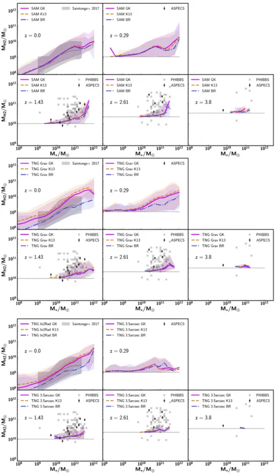
First, we find no significant difference in the predicted average H2 mass of galaxies by the three different H2
partitioning recipes coupled to the SC SAM. When coupled to IllustrisTNG the GK and K13 recipes yield almost identical results. This is in line with the broaderfindings by Diemer et al. (2018). The BR recipe predicts lower H2masses at z<0.3, but
identical H2 masses at higher redshifts. Given the minimal
deviations in the medians between the different H2partitioning
recipes, we will show from now on only predictions by the GK partitioning method in the main body of this paper. Model predictions obtained when adopting the other H2partitioning
recipes are provided in AppendixB.
Importantly, wefind the H2mass of galaxies to increase as a
function of stellar mass for the SC SAM and IllustrisTNG when adopting the“Grav” aperture, independent of redshift. At z<3 we see a decrease in the median H2 mass for galaxies with a
stellar mass larger than 1010Me. This decrease is stronger for the SC SAM than for IllustrisTNG with the“Grav” aperture. This drop in the median represents the contribution from passive galaxies that host little molecular hydrogen, driven by the AGN feedback mechanism. These galaxies have H2masses
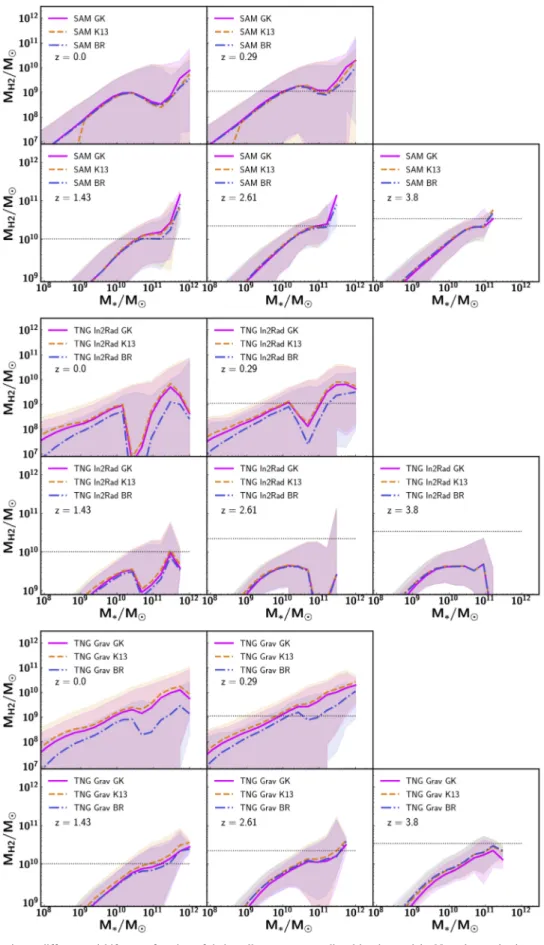
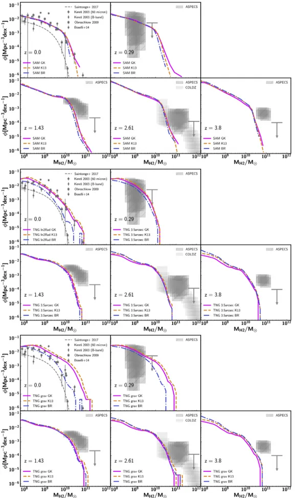
Figure 1.H2mass of galaxies at different redshifts as a function of their stellar mass, as predicted by the models. No galaxy selections were applied to the model
galaxy population. The top two rows correspond to the SC SAM. The middle two rows depict IllustrisTNG when adopting the“3 5” aperture (note that at z=0 we use the“In2Rad” aperture). The bottom two rows show IllustrisTNG when adopting the “Grav” aperture. In all cases, we show results with the three H2partitioning
recipes adopted in this work(GK: solid pink; K13: dashed orange; BR: dotted–dashed blue). The thick lines mark the median of the galaxy population, whereas the shaded regions mark the 2σ scatter of the population. The dotted black horizontal line marks the sensitivity limit of ASPECS.
that are below the sensitivity limit of ASPECS. The upturn at the highest stellar masses corresponds to a low number of central galaxies that are still relatively gas rich.
When adopting the“3 5” aperture for IllustrisTNG we see a different behavior from the “Grav” aperture. At z=0.29 and z=1.43 there is a much stronger drop in the median H2mass
of galaxies at masses larger than 1010Me. This suggests that the bulk of the H2reservoir of the subhalos is outside of the
aperture corresponding to the ASPECS beam at these redshifts. A beam with a diameter of 3 5 at z=0.29 corresponds to a size smaller than two times the stellar half-mass–radius of the galaxies in IllustrisTNG with M*>1010Me (Genel et al.
2018), suggesting that not all the molecular gas close to the
stellar disk is captured. An AGN may furthermore move baryons to larger distances away from the center of the galaxies (outside of the aperture), but this has to be tested further by looking at the resolved H2 properties of galaxies with
IllustrisTNG. Stevens et al. (2018) find a similar drop at
z=0 in the total cold gas mass (HIplus H2) of IllustrisTNG
galaxies at similar stellar masses and also argue that AGN feedback may be responsible for this.
Putting the predicted H2 mass in contrast to the ASPECS
sensitivity limit gives an idea of which galaxies might be missed by ASPECS. At z=0.29 the ASPECS sensitivity limit is below the median of the entire population of galaxies with stellar masses larger than 1010Mefor the SC SAM and IllustrisTNG when adopting the “Grav” aperture. When adopting the “3 5” aperture the situation changes, and only the most H2massive
galaxies are picked up by the ASPECS survey(well above the median). The same conclusions are roughly true at z=1.43. At z=2.61 the ASPECS sensitivity limit is below the median of the galaxy population as predicted by the SAM for galaxies with M*>1011Me. The ASPECS survey is sensitive to the galaxies with the largest H2 masses with stellar masses in the range
1010Me<M*<1011Me. Galaxies with lower stellar masses are excluded by the ASPECS sensitivity limit, according to the predictions by the SC SAM. The ASPECS sensitivity limit at z=2.61 is always above the median predictions from IllustrisTNG, independent of the aperture. At z=3.8 the ASPECS sensitivity limit is always above the median predictions by the models(both the SC SAM and IllustrisTNG). According to the models, ASPECS is only sensitive to galaxies with stellar masses ∼1011Me with the most massive H2 reservoirs (see
Section5for a more in depth discussion on this).
4.1.2. Mocked Results
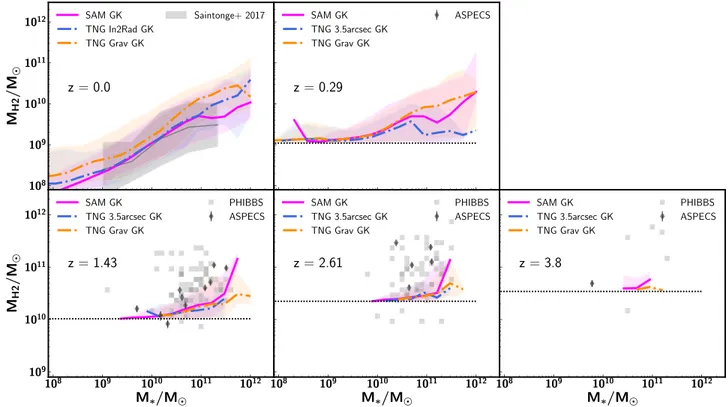
In Figure 2 we again present the H2 mass of galaxies as a
function of their stellar mass at z=0 and at the median redshifts of ASPECS predicted from IllustrisTNG and the SC SAM. Differently from the previous figure, we now take into account the selection functions that characterize the observational data sets we compare to. In particular, in this figure, the predictions are compared to observed H2masses of galaxies from Saintonge et al.
(2017) at z=0, and to the detections from the ASPECS surveys
(all detections with a signal-to-noise ratio higher than 6.4). as well
Figure 2.Predicted and observed H2mass of galaxies at different redshifts as a function of their stellar mass. For the theoretical data, we account for observational
selection effects. The results from SC SAM(solid pink) and from IllustrisTNG are shown by adopting the GK H2partitioning recipe. We show predictions for
IllustrisTNG when adopting the“3 5” (dashed blue) and “Grav” (dotted–dashed orange) apertures (at z=0, the “3 5” aperture is replaced by the “In2Rad” aperture). In thisfigure we assume αCO=3.6 Me/(K km s−1pc2). At z=0 a comparison is done to observational data from Saintonge et al. (2017). To allow for a fair
comparison and remove the contribution by quiescent galaxies, a selection criterion oflog SFR>log SFRMS(M*)-0.4is applied to both the observed and modeled galaxies at z=0, wherelog SFRMS(M*) marks the SFR of galaxies on the main sequence of star formation, following the definition of Speagle et al. (2014). At higher
redshifts model predictions are compared to the detections of ASPECS, as well as the compilation of CO detected galaxies presented as a part of PHIBBS in Tacconi et al.(2018). At these redshifts the ASPECS selection function is applied to the model galaxies (and depicted by the dotted black horizontal line). The solid lines mark
the median of the galaxy population, whereas the shaded regions mark the 2σ scatter of the population. The different models are only partially able to reproduce the ASPECS and PHIBBS detections. We furthermorefind that the ASPECS sensitivity sets a strong cut on the overall galaxy population (compare to Figure1).
as a compilation presented in Tacconi et al.(2018) as a part of the
PHIBBS(IRAM Plateau de Bure HIgh-z Blue Sequence Survey) survey at higher redshifts. At z=0 a selection criterion of
> M
-log SFR log SFRMS( *) 0.4 is applied to both the observed and modeled galaxies, where log SFRMS(M*) marks
the SFR of galaxies on the main sequence of SF at z=0 following the definition of Speagle et al. (2014). At z=0 the respective
main-sequences predicted by the models are in reasonable agreement with the data, see Donnari et al. (2019) and Hahn
et al.(2019). At higher redshifts we only adopt the ASPECS CO
sensitivity-based selection criterion. ASPECS is sensitive to sources with an H2 mass of ~109M at z=0.29 and ∼1010,
2×10¹⁰, and 3×10¹⁰Me, at z≈1.43, 2.61, and 3.8, respectively (see Boogaard et al. 2019; Decarli et al. 2019, and González-López et al. 2019, for more details).28 The PHIBBS survey selected galaxies based on a lower-limit in stellar mass and SFR. Although this selection criterium is different from the ASPECS survey, the galaxies in PHIBBS that have the most massive H2reservoirs would have also been detected as a part
of ASPECS and can therefore be compared to our model predictions.
At z=0 the predictions by the IllustrisTNG model are in general in good agreement with the observations(Diemer et al.
2019 present a more detailed comparison of the H2 mass
properties of galaxies at z=0 between model predictions and observations, accounting for beam/aperture effects and differ-ent selection functions). The typical spread in the relation between H2 mass and stellar mass is smaller for the model
galaxies than the observed galaxies (it is worthwhile to note that the sample size of the observed galaxies is significantly smaller). At higher redshifts, on the other hand, a large fraction of the galaxies detected by ASPECS at z 1.43 are not predicted by either IllustrisTNG (independent of the adopted aperture) or the SC SAM, i.e., the observed galaxies lie outside of the 2σ scatter derived from the models. Similarly, a large fraction of the galaxies that are part of the PHIBBS data compilation also lie outside the 2σ scatter on the predictions by the different models (also at z∼3.8). This suggests that the models predict H2reservoirs as a function of stellar mass that
are not massive enough at z∼1–3.
Note that the median trends predicted from IllustrisTNG and the SC SAM at z=0 are essentially identical at low stellar masses, 1011Me. However, they diverge at larger stellar masses. The H2 masses predicted from IllustrisTNG at
z=0 are a factor ∼2 higher than the SC SAM’s ones above 1011Me, the precise estimate depending on the adopted aperture. At z∼0.29 the H2 scaling relations predicted by
the models when accounting for the ASPECS sensitivity limits begin to differ for galaxies with stellar masses larger than ∼7×10¹⁰M
e. At higher redshifts, the SC SAM and
IllustrisTNG predict similar H2masses for galaxies with stellar
masses less than 1011Me(an artifact of the imposed selection limit), while at larger stellar masses the SAM predicts slightly more massive H2reservoirs atfixed stellar mass. Overall, the
predictions of the SC SAM and IllustrisTNG are surprisingly similar, considering the large number of differences in the underlying modeling approach.
4.2. The Evolution of the H2Mass Function
We show the H2mass function of galaxies as predicted from
IllustrisTNG and the SC SAM for the GK H2 partitioning
recipe in Figure3 (the H2mass functions predicted using the
other H2 partitioning recipes are presented in Appendix B,
where we show that they are very similar). The H2 mass
functions are shown at z=0 and at the median redshifts probed by ASPECS. The theoretical mass functions are derived by accounting for all the galaxies in the full simulation box (∼100 cMpc, solid line). The shaded regions mark the spread in the mass function when calculating it in smaller boxes representing the ASPECS volume, which is further discussed in Section 4.2.1. The mass functions at z=0 are compared to observations taken from Keres et al. (2003), Obreschkow &
Rawlings (2009), Boselli et al. (2014), and Saintonge et al.
(2017, assuming a CO-to-H2 conversion factor of αCO=
3.6 Me/(K km s−1pc2)). The Obreschkow & Rawlings (2009)
and Keres et al.(2003) mass functions are based on the same
data set, only Obreschkow & Rawlings (2009) assumes a
variable CO-to-H2conversion factor as a function of metallicity
(unlike ASPECS) instead of a fixed CO-to-H2 conversion
factor. At higher redshifts we compare the model predictions to the results from ASPECS, as well as the results from the COLDZ survey at z∼2.6 (Pavesi et al.2018; Riechers et al.
2019).
The H2mass function at z=0 predicted by the SC SAM
is in good agreement with the observations (Keres et al.
2003; Boselli et al. 2014; Saintonge et al.2017).29The mass function as predicted from IllustrisTNG when adopting the “In2Rad” aperture (similar to the observed aperture) is also in rough agreement with the observations. When adopting the “Grav” aperture the number densities of the most massive H2
reservoir are instead too high. This difference highlights the importance of properly matching the aperture over which measurements are taken, especially at low redshifts and at the high mass end. Diemer et al. (2019) present a robust
comparison between model predictions from IllustrisTNG and observations at z=0, better accounting for the beam size of the various observations at z=0 than is done in this work.
Both the SC SAM and IllustrisTNG reproduce the the observed H2mass function by ASPECS at z∼0.29
(indepen-dent of the aperture). These are at masses below the knee of the mass function. Indeed, the volume probed by ASPECS at z∼0.29 is rather small, which explains the lack of galaxies detected with H2masses larger than a few times 10
9
Me. For the most massive H2reservoirs at z=0.29, on the other hand,
the two models (and the choice of different apertures) return significantly different results: at fixed number density, the corresponding H2mass differs by a factor offive between the
two IllustrisTNG apertures, with the SC SAM in between. At z>1 the predictions for the H2number densities by the
different models and their respective apertures are very close to each other. On average the SC SAM predicts number densities that are ∼0.2 dex higher. At z=1.43 the models only just 28
Like before, we adopt the same CO excitation conditions and CO-to-H2
conversion factor as ASPECS,αCO=3.6 Me/(K km s−1pc2), and assume a
CO linewidth of 200 km s−1. Note that one of the ASPECS sources in Figure2
has an H2 mass below the dotted line representing the ASPECS selection
function. This galaxy has a CO linewidth narrower than 200 km s−1. Accounting for variations in the CO linewidth heavily complicates the selection function that has to be applied to the IllustrisTNG and SC SAM galaxies. We have thus chosen to limit ourselves to a typical value for main-sequence galaxies of 200 km s−1.
29
The differences between the observational mass functions are driven by field-to-field variance, as these surveys target a relatively small area on the sky or sample, sometimes located in known overdensities.
reproduce the observed H2 mass function around masses of
1010Me, but predict too few galaxies with H2 masses larger
than 3×10¹⁰Me. The predicted H2 number densities at
z=2.61 are in good agreement with COLDZ and ASPECS in the mass range of 1010 MeMH26×10
10
Me. The models do not reproduce ASPECS at higher masses and at higher redshifts, predicting number densities that are too low. We will further quantify how well the models reproduce the observed H2 mass function when taking the surface area into
account in the next subsection.
4.2.1. Field-to-field Variance Effects on the H2Mass Function Since ASPECS only surveys a small area on the sky, field-to-field variance may bias the observed number densities of galaxies toward lower or higher values. In Figure 3 the thick lines represent the H2 mass function that is derived when
calculating the H2mass function based on the entire simulated
volume (∼100 cMpc for TNG100). The shaded areas around the thick lines in Figure 3 quantify the effects of cosmic variance on the H2mass function. The shaded regions mark the
2σ scatter when calculating the H2 mass function in 1000
randomly selected subvolumes corresponding to the actual volume probed by ASPECS at the given redshifts (Table1).30
At z=0.29 the small area probed by ASPECS can lead to large differences in the observed H2mass function. This ranges
from number densities less than 10−6Mpc−3dex−1at the lower end of the 2σ scatter to a few times 10−2 Mpc−3dex−1at the upper end of the 2σ scatter at any H2mass. The galaxies with the
largest predicted H2 reservoirs at z=0.29 (MH2>10 10
Me) will typically be missed by a survey like ASPECS(do not fall in between the 2σ scatter). This is indeed reflected by the lack of constraints on the number density of galaxies with H2masses
more massive than 1010Meby ASPECS.
The volume probed by ASPECS at redshifts z>1 is significantly larger (see Table1), which indeed results in less
scatter in the H2number densities of galaxies due to
field-to-field variance. The 2σ scatter in the power-law component of the mass function is 0.2–0.3 dex for IllustrisTNG and the SC SAM. The scatter quickly increases at H2masses beyond the
knee of the mass functions, ranging from number densities less than 10−6Mpc−3dex−1to number densities a few times higher than inferred based on the entire simulated boxes. The model
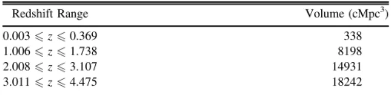
Table 1
The Volume(in Comoving Mpc) Probed by ASPECS in Different Redshift Ranges, after Correcting for the Primary Beam Sensitivity(See Decarli et al.
2019)
Redshift Range Volume(cMpc3)
0.003z0.369 338
1.006z1.738 8198
2.008z3.107 14931
3.011z4.475 18242
Figure 3.Predicted and observed H2mass function of galaxies assumingαCO=3.6 Me/(K km s−1pc2) at z=0 and the redshifts probed by ASPECS. Model
predictions are shown for the SC SAM(solid pink) and IllustrisTNG (“3 5” aperture: dashed blue; “Grav” aperture: dashed–dotted orange), both models adopting the GK H2partitioning recipe. In thisfigure the thick lines mark the mass function based on the entire simulated box (∼100 cMpc on a side for IllustrisTNG, ∼142 cMpc
on a side for the SC SAM). The colored shaded regions mark the 2σ scatter when calculating the H2mass function in 1000 randomly selected cones that capture a
volume corresponding to the volume probed by ASPECS at the given redshifts(Table1). At z=0 the model predictions are compared to observations from Keres
et al. (2003), Obreschkow & Rawlings (2009), Boselli et al. (2014), and Saintonge et al. (2017). At higher redshifts the model predictions are compared to
observations from the ASPECS and COLDZ(Riechers et al.2019) surveys.
30
Note that these correspond to cylinders covering an area of 4.6 arcmin squared. These cylinders go through a single snapshot that represents the median redshift of the different ASPECS bins and not a continuous lightcone. We loop through the periodic box multiple times to reach the same volume as probed by ASPECS. In doing so we ensure not to count the same galaxy twice. We will present lightcones based on IllustrisTNG and the SC SAM in future works.
galaxies that host the largest H2reservoirs in the full modeled
boxes are typically not recovered when focusing on small volumes similar to the volume probed by ASPECS.
We can make a fairer comparison between the predictions by the theoretical models and ASPECS by accounting for the small volume probed by ASPECS. Figure3shows that at z>1 the observed number density of galaxies with MH2>1011Me
is outside of the 2σ scatter of the model predictions by both IllustrisTNG(for both apertures) and the SC SAM. The number densities of galaxies with lower H2masses are within the 2σ
scatter of both models. Summarizing, both IllustrisTNG and the SC SAM do not predict enough H2rich galaxies(with masses
larger than 1011Me) in the redshift range 1.4z3.8. This is in line with ourfindings in Section4.1that both IllustrisTNG and the SC SAM predict H2masses within this redshift range
that are typically too low for their stellar masses compared to the observations from ASPECS and PHIBBS.
4.3. The H2Cosmic Density
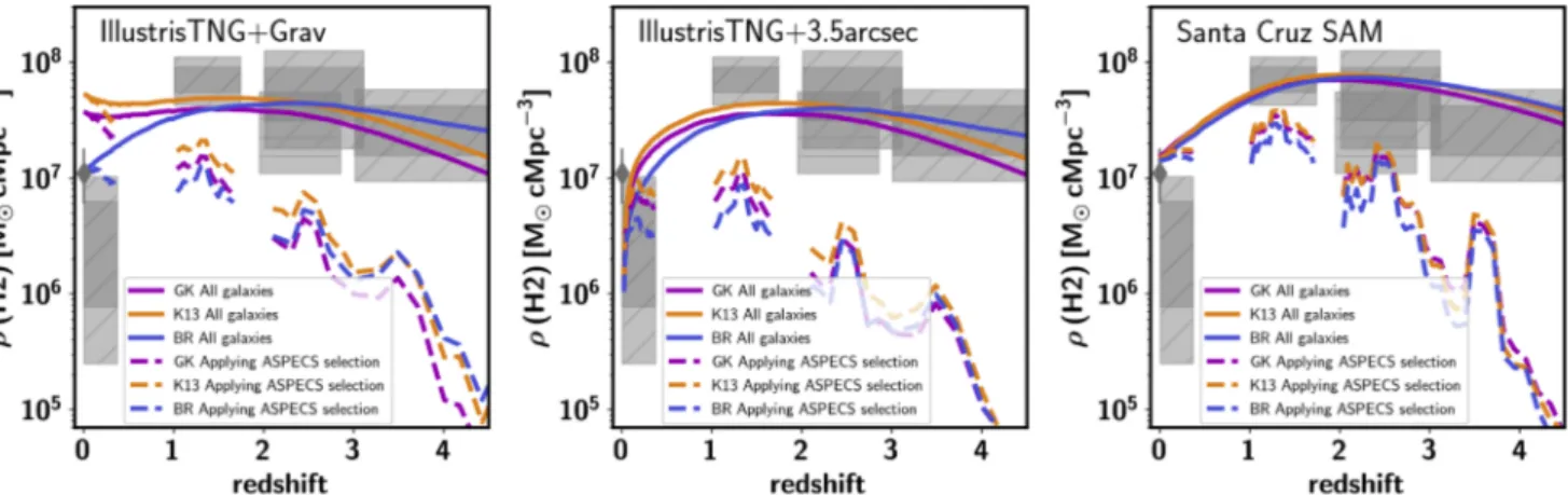
We present the evolution of the cosmic density of H2within
galaxies predicted by the SC SAM and IllustrisTNG when adopting the GK partitioning recipe in Figure4(predictions for
the other partitioning recipes are presented in Appendix B).
The solid lines correspond to the cosmic density derived based on all the galaxies in the entire simulated volume. The dashed lines correspond to a scenario where we only include galaxies with H2masses larger than the detection limit of ASPECS. The
shaded region marks the H2cosmic density calculated in a box
with a volume that corresponds to the volume probed by ASPECS at the appropriate redshift. This is further explained in Section 4.3.1. The model predictions are compared to z=0 observations taken from Keres et al.(2003) and Obreschkow &
Rawlings(2009), as well as the observations from the ASPECS
and COLDZ(Riechers et al.2019) surveys at higher redshifts.
The H2 cosmic density predicted from IllustrisTNG when
adopting the “Grav” aperture gradually increases until z=1.5 after which it stays roughly constant until z=0. At z∼1, accounting for the ASPECS sensitivity limits can lead to a reduction in the H2 cosmic density of a factor of three. The
reduction is one order of magnitude at z∼2 and further increases toward higher redshifts. The H2 cosmic density
predicted from IllustrisTNG when adopting the “3 5” aperture increases until z∼2 and stays roughly constant until z=1. The H2cosmic density rapidly drops at z<1 by almost an order of
magnitude until z=0. The difference between the low-redshift evolution predicted when adopting the “Grav” aperture versus the “3 5” aperture (especially at z<0.5) indicates that the “3 5” aperture misses a significant fraction of the H2associated
with the galaxy. The decrease in H2 cosmic density when
accounting for the ASPECS sensitivity limits is similar for the “3 5” aperture as the “Grav” aperture. The decrease is approximately a factor of three at z=1, approximately an order of magnitude at z=2, and this increases toward higher redshifts.
The H2cosmic density as predicted by the SC SAM when
including all galaxies increases until z∼2, after which it gradually decreases by a factor of ∼4 until z=0. Similar to IllustrisTNG, accounting for the ASPECS sensitivity limits results in a drop in the H2cosmic density of a factor of∼3 at
z=1 and approximately an order of magnitude at z>2. On average, the SC SAM predicts H2 cosmic densities at z>1
that are 1.5–2 times higher than predicted from IllustrisTNG
(note that the SC SAM also predicts higher number densities for H2-rich galaxies at these redshifts).
The difference between the total cosmic density (i.e., including the contribution from all galaxies in the simulated volume) and the H2cosmic density after applying the ASPECS
sensitivity limit highlights the importance of properly account-ing for selection effects when comparaccount-ing model predictions to observations. Too often, comparisons are only carried out at face value ignoring these effects, creating a false impression. In this analysis wefind that, when taking the ASPECS sensitivity limits into account, the cosmic densities predicted by the models are well below the observations at z>1, independent of the adopted model, H2partition recipe, and aperture. In the
next subsection we will additionally take the effects of cosmic variance into account, in order to better quantify the (dis) agreement between ASPECS and the model predictions.
4.3.1. Field-to-field Variance Effects on the H2Cosmic Density To understand the effects of field-to-field variance on the results from the ASPECS survey we also calculate the H2
cosmic density in boxes representing the ASPECS volume. The shaded regions in Figure4mark the 0th and 100th percentile, 2σ and 1σ scatter when calculating the H2 cosmic density in
1000 randomly selected cones through the simulated volume that correspond to the volume probed by ASPECS (as described in Section 4.2.1, in this case also accounting for the ASPECS sensitivity limit).31
At z<0.3 field-to-field variance can lead to large variations already(multiple orders of magnitude within the 2σ scatter) in the derived H2 cosmic density of the universe, both for
IllustrisTNG and the SC SAM. At higher redshifts the volume probed by ASPECS is larger and indeed the scatter in the H2
cosmic density is smaller than at z<0.3.
The ASPECS observations at z∼1.43 are reproduced by a small fraction of the realizations predicted from IllustrisTNG (independent of the aperture), corresponding to the area above the 2σ scatter (i.e., only up to 2.5% of the realizations drawn from IllustrisTNG reproduce the ASPECS observations). The observations at z∼1.43 are reproduced by a larger fraction of the realizations drawn from the SC SAM, covering the area between the 1σ and 2σ scatter and above.
At 2<z<3 all the realizations drawn from IllustrisTNG (independent of the chosen aperture) predict H2 cosmic
densities lower than the ASPECS observations. At z>3 only a small fraction of the realizations reproduce the ASPECS observations when adopting the “Grav” aperture, corresp-onding to the area between the 2σ scatter and 100th percentile. The SC SAM predicts slightly higher cosmic densities on average, although still in tension with the ASPECS observa-tions at z>2. Both IllustrisTNG and the SC SAM reproduce the observations taken from COLDZ in a subset of the realizations.
It is important to realize that a model is not necessarily ruled out if not all of the realizations agree with the ASPECS results. The fraction of realizations that agrees with the ASPECS results gives a feeling for the likelihood of a model being realistic. If only a small fraction (or none) of the realizations reproduces the ASPECS observations, this suggests that the 31
At some redshifts, for example, z>3.5, the shaded area corresponding to the 1σ scatter appears to be missing. At these redshifts the 1σ area falls below the minimum H2density depicted in thefigure and is therefore not shown.
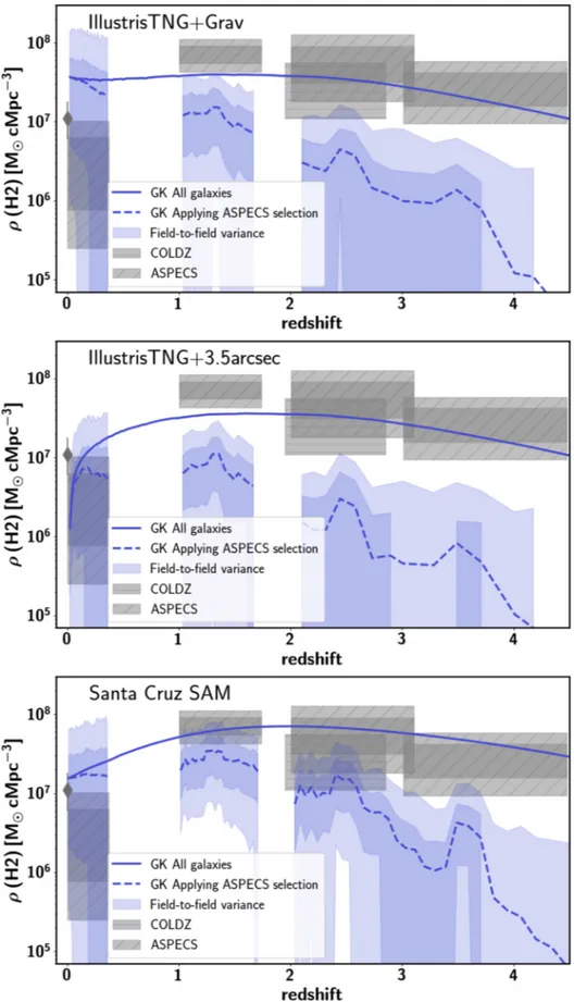
Figure 4.Predicted and observed H2cosmic density assumingαCO=3.6 Me/(K km s−1pc2) as a function of redshift predicted from IllustrisTNG (“Grav” aperture,
top;“3 5” aperture, center), and the SC SAM (bottom), adopting the GK H2partitioning recipe. Solid lines correspond to the cosmic H2density based on all the
galaxies in the entire simulated volume. Dashed lines correspond to the cosmic H2density when applying the ASPECS selection function. Shaded regions mark the 2σ
and 1σ scatter when calculating the H2cosmic density in 1000 randomly selected cones that capture a volume representing the ASPECS survey. Observations are from
model is very likely to be invalid(modulo the assumptions with regards to the interpretation of the observations). We will come back to this in the discussion.
5. Discussion
5.1. Not Enough H2in Galaxy Simulations?
One of the main results of this paper is that, when a CO-to-H2
conversion factor αCO=3.6 Me/(K km s−1pc2) is assumed,
both IllustrisTNG and the SC SAM predict H2masses that are
too low at a given stellar mass for galaxies at z>1 (Figure2),
do not predict enough H2-rich galaxies (with H2masses larger
than 3×10¹⁰Me; Figure3), and predict cosmic densities that
are in tension with the ASPECS results after taking the ASPECS sensitivity limits and field-to-field variance into account (Figure 4). There are multiple choices that have to be made
(both from the theoretical and observational side) that will affect this conclusion. In the remainder of this subsection we discuss the main ones.
5.1.1. The Strength of the UV Radiation Field Impinging on Molecular Clouds
One of the theoretical challenges when calculating the H2
content of galaxies is accounting for the impinging UV radiation field. Diemer et al. (2018) explored multiple
approaches, by increasing and decreasing the UV radiation field when calculating the H2mass of cells in the IllustrisTNG
simulation. The authors found differences in the predicted H2
masses within a factor of 3 for the most extreme scenarios tested in their work (ranging from 1/10 to 10 times their fiducial UV radiation field, where a stronger UV radiation field results in lower H2masses), with differences away from their
fiducial model up to a factor of 1.5–2. Although a systematic decrease in the UV radiationfield could help to reproduce the cosmic density of H2, it would go at the cost of reproducing the
H2 mass of galaxies and their mass function at z=0.
Furthermore, a factor of 1.5–2 higher H2 masses would still
not be enough to overcome the tension between model predictions and observations at z>2. In the context of the SC SAM, SPT15 explored two different approaches to calculate the strength of the UV radiation field and found minimal changes in the predicted H2 mass of galaxies with a
z=0 halo mass larger than 1011Me.
5.1.2. The CO-to-H2Conversion Factor and CO Excitation Conditions
One of the major observational uncertainties that could alleviate the tension between model predictions and the ASPECS results is the CO-to-H2 conversion factor. The
ASPECS survey adopts a conversion factor ofαCO=3.6 Me/
(K km s−1pc2) for all CO detections. We first explore what
values for the CO-to-H2conversion factor would be necessary
to bring the model predictions into agreement with the observations. Changing the assumption for αCO has two
immediate consequences. First, it changes the value of the observed H2mass. Second, it changes the H2mass limit below
which galaxies are not detected (because observations have a CO rather than an H2 detection limit). Additionally, it is
important to better constrain the ratio between the CO J=1–0 and higher order rotational transitions of CO (J=2–1 to J=4–3 in the ASPECS survey). This ratio is currently
assumed to be afixed number, but has been shown to vary by a factor of a few from Milky Way–type galaxies to ULIRGS.
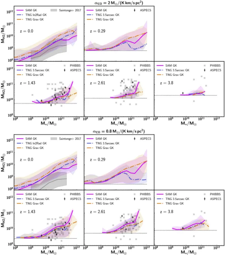
We show the H2 mass of galaxies as a function of stellar
mass when varying the CO-to-H2conversion factor in Figure5.
The model predictions at z=1.43 are in significantly better agreement with the ASPECS detections when adopting αCO=2.0 Me/(K km s−1pc2) than the standard value of
αCO=3.6 Me/(K km s−1pc
2), although there is still a
sig-nificant number of galaxies detected as part of the PHIBBS survey with H2masses outside of the 2σ scatter of the models.
More than half of the ASPECS detections at z=2.61 fall outside of the 2σ scatter of the model predictions when adopting αCO=2.0 Me/(K km s−1pc2). When assuming
αCO=0.8 Me/(K km s−1pc2), the model predictions are in
good agreement with the ASPECS detections at z=1.43 and z=2.61 (although there are still a number of PHIBBS detections not reproduced by the models). We do note that the better match at z>1 comes at the cost of predicting H2
masses that are too massive at z=0.
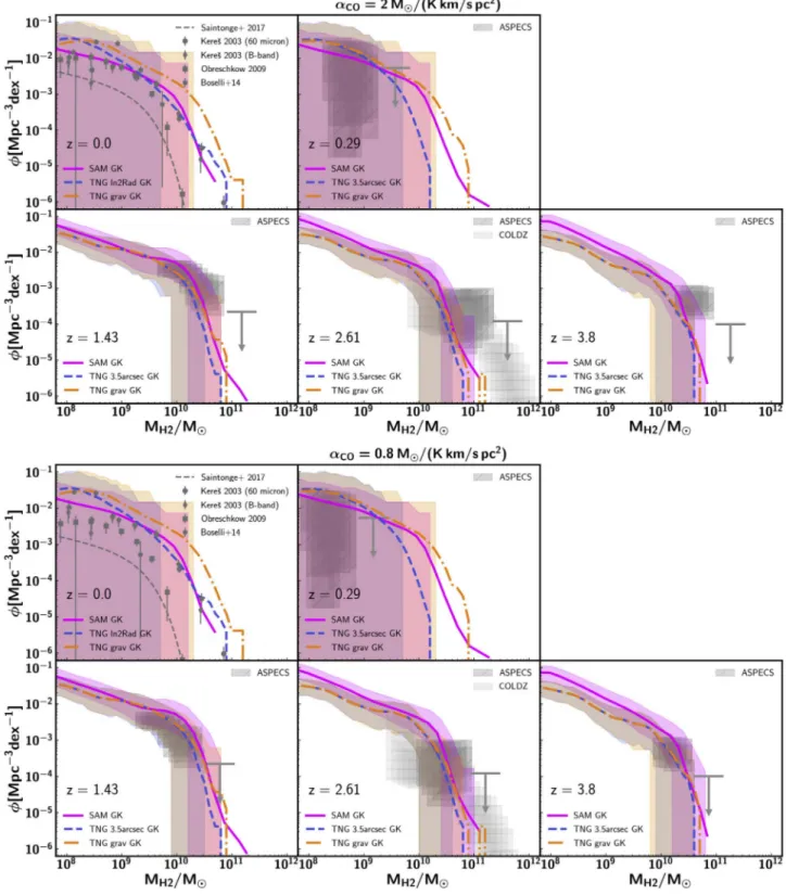
We present the observed and predicted H2mass function of
galaxies when assuming different values forαCOin Figure 6.
Wefind that when adopting αCO=2.0 Me/(K km s−1pc 2) the
models reproduce the observed ASPECS H2mass function of
galaxies over cosmic time (after accounting for cosmic variance, Figure 6 top panels versus Figure 3). The number
density of massive galaxies(larger than 1011Me) detected as a part of the COLDZ survey are still not reproduced by the models(i.e., the observed number densities are outside of the 2σ scatter of the model predictions). A CO-to-H2conversion
factor of αCO=0.8 Me/(K km s−1pc2) brings the model
predictions for the H2 mass functions from IllustrisTNG and
the SC SAM into excellent agreement with the results from ASPECS at 1z4 (Figure5, lower panels) and yields the best agreement with the COLDZ results.
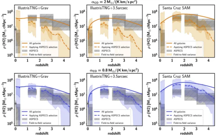
When adopting αCO=2.0 Me/(K km s−1pc2), both models
return a larger fraction of volume realizations that are consistent with the ASPECS and COLDZ H2cosmic densities at all redshifts
(Figure7, top panels). The ASPECS observations fall well within the 2σ scatter of the predictions by the SC SAM. The observations fall in the area between the 2σ scatter and 100th percentile of the predictions by IllustrisTNG when adopting an aperture corresp-onding to 3 5. When adopting αCO=0.8 Me/(K km s−1pc2),
the ASPECS results overlap the predictions by both models(and both apertures for IllustrisTNG). For this scenario, only the lower 32% of all the realizations predicted by the SC SAM matches the observations. Similar conclusions hold when comparing the model predictions to the COLDZ survey. We do note that reproducing the ASPECS results at z>1 by varying the CO-to-H2conversion factor for all galaxies comes at the cost of
predicting H2masses for galaxies at z=0 that are too massive.
Summarizing, the ASPECS survey would need to adopt a conversion factor of aCO~0.8M (K km s-1pc2) for all observed galaxies at z>0 for the models to better reproduce the observed H2 mass function and the H2 cosmic density.
The CO-to-H2 conversion factor adopted by ASPECS of
αCO=3.6 Me/(K km s−1pc
2) is motivated for main-sequence
galaxies based on dynamical masses (Daddi et al. 2010), CO
line spectral energy distribution (SED) fitting (Daddi et al.
2015) and solar metallicity z>1 main-sequence galaxies
(Genzel et al. 2012). Nevertheless, conversion factors of
a ~2M K km s- pc
CO ( 1 2) have been found for