The Italian banking industry: efficiency, market power, role in the local economies

(1)

UNIVERSITA’ DEGLI STUDI DI SALERNO

Dipartimento di Scienze Economiche e Statistiche

Dottorato di ricerca in Economia del Settore Pubblico

VIII ciclo (nuova serie)

Tesi di Dottorato

in

The Italian banking industry:

efficiency, market power, role in the local

economies

Coordinatore:

Prof. Sergio Pietro DESTEFANIS

Relatore:

Prof. Paolo COCCORESE

Candidato:

Dott. Alfonso PELLECCHIA

(2)

(3)

3

TABLE OF CONTENTS

ACKNOWLEDGEMENTS 4

INTRODUCTION 5

CHAPTER ONE - Estimating Scale and Scope Economies in Banking: Evidence from a Multi-output Symmetric Generalized McFadden Cost Function

1.1 Introduction 7

1.2 A brief review of the literature 8

1.3 Methodology 11

1.4 Data and definition of the variables 15

1.5 Estimation results 17

1.6 Conclusion 21

CHAPTER TWO - Testing the “Quiet Life” Hypothesis in the Italian Banking Industry

2.1 Introduction 22

2.2 Market power, efficiency, and their relationship: a review of the banking literature

24 2.3 Estimation of cost efficiency and market power 29

2.4 Testing the “quiet life” hypothesis 31

2.5 Data and variables 34

2.7 Conclusions 48

CHAPTER THREE - Local Economic Growth and the Role of Banks

3.1 Introduction 50

3.2 Banking market structure, financial development and growth: review of the literature

51

3.3 The econometric model 56

3.4 Estimating efficiency and market power 64

3.5 Data 67

3.7 Summary and conclusions 82

(4)

4

ACKNOWLEDGEMENTS

I am deeply grateful to my advisor, Prof. Paolo Coccorese, for his guidance, help and encouragement.

I would also like to thank the coordinator of the Ph.D. program, Prof. Sergio Pietro Destefanis, for his support and suggestions.

(5)

5

INTRODUCTION

In the last twenty years the banking sector of many countries has undergone a period of consolidation and restructuring. This has raised concerns about the welfare implications of larger credit institutions, given that the banking industry is vital for the whole economic system.

From a theoretical point of view, one should expect two “direct” effects from these structural transformations. First of all, consolidation may allow banks to achieve a higher level of efficiency thanks to the exploitation of scale and scope economies. Secondly, mergers and acquisitions among credit institutions could lead to an increase in local market concentration and thus, as maintained by the Structure-Conduct Performance (SCP) paradigm, to an increase in banks’ market power.

In turn, market power in banking is the channel through which the consolidation process could have some “indirect effects” on other economic phenomena. Indeed, as shown by recent empirical works, the degree of competition in banking markets is a key explanatory variable of banks’ X-efficiency, as well as credit availability for small firms, relationship banking, economic growth and financial stability.

In this dissertation we empirically explore some of the consequences of the consolidation process, focusing on the Italian banking industry. More precisely,

Chapter One studies the effect on banks’ cost efficiency. Starting from a Multi-output

Symmetric Generalized McFadden cost function, we estimate a system of factor demand equations in order to assess the degree of scale and scope economies of Italian banks in the period 1992-2007. We find evidence of slight economies of scale and significant economies of scope. Our main conclusion is that the efficiency gains coming from merger and acquisition operations could be an explanation of the consolidation process; at the same time, they could translate into beneficial effects for consumers and firms, provided that they are not offset by an increased market power.

In the following chapters we turn to the possible indirect effects of banking consolidation. The focus of Chapter Two is on the impact of banks’ monopoly power on their X-efficiency. Particularly, we test the so-called “quite life” hypothesis (QLH), according to which firms with market power are less efficient. Using data for the period 1992-2007, we apply a two-step procedure. First, we estimate bank-level cost efficiency scores and Lerner indices. Then we use the estimated market power measures, as well

(6)

6

as a vector of control variables, to explain cost efficiency. Unlike the existing literature on the subject, to this end we employ a logistic regression that, in our opinion, is better suited to model cost efficiency scores. Our empirical evidence supports the QLH, although the impact of market power on efficiency is not particularly remarkable in magnitude.

Finally, in Chapter Three we assess the impact of banks’ market power, and other structural variables characterizing banking markets, on local economic growth. Using a dataset on the Italian provinces for the period 1999-2006, as well as banks’ balance sheets data, we estimate a dynamic panel data model, also taking into account the possible spatial dependence among observations. This is a novelty in the empirical literature on the finance-growth nexus. Moreover, the use of data on local economies, allows us to control more easily for heterogeneity. Our results show a positive and statistically significant relationship between banks’ market power and economic growth, thus supporting the view according to which competition in banking can be detrimental to growth because it tends to reduce credit availability for informationally opaque firms. This evidence can have important implications on the Italian economy, where the presence of small (usually more opaque) firms is quite relevant. Besides, when spatial interactions are accounted for, the impact of local financial development disappears, and provincial growth is positively linked to how fast contiguous provinces grow.

Although the three chapters, as explained above, are to some extent linked, they have been organized and written as self-contained works.

(7)

7

CHAPTER ONE

Estimating Scale and Scope Economies in Banking: Evidence

from a Multi-output Symmetric Generalized McFadden Cost

Function

1.1 Introduction

The estimation of scale and scope economies in banking has a long tradition in applied economics and the methodology has evolved according to the introduction of new functional forms. Not all of these, however, are well suited for assessing cost economies and, in particular, economies of scope.

The most used flexible functional form,1 the translog cost function (TCF),2 suffers from two weaknesses. On one hand, it often violates the theoretical property of concavity in prices. Although global concavity can be imposed, this destroys the flexibility of the TCF.3 On the other hand, it does not admit zero values of outputs, since all variables enter in logarithmic form. Then it is not possible to assess economies of scope. Several solutions have been proposed to deal with this undesirable characteristic of the TCL, none of which is completely satisfactory (Pulley and Humphrey, 1993).

The quadratic cost function, originally proposed by Lau (1974), admits zero output values but it cannot be restricted parametrically in order to impose homogeneity and/or concavity in input prices without sacrificing its flexibility. The same applies for the Generalized-CES-Quadratic cost function introduced by Roller (1990).

Caves et al. (1980) proposed to use the Box-Cox transformation of the outputs in the translog model in order to accommodate zero values. However, empirical applications using this cost function show that the parameter of the transformation is nearly zero, so that the estimated Generalized translog cost function is a close approximation to the

1

For the definition of flexibility, see Diewert (1974).

2

The translog functional form has been introduced by Christensen et al. (1973).

3

See Diewert and Wales (1987). Concavity can also be imposed locally as showed by Ryan and Wales (2000). Using Berndt and Khaled (1979) dataset (which consists of 25 observations), they find that

(8)

8

translog form. Conversely, the Symmetric Generalized McFadden cost function, introduced by Diewert and Wales (1987) and extended to the multi-output framework by Kumbhakar (1994), admits zero values for outputs and is globally concave in input prices.4

In this paper we assess scale and scope economies in the Italian banking industry over the period 1992-2007. We estimate a system of factor demand equations derived from a Multi-product Symmetric Generalized McFadden (MSGM) cost function.5 Using a panel of banks, we are also able to control for technical change.

Reliable estimates cost economies in banking are very relevant from a policy point of view, due to the consolidation process that has taken place in Italy (as in many other countries) in the last twenty years.6 Indeed, an effect (and at the same time a cause) of the consolidation could be the exploitation of scale and scope economies by larger and more diversified institutions and then lower interest rates on loans. If this is the case, to the extent to which those effects are not offset by an increased market power of banks, we should expect welfare gains from the ongoing consolidation in the banking industry. The paper is organized as follows. Section 1.2 offers a brief review of the empirical literature on banking costs. Section 1.3 discusses the properties of the MSGM and the related measures of economies of scale, economies of scope and technical change. The dataset is described in Section 1.4, while in Section 1.5 results are presented and interpreted. Finally, Section 1.6 draws some conclusions.

1.2 A brief review of the literature

Early studies on costs in the banking industry date back to the mid-1950s. An excellent review on this first stage of research can be found in Gilbert (1984). Since imposing curvature conditions locally results in concavity at all points. However, this is less likely to happen for larger dataset.

4

Anyway, concavity can be imposed through a simple reparametrization, without destroying the flexibility of the cost function.

5

To our best knowledge no previous attempts have been made to assess cost economies in banking using a MSGM cost function. Barnett et al. (1995) employ this functional form to model banks’ technology but in a macroeconomic framework.

6

To give an idea, in Italy the number of banks reduced from 922 in 1998 to 806 in 2007, while in the same period the assets of the whole banking system increased from 1936.71 to 3871.32 billions euro (Bank of Italy data).

(9)

9

then, the methodology has quickly evolved, stimulated by the introduction of new functional forms.

One of the first studies employing a flexible functional form, namely the translog, is Benston et al. (1982). They use an aggregated measure of deposits and loans as output to estimate economies of scale for U.S. banks over the period 1975-1978. However, if one uses a single output specification, the finding of economies of scale could actually be due to the presence of economies of scope (Mester, 1987). Moreover, Kim M. (1986) tests the existence of a consistent output aggregate for a sample of Israeli banks, concluding that a composite measure of output is not able to adequately represent the banking technology.

Murray and White (1983) employ a translog cost function with multiple outputs. Using cross-section data on 61 credit institutions in British Columbia for the period 1976-1977, they find evidence of economies of scale for all banks in the sample, with a weak inverse relationship between returns to scale and asset size. Moreover, they find strong evidence of cost complementaries between mortgage lending and consumer lending.

Another study using a multi-product translog specification is that of Gilligan et al. (1984). The authors use the same data as Benston et al. (1982) but don't find evidence of economies of scale. However, like Murray and White (1983), they conclude that economies of scope exist, although they define bank output quite differently and use data with a lower level of disaggregation.

Using the parameter estimates of Murray and White, Kim H.Y. (1986) performs a richer analysis of credit institution in British Columbia. He observes that the authors omit to consider product-specific economies of scale that arise from the production of a specific subset of products. Moreover, they estimate cost complementaries, which are a sufficient but not necessary condition for economies of scope. Kim finds almost constant return to scale for mortgage lending and investments, diseconomies of scale for consumer lending, and strong evidence of both overall and product-specific economies of scope.

Cebenoyan (1988) estimates only economies of scale of U.S. banks for the period 1980-1983. Running different regressions for each year and separately for unit and

(10)

10

multi-branching banks, he finds evidence of slight diseconomies of scale except for 1983.

Using data on 149 Saving and Loans institutions operating in California in 1982, Mester (1987) finds no evidence of both economies of scale and scope, but evidence of strong substitutability between capital and labour and between labour and demand deposits. Moreover, she shows that there are no cost advantages for institutions with larger branch networks.

One of the drawbacks of the translog cost function is that it is not defined at value zero for one or more outputs. An alternative is to employ the Generalized translog cost function. Lawrence (1989) adopts this type of flexible form to estimate economies of scale and scope for a sample of U.S. banks. Using data for the period 1979-1982, he cannot reject the hypothesis that there are no economies of scope.

None of the studies discussed so far control for technical change, being based on cross-section data. A study taking into account technical change is due to Hunter and Timme (1986). Using a balanced panel of U.S. bank for the period 1972-82 and a single-output translog specification, they find that, on average, costs reduced by 15 per cent during the sample period because of technical progress. Particularly, these benefits were obtained to a larger extent by banks with more branches or higher levels of output. Another flexible functional form used in the banking literature is the Fourier cost function.7 For example, Mitchell and Onvural (1996) use it to estimate scale and scope economies on a sample of about 300 U.S. banks for the years 1986 and 1990. They do not find evidence of neither economies of scale nor economies of scope.

More recent studies, based on models that take into account banks’ risk preferences and financial capital, find scale economies for largest banks.8

Although the cost structure of European banks has not been so extensively studied as that of the U.S., the empirical research available is quite mixed. For example, Glass and McKillop (1992) use data from a single Irish bank to estimate economies of scale, economies of scope and the rate of technical change for the period 1972-1990. They find overall diseconomies of scale, but product-specific economies for lending.

7

This functional form, introduced by Gallant (1981), combines a translog form with a truncated non- parametric Fourier series.

8

(11)

11

Estimation results suggest the presence of diseconomies of scope. As regarding technical change, they estimate an average annual rate of about 5%, except for the period 1975-1977.

A more comprehensive study on technical change is that of Altunbas et al. (1999). The authors estimate a Fourier cost function in a stochastic frontier framework. Using a large panel of European banks for the period 1989-1996, they find that the reduction in costs due to technical change varied between 2.8% and 3.6% over the sample period, with larger banks gaining more benefits.

Regarding single country studies, Zardkoohi and Kolari (1994) use data on 615 branch offices of Finnish bank in 1988 to estimate a translog cost model. The findings are that larger branches operate more efficiently, especially if they belong to banks with large branch networks. Conversely, they do not find evidence of economies of scope.

Two other studies on European country are Dietsch (1993), who finds scale economies for French banks, and Rime and Stiroh (2003), who reports economies of scale for small-medium banks and weak evidence of economies of scope in Switzerland.

For the Italian banking system, the works of Cossutta et al. (1988), Baldini and Landi (1990) and Conigliani et al. (1991) show the presence of economies of scale but not of economies of scope. The last finding, however, has not been confirmed by more recent studies. Cavallo and Rossi (2001) estimate economies of scale and scope on a panel data of banks of six European countries. For Italy, they conclude that global economies of scale exist especially for small banks. Product specific economies of scale are found for deposits and financial investments, and there is evidence of economies of scope both global and product specific.

1.3 Methodology

In order to estimate scale and scope economies in the Italian banking industry, we employ a MSGM cost function. This functional form has been introduced by Kumbhakar (1994), building on the single output specification of Diewert and Wales

(12)

12

(1987), who in turn generalized the McFadden (1978) cost function. It has been used, among others, by Asai (2006), Stewart (2009), and Ivaldi and McCullough (2008).9

The MSGM with M outputs and N inputs can be written as:

( )

1 1 1 1 1 1 2 1 1 1 1 1 1 M N N M N M k k i i ii i k k ik i k k i i k i k N N M M N M t i i i i jk j k tt i i k k i i j k i k C g W Q bW b W Q a W Q t a t W W d Q Q a t W Q β β α λ δ β = = = = = = = = = = = = ⎛ ⎞ = + +_⎜ _⎟ + ⎝ ⎠ ⎛ ⎞ ⎛ ⎞ +_⎜ _⎟ + _⎜ _⎟ ⎝ ⎠ ⎝ ⎠

∑

∑∑

∑

∑∑

∑

(1)

where Q is the k-th output, _k W is the i-th input, t is a time trend,_i 10 and d_jk =d_kj. The scalar functiong W

( )

is defined as:

( )

2 W ' SW g W ' W θ = (2)

where W is the N x 1 vector of inputs, S is an N x N negative semidefinite matrix of parameters, and θ is an N x 1 vector of non-negative constants not all zero.

In order to identify the parameters some restrictions are needed. Firstly, we must have SP* = for some vector 0 P of strictly positive prices. If * P is chosen to be the * unit vector, this implies the set of restrictions

1 0 N ij j s = =

∑

for i=1,...,N. Secondly, setting

i i i i Xi

θ α= =λ δ= = , where X is the sample mean of the i-th input quantity, one needs _i to normalize to unity one of the β_k parameters.11 In spite of these restrictions, there are still enough free parameters for the cost function to be flexible.12

9

The single output specification has been employed, for example, by Kumbhakar (1990), Rask (1995) and Nemoto and Goto (2004).

10

The terms involving t account for technical progress.

11

Alternatively, one can set

1 1 M k k β = =

∑

. 12

See Kumbhakar (1994) for details. Moreover, the MSGM could be made even more flexible – in the sense that the number of free parameters is larger than those necessary to ensure flexibility - setting

i Xi

θ = and estimating separately the α , _i λ and _i δ parameters after normalizing to unity _i a_t, a_tt and one of the d_jk parameters.

(13)

13

Regarding the theoretical properties that a cost function should satisfy, the MSGM is linear homogeneous in prices by construction and, as shown by Diewert and Wales (1987), the negative semidefiniteness of the S matrix ensures the global concavity in prices. If the estimated S is not negative semidefinite, one can easily impose it through the reparametrization S= −HH ', where H is an N x N lower triangular matrix, while at the same time maintaining flexibility.13

By the Shephard’s lemma, X_i = ∂ ∂ . Then, starting from (1) we can write the C W_i input demand system as:

( )

(

)

1 1 2 1 1 1 1 1 M M i k k i ii k k k k i M M M M ik k t i i jk j k tt i k k k j k k g W X Q b b Q W a Q t a t d Q Q a t Q , i ,...,N β β α λ δ β = = = = = = ∂ = + + + ∂ + + + =

∑

∑∑

∑

(3) where

( )

(

)

2 2 i i i g W S W W ' SW W ' W ' W θ θ θ ⎡ ⎤ ∂ =⎢ − ⎥ ∂ _⎢_⎣ _⎥_⎦ (4)

and S( )i is the i-th row of the S matrix. Adding a random error u to each equation, and _i assuming that E u

( )

=0 and E uu'

( )

=Σ , where u=

[

u₁ … u '_N

]

, one gets a system of seemingly unrelated regressions that can be estimated by either the nonlinear and iterative version of the Zellner (1962) ’s method or by maximum likelihood.

With the estimated parameters at hand, and following Baumol et al. (1982), the degree of scale economies is measured by:

1 1 1 M M k k k k k C ESC C Q Q η = = = = ∂ ∂

∑

(5) 13

(14)

14

where η_k is the elasticity of the cost function with respect to the k-th output. ESC is the generalization of the conventional measure of scale economies to multi-product firms, assuming that all outputs proportionally change. Returns to scale are increasing, constant or decreasing according to whether ESC is, greater than, equal to, or less than 1, respectively. For the MSGM cost function (1) we have:

( )

(

)

1 1 2 1 1 1 2 1 N N k k ii i ik i i i k N M N i i jk j tt i i k i j i C g W b W a W t Q W d Q a t W , k ,...,M β β λ δ β = = = = = ∂ = + + + ∂ ⎛ ⎞ ₊ ⎛ ⎞ ₌ ⎜ ⎟ ⎜ ⎟ ⎝ ⎠ ⎝ ⎠

∑

(6)

Economies of scope come from the joint production of several outputs. They are defined as (Bailey and Friedlaender, 1982):

(

)

1 0 0 0 0 M k k C ,..., ,Q , ,..., C ESCP C = − =

∑

(7)

Thus, ESCP measures the relative variation in costs due to the combined production of the M outputs. There exist economies of scope if ESCP>0; indeed, if this is the case, the cost of producing the outputs separately is larger than the cost of producing them jointly, so the numerator is positive. By the same reasoning, if

0

ESCP< , there exist diseconomies of scope. Finally, if the outputs are disjoint in the production process, ESCP=0.

The rate of technical change is given by (minus) the growth rate of costs with respect to time, that is:

C t RTC

C

∂ ∂

= − (8)

If this quantity is positive, costs reduce over time at rate RTC thanks to technical change. For the MSGM cost function (1):

(15)

15 1 1 1 1 1 2 N M N N M ik i k t i i tt i i k k i k i i k C a W Q a W a t W Q t = = = α = δ = β ∂ ₌ ₊ ₊ ⎛ ⎞ ⎜ ⎟ ∂

∑∑

∑

_⎝

∑

_⎠

∑

(9)

To better characterize the production process of Italian banks, we also estimate price elasticities of inputs. By definition, the elasticity of input i with respect to the price of input j is given by:

j i ij j i W X W X ε = ∂ ∂ (10)

Starting from (1), we can write:

( ) ( )

(

)

(

)

2

(

)

3 1 i j M j i ij i i j k k k j S S W s X W ' SW Q W ' W _{' W} _{' W} θ θ θ θ β θ _θ _θ = ⎡ ₊ ⎤ ∂ _⎢ _⎥ = − + ⎢ ⎥ ∂ ⎣ ⎦

∑

(11)

1.4 Data and definition of the variables

The sample of Italian banks has been drawn from the database Bankscope,14 and covers the years 1992-2007. We have selected banks’ balance sheet and profit and loss account data only in unconsolidated form (thus treating holding banks and their affiliates as separate decisional units). Besides, we have considered only commercial, cooperative and popular banks, dropping those observations for which relevant variables were not available. As consistency check, the sample has been matched to the official list of banks operating in Italy in each year, available from the Bank of Italy. We dropped the observations that did not pass this test.

We follow the intermediation approach to banking costs (Sealey and Lindley, 1977) and consider a three outputs-three inputs specification of the system (3). The outputs are loans (Q1), other earning assets (Q2), which consist basically of financial assets, and

14

The Bankscope database is distributed by Bureau van Dijk Electronic Publishing (BvDEP) and is one of the most used dataset in empirical banking.

(16)

16

non-traditional activities (Q3), which generate non-interest income. To get an asset

equivalent measure of non-traditional activities, we use an approach similar to that of Boyd and Gertler (1994).15 Assuming that the net non-interest income (NINC) is generated from off-balance-sheet assets and that these non-traditional activities yield the same rate of return on assets (ROA) of other activities (loans and financial assets), we compute Q3 as:

3

Q =ROA NINC⋅ (12)

where ROA=net interest income

(

Q₁+Q₂

)

.

The three inputs are: deposits and other funds (X1), labour (measured as the number

of employees) (X2), and physical capital (X3).16 The corresponding cost figures are

therefore interest expenses, personnel expenses, and other operating costs, respectively. In order to calculate the last figure, we have subtracted labour costs from all operating costs (which are net of financial expenses).

The price of deposits (W1) is equal to the ratio between interest expenses and the

sum of deposits, money market funding and other funding. The price of labour (W2) has

been computed dividing personnel expenses by the number of employees. Finally, the price of capital (W3) has been proxied by the ratio between residual operating costs and

fixed assets.

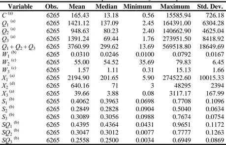
We have also checked for the presence of outliers. Observations for which the factor prices were lower than the 1st centile or larger than the 99th centile have been dropped. Finally, we excluded banks for which less then three observations were available. The final sample consists of 6265 observations on 703 banks. The panel is unbalanced, and includes about 9 observations for each bank. Table 1.1 provides some descriptive statistics of the sample.

15

This approach has also been used by Allen and Liu (2007) and Feng and Serletis (2009).

16

Following an acknowledged approach in the banking literature, we consider physical capital as a variable input. Moreover, Hunter and Timme (1995) found that estimated scale economies are not affected if capital is considered as a quasi-fixed input.

(17)

17

It is worth nothing that Q3 represents, on average, the 26% of total outputs,17

showing the importance of non-traditional activities in the production process of Italian banks. Then, omitting this type of activities could lead to biased results.

TABLE 1.1 – Descriptive statistics of the sample

Variable Obs. Mean Median Minimum Maximum Std. Dev.

C (a) 6265 165.43 13.18 0.56 15585.94 726.18 Q1 (a) 6265 1421.12 137.09 2.45 164391.00 6304.28 Q2(a) 6265 948.63 80.23 2.40 140662.90 4625.04 Q3(a) 6265 1391.24 69.44 1.76 273951.50 8418.92 Q1 + Q2 +Q3 6265 3760.99 299.62 13.69 569518.80 18649.69 W1(b) 6265 0.0310 0.0246 0.0100 0.0792 0.0167 W2 (c) 6265 55.00 54.52 35.69 79.83 6.45 W3 (c) 6265 1.57 1.11 0.31 15.13 1.66 X1(a) 6265 2194.90 201.65 5.90 274522.60 10015.33 X2(d) 6265 640.16 71 3 48295 2394 X3 (a) 6265 39.66 3.88 0.08 3117.17 167.99 S1(b) 6265 0.4062 0.3963 0.0698 0.7708 0.1096 S2(b) 6265 0.2849 0.2828 0.0904 0.5040 0.0634 S3 (b) 6265 0.3089 0.3056 0.0988 0.7674 0.0754 SQ1(b) 6265 0.4395 0.4364 0.0431 0.9651 0.1172 SQ2(b) 6265 0.3047 0.3012 0.0077 0.7777 0.1263 SQ3(b) 6265 0.2558 0.2500 0.0034 0.6949 0.0869 (a)

Millions euro (2000 values) - (b) Ratio - (c) Thousands euro (2000 values) - (d) Units

Si = cost share of input i

SQi = share of output i with respect to total output (Q1 + Q2 + Q3)

1.5 Estimation results

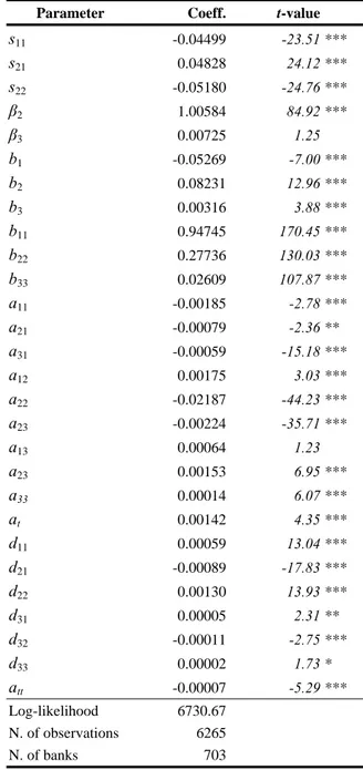
The system (3) has been estimated by maximum likelihood.18 Table 1.2 shows the parameter estimates.19 In a preliminary estimation, the S matrix was found to be not negative semidefinite, then the concavity of the cost function has been imposed by reparametrizing and re-estimating the model, as discussed in Section 1.3. However, the log-likelihoods of the two models are almost the same.20 Most of the 28 parameters are statistically significant at the 1% level.

17

Since all outputs are expressed in (constant) monetary values, we can add them, and compute the share of each output to total output.

18

Note that the cost function does not contain additional parameters with respect to (3); so estimating it along with the input demand system is useless.

19

Estimations have been performed using a program written in GAUSS.

20

(18)

18

Table 1.3 shows the R2 for each estimated equation and for the cost function. The lower value (0.86) is that of the capital equation, probably because of the imperfect measurement of this factor of production by the book value of the fixed assets. Although the cost equation has not been included in the estimated system, its goodness of fit measure reaches a satisfactory value of about 0.92.

TABLE 1.2 – Parameter estimates

Parameter Coeff. t-value

s11 -0.04499 -23.51 *** s21 0.04828 24.12 *** s22 -0.05180 -24.76 *** β2 1.00584 84.92 *** β3 0.00725 1.25 b1 -0.05269 -7.00 *** b2 0.08231 12.96 *** b3 0.00316 3.88 *** b11 0.94745 170.45 *** b22 0.27736 130.03 *** b33 0.02609 107.87 *** a11 -0.00185 -2.78 *** a21 -0.00079 -2.36 ** a31 -0.00059 -15.18 *** a12 0.00175 3.03 *** a22 -0.02187 -44.23 *** a23 -0.00224 -35.71 *** a13 0.00064 1.23 a23 0.00153 6.95 *** a33 0.00014 6.07 *** at 0.00142 4.35 *** d11 0.00059 13.04 *** d21 -0.00089 -17.83 *** d22 0.00130 13.93 *** d31 0.00005 2.31 ** d32 -0.00011 -2.75 *** d33 0.00002 1.73 * att -0.00007 -5.29 *** Log-likelihood 6730.67 N. of observations 6265 N. of banks 703 Dependent variable: C.

*** = significant at the 1% level ; ** = significant at the 5% level; * = significant at the 10% level.

Standard errors computed on the basis of the estimated Hessian of the log-likelihood.

(19)

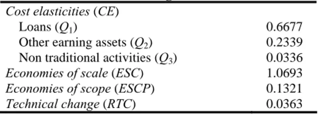
19

Table 1.4 reports the cost elasticities with respect to outputs, scale and scope economies, and the rate of technical change, all computed at the sample means of the variables. Among the three outputs considered, loans show the higher cost elasticity. More precisely, a 1% increase in the production of loans translates into a 0.66% increase in total costs. Conversely, the percentage increase generated by a 1% increase in non-traditional activities is very low (0.03%). The sum of cost elasticities with respect to output equals to 0.94, implying an estimated value of ESC around 1.07, which is very similar to the result (1.09) obtained for Italy by Cavallo and Rossi (2001). This indicates that Italian banks have been characterized by slight economies of scale during the period under study. However, it is interesting to note that at the average total output, which equals to about 3.8 billions euro, economies of scale are not still exhausted.

The value of ESCP is positive (see Table 1.4), implying the presence of economies of scope. Our estimate suggests that producing the three outputs separately translates into an increase in total cost of 13.21% with respect to the cost that would result from the joint production of all outputs. The sign of this finding is consistent with that of Cavallo and Rossi (2001).21 Scope economies, along with a lowering of risk, could explain the trend toward a diversification of activities and income sources followed by many banks in the last years, even through mergers and acquisitions.

Finally, the cost of banks reduced over time at an annul rate of 3.63%. This value is the same as that estimated by Altunbas et al. (1999) when considering the whole European banking system in the period 1989-1996. Then, banks have benefited substantially from technical progress.

Price elasticities of input demands are reported in Table 1.5. Every input demand is inelastic with respect to its own price. Labour seems to be the most sensitive factor of production to changes in price (-0.11). Conversely, deposits show an elasticity that is very close to zero. Regarding cross price elasticities, labour and capital turn out to be substitutes; according to our estimates, if the price of capital increases by 1%, the demand for labour increases by 0.12%. In the opposite case, that is if the price of labour increases by 1%, the demand for capital increases by 0.08%. Also deposits and capital

21

Regarding economies of scope, they report a value of 71.8% (for the whole European banking system), that seems unreasonably high.

(20)

20

are substitutes, but the associated elasticities are much lower. Finally, deposits and labour appear to be complements, although the elasticity is nearly equal to zero.

Overall, we observe that our model generates lower price elasticities (in absolute terms) than those obtained in other studies, such as Hunter and Timme (1995) and Lang and Welzel (1998), both employing a translog specification. However, our price elasticities are comparable to those estimated by Glass and McKillop (1992) and Featherstone and Moss (1994) who used a generalized translog and a normalized quadratic cost function, respectively.

TABLE 1.3 – Goodness of fit

Equation R2

Total Cost (C) 0.9210

Deposits (X1) 0.9995

Labour (X2) 0.9626

Capital (X3) 0.8643

The R2_{values was calculated for each equation as}

1- var(u)/var(Y) where var(u) is the variance of the residuals and var(Y) is the variance of the dependent variable.

TABLE 1.4 – Cost economies and technical

change

Cost elasticities (CE)

Loans (Q1) 0.6677

Other earning assets (Q2) 0.2339 Non traditional activities (Q3) 0.0336

Economies of scale (ESC) 1.0693 Economies of scope (ESCP) 0.1321 Technical change (RTC) 0.0363

TABLE 1.5 – Price elasticities Deposits (X1) Labour (X2) Capital (X3) Deposits (X1) -0.0002 -0.0034 0.0037 Labour (X2) -0.0068 -0.1139 0.1207 Capital (X3) 0.0045 0.0751 -0.0796

(21)

21 1.6 Conclusion

In this paper we have analyzed the production process of the Italian banking industry in the period 1992-2007. Using a large dataset on 703 banks, we have estimated a MSGM system of factor demand equations in order to assess the degree of scale and scope economies and the rate of technical change.

The major findings can be summarized as follows. There is evidence of slight economies of scale. Conversely, cost economies from the joint production of several outputs are quite substantial. Finally, we find a reduction in costs due to technical change of about 3.63% per year.

Based on these findings, we can conclude that Italian banks obtained significant efficiency gains from the consolidation process. Specifically, this process appears to have been driven by cost economies associated to diversification, rather than a reduction in costs due to a larger size. From a policy point of view, this result suggests that the consolidation process should be beneficial to consumers, especially in view of the not remarkable anticompetitive effects of mergers and acquisitions, highlighted by research on market power in the banking industry.

(22)

22

CHAPTER TWO

Testing the “Quiet Life” Hypothesis in the Italian Banking

Industry

2.1 Introduction

During the last two decades the banking sector of many countries has experienced a huge consolidation process. This is due to several reasons, such as technological progress, globalization, and deregulation of banking markets.1 Regarding Europe, crucial factors stimulating the M&A operations have been also the adoption of the Second Banking Directive in 1989 and the implementation of the Economic and Monetary Union.

In Italy the number of banks reduced from 922 in 1998 to 806 in 2007, while in the same period the assets of the whole banking system increased from 1936.71 to 3871.32 billions euro.2 This consolidation trend has raised concerns about its welfare implications, given that the banking market is vital for the whole economic system. Actually, from a theoretical point of view a more concentrated industry could lead to greater market power for banks. Thus, many empirical studies have attempted to estimate the degree of competition of the banking sector, often using the methodologies proposed by the so-called New Empirical Industrial Organization (NEIO).3

However, there is a related potential problem stemming from the exploitation of market power. It is the possibility, first stressed by Hicks (1935) and known in the literature as the “quiet life” hypothesis (QLH), that firms with higher market power put less effort in pursuing cost efficiency: instead of taking advantage of their favourable position by also cutting costs, in order to gain higher profits, they prefer to enjoy a “quite life”. However, as pointed out by Berger and Hannan (1998), there are several

1

See Berger et al. (1999) for a review on causes and implications of consolidation in the financial services industry.

2

Bank of Italy data (current values).

3

With reference to the European countries see, among others, Molyneux et al. (1994), De Bandt and Davis (2000), Shaffer (2001), Bikker and Haaf (2002), and, for Italy, Coccorese (2005, 2008b).

(23)

23

other reasons for which firms with more market power would be less efficient. For example, their managers could overexpand some expenses, especially in order to preserve market power.

Surprisingly, this issue has received relatively little attention in the empirical literature, and only some recent studies have tried to test the QLH in banking. The aim of this paper is to contribute to this stream of literature focusing on the Italian banking industry for the period 1992-2007.

Using a two-step procedure, we first estimate bank-level cost efficiency scores and Lerner indices by means of a stochastic frontier model. Then we use the estimated market power measures, as well as a vector of control variables, to explain cost efficiency, also dealing with the potential endogeneity of the Lerner index. Our results support the prediction of the QLH, as banks’ market power appears to negatively affect their cost efficiency, even if the overall impact is not particularly remarkable in magnitude. This means that the “quiet life” behaviour of Italian banks, although existing, does not lead to a noteworthy loss of efficiency.

Our analysis is characterized by a number of worthy features. First, it considers a single country, so that the results of the empirical analysis are more reliable because of the homogeneity of various factors (legal, historical, cultural, social) that usually play a crucial role in influencing firms’ behaviour but are more difficult to be caught in a cross-country framework. Second, we estimate efficiency scores making use of two different stochastic frontier models, namely the standard Battese and Coelli (1992) methodology and the Aigner et al. (1977) approach, and perform the second step estimation by means of both a tobit model (the most widely adopted approach) and a logistic model (which, in our view, is more appropriate in this framework). The use of various techniques allows to check the robustness of our empirical evidence. Finally, we carry out some estimations also for sub-samples of banks, in order to assess possible different behaviours according to their type, location and size.

The paper is organized as follows. Section 2.2 offers a review of the literature on the estimation of market power in banking and the relationship between market power and efficiency. The methodologies used to estimate both banks’ market power and cost efficiency, and to test the QLH, are described in Sections 2.3 and 2.4, respectively.

(24)

24

Section 2.5 illustrates data and variables, while the results are presented and discussed in Section 2.6. Finally, Section 2.7 draws some conclusions.

2.2 Market power, efficiency, and their relationship: a review of the banking literature

At the start, the assessment of competition in banking has been essentially based on the “structure-conduct-performance” (SCP) paradigm, first proposed by Mason (1939) and Bain (1951), according to which the performance of an industry depends on the behaviour of incumbent firms, which in turn is determined by the market structure, usually proxied by the level of concentration.

For the empirical implementation, this paradigm has taken a “structure-performance” (SP) form, since the standard practice has been to estimate a relationship between a measure of performance (in terms of profits or prices) and a concentration index.4 In this framework, a statistically significant and positive coefficient of the concentration variable is interpreted as evidence of a cooperative behaviour among firms that allows them to exploit their market power at expense of customers.

While such a simplified version of the model can be theoretically justified (e.g. Cowling and Waterson, 1976), it has led to undervalue the role of firms’ conduct in determining the equilibrium of the industry. The most important challenge to the SP hypothesis is the contestability theory of Baumol et al. (1982). According to these authors, an industry can reach competitive outcomes, whatever the level of concentration, if potential entrants are able to exert an adequate competitive pressure on incumbent firms.

Another criticism to the SP paradigm comes from the “efficient structure” (ES) hypothesis, suggested by authors like Demsetz (1973) and Peltzman (1977). They remark that a higher level of market concentration could be the result of differences in efficiency among firms or across markets. Firms that are more efficient get both higher market shares and profits, so that we observe a spurious positive relationship between profits and concentration. In other words, the SP and ES hypotheses take different

4

(25)

25

variables as exogenous: concentration and efficiency, respectively (Berger and Hannan, 1989).

Based on the shortcomings of the SCP approach, the New Empirical Industrial Organization (NEIO) has developed several methodologies to derive a conduct parameter as a measure of the market power exerted by firms. One possibility is to estimate a simultaneous model of demand and supply equations, where the conduct parameter is represented by a conjectural variation coefficient that can assume different values depending on the degree of market power prevailing in the industry. Pioneered by Iwata (1974), this approach has been developed by Bresnahan (1982) and Lau (1982),5 and applied to the banking sector by many authors.

Along the line of NEIO, Panzar and Rosse (1987) propose a methodology based on the estimation of a reduced form revenue equation, which includes the prices of the inputs among the regressors. The sum of the estimated elasticities of revenues to factor prices provides the so-called H-statistic, representing a conduct parameter that can range from negative values (monopoly or collusion) to one (perfect competition). The

H-statistic only allows to discriminate among different market hypotheses, but it has

been shown that, under specified assumptions, this index can be interpreted as a continuous measure of competition (Vesala, 1995, p. 56; Bikker and Haaf, 2002, p. 2203).

Another NEIO approach for assessing the degree of market power in banking is based on the calculation of the Lerner index, where the marginal cost (needed for its assessment) is obtained by means of the estimation of a cost function.6 One advantage of this methodology is to provide a bank-level measure of market power, whose evolution over time can also be easily traced.

While several empirical studies have focused on the estimation of market power of banks, the attention towards its influence on efficiency is much more recent and leads to assorted results.

In general terms, the link between market structure and efficiency was first postulated by Hicks (1935), who argued that monopoly power allows managers to enjoy

5

∑

+

(

)

2 3 3

(

)

2 1 1 1 ln ln ln ln 2 QQ it h k hk hit kit TT Q W W TREND α α α = = ⎧ ⎫ + _⎨ + + _⎬ ⎩

∑∑

⎭ 3 1 ln ln ln ln Qh it hit TQ it h Q W TREND Q α α = +

∑

+ 3 1 ln ln Th hit it h TREND W α ε = +

∑

+ (1)

where i = 1,...,N and t = 1,...,T index banks and time, respectively, C is the total cost, Q is the output, Wh are the factor prices, and TREND is a time trend included to take into

account technical change. Finally, εit = vit + uit is a two-components error term, where vit

(30)

30

modelled as a function of time, i.e. uit = ui exp[–γ (t–Ti)], where ui is a truncated normal

distribution with mean μ and variance σu2.

One shortcoming of the above specification is that it imposes an a priori time path to the efficiency scores, which depends on the estimation of the γ parameter. Therefore, as robustness check, for the pooled sample we also estimate the stochastic frontier model as suggested by Aigner et al. (1977) and Meeusen and van Der Broeck (1977), where the uit term – assumed to be distributed as a half-normal random variable – is free to

vary over time without any a priori assumption.

Regarding the cost function, by symmetry of the Hessian we have αhk = αkh. In order

to correspond to a well-behaved production technology, the cost function needs to be linearly homogeneous, non-decreasing and concave in factor prices, and non-decreasing in output. With the symmetry restrictions imposed, necessary and sufficient conditions for our translog cost specification to be linearly homogeneous in input prices are:7

∑

= = 3 1 1 h h α ,

∑

= = 3 1 0 k hk α (h = 1,2,3),

∑

= = 3 1 0 h Qh α ,

∑

= = 3 1 0 h Th α .

The cost efficiency scores have been estimated as CE_it =E

[

exp

(

−u_it

)

|ε_it

]

.8 Since

uit ≥ 0, CEit ranges between 0 and 1, with CEit = 1 characterizing the fully efficient firm.

Employing the parameters resulting from the estimation of the cost function, we can compute the marginal cost for each bank and time period as

3 1 ln ln ln ln ln it it it it it it it it Q QQ it Qh hit TQ h it C C C MC Q Q Q C Q W TREND Q α α α α = ∂ ∂ = = ∂ ∂ ⎛ ⎞ =_⎜ + + + _⎟ ⎝

∑

⎠ (2)

and the Lerner index as

7

We imposed symmetry and homogeneity restrictions during the estimation process, and checked the other properties after estimation.

8

(31)

31 it it it it P MC P LERNER = − ₍₃₎

where Pit is the price charged on the output. Theoretically, the Lerner index can vary

between 0 (in case of perfect competition) and 1.

2.4 Testing the “quiet life” hypothesis

We implement the test of the QLH for Italian banks by regressing the cost efficiency scores (CE) on the estimated Lerner index (LERNER) as well as a set of market-level and bank-level control variables. A negative and statistically significant coefficient of the variable LERNER can be interpreted as evidence of the validity of the QLH.

As market-level variables we consider:

• the growth rate of GDP (GDPGROWTH). It is included to take into account the influence of the business cycle on efficiency. In expanding and dynamic markets, banks can count on an increasing flow of demand that, if captured, could help to better exploit their (branch and/or network) size and hence improve efficiency. At the same time, competition among banks is expected to be stronger, so banks need to be prepared to take every opportunity that allows to enlarge the clientele, and could be forced to forgo efficiency on the grounds of short-run profitability. As a result, we can not anticipate the sign of this variable;

• the population density (POPDENS), given by the number of inhabitants per square kilometre. On one hand, in markets with high density of people it should be less costly to offer banking services; on the other hand, dealing with more customers could generate inefficiencies because of the difficulty of meeting all customers’ requirements with good standards. Hence, the sign of this variable is not a priori determinable.

In order to have one value for each of the previous regressors, for all banks that operate in more than one geographical market the corresponding data have been

(32)

32

weighted according to the distribution of branches.9 As relevant markets, we consider the 20 Italian regions.

The bank-level variables are:

• the ratio between loans and total assets (LOANASS). Contrary to other bank assets (e.g. securities), lending requires more effort and organizational capabilities by the staff. If not properly performed, it could therefore generate inefficiencies;

• the deposits to assets ratio (DEPASS). Deposits are the main source of financing for banks, but they also ask for a good organization in order to be gathered and well managed. For the same reasoning as above, a higher fraction of deposits among liabilities could then produce inefficiencies on the cost side. As a result, we expect a negative coefficient for this variable too;

• the natural logarithm of the number of branches (lnBRANCHES). A widespread branch network involves the creation and management of a retail organization and the work of a possible large number of people. This could have a negative (or positive) impact on cost efficiency, depending on the coordination and organizational problems (or opportunities) linked to a bigger dimension. Under this point of view, branches can be also regarded as a good proxy for banks’ size;10

• the natural logarithm of total assets per branches (lnASSBR). This variable measures the average degree of capacity utilization of banks’ branches. If economies of scale at the branch level exist, banks that are able to manage more assets per office should be more efficient, and this would involve a positive sign for the estimated coefficient.

In addition to these bank-level variables, we also control for the influence of bank type and bank location on efficiency. To this purpose, we introduce two groups of zero-one dummy variables: the first considers whether a given credit institution is a commercial, popular or cooperative bank (the latter representing our reference group);

9

For an analogous choice, see Maudos (1998) and Coccorese and Pellecchia (2009).

10

We prefer to proxy size with branches rather than total assets also because the latters are employed as a measure of the output Q in the cost function (see below).

(33)

33

the second records its location (North-West, North-East, Centre, South; here the first variable is assumed as reference).11

Given that CEit lies between 0 and 1, an estimation using OLS would not be

appropriate. Hence, some authors12 employ a double-censored tobit specification, in accordance with what is suggested by Kumbhakar and Lovell (2000).13

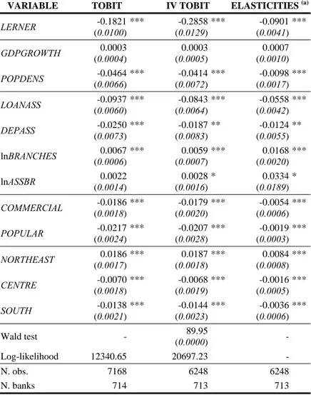
As discussed in Section 2.2, the ES hypothesis postulates a causal relationship going from efficiency to market power. Thus, in our econometric model the variable LERNER could be endogenous. To deal with this possibility, besides a standard tobit specification, we also estimate an instrumental variables (IV) tobit model, where the Lerner index is instrumented using its first lag. Possible endogeneity can be tested by means of a Wald test (Wooldridge, 2002, pp. 472 ss.).

However, the tobit model is appropriate only when bounds on the dependent variable stem from non-observability. The fact that the dependent variable can take values in a given range is not per se a good motivation to use this type of model (Maddala, 1991). This is also the view of McDonald (2009), who shows that, if there are no observations for which CEit = 0 or CEit = 1 (as very often happens in empirical

applications), estimating a double-censored tobit model is the same as estimating a linear regression model, since the two likelihood functions coincide.

Therefore, as an alternative specification, we also estimate the following logistic regression:

( )

it it it it _x x CE φ β β + + = ' _' exp 1 exp , (4)

where xit is the same vector of regressors used for the tobit model, β is the vector of

parameters, and φit is an i.i.d. error term with mean zero and variance σφ2.14 Again, to

11

Banks operating in more than one macro-region have been assigned to the area where they manage the higher fraction of branches.

12

For example, see Koetter et al. (2008) and Turk Ariss (2010).

13

«Since the dependent variable ... is bounded by zero and one, ... either the dependent variable must be transformed prior to estimation or a limited dependent variable estimation technique such as tobit must be employed». See Kumbhakar and Lovell (2000), p. 264.

14

(34)

34

cope with possible endogeneity problems, we estimate this model also instrumenting the Lerner index by its first lag.

2.5 Data and variables

Our sample of Italian banks is drawn from the database Bankscope,15 and covers the period 1992-2007. In this database, balance sheet and profit and loss account figures are reported for each bank both in consolidated and unconsolidated form.16 We have made use only of unconsolidated data, treating holding banks and their affiliates as separate decisional units. Since the organizational type was also available, we have selected only commercial, cooperative and popular banks, and dropped those observations for which relevant variables were not available.

As consistency check, and in order to include in the sample the number of branches of each bank (which is seldom reported in Bankscope), the data have been matched with those included in the yearly official lists of operating banks, available from the Bank of Italy. We dropped the observations that did not pass this test.

Following the intermediation approach to banking costs (Sealey and Lindley, 1977), the three inputs we consider in the cost function are: deposits, labour, and capital. Cost figures corresponding to these inputs are interest expenses, personnel expenses, and other operating costs, respectively. The last variable has been computed subtracting labour costs from all operating costs (which are net of financial expenses).

The price of deposits (W1) has been computed dividing interest expenses by the sum

of deposits, money market funding and other funding. The price of labour (W2) is

defined as the ratio between personnel expenses and total assets.17 Finally, the price of capital (W3) has been set equal to the ratio between the other operating costs and the

value of the fixed assets.

15

This database is distributed by Bureau van Dijk Electronic Publishing (BvDEP) and is a widely used data source in empirical studies on banking.

16

The consolidated data refer to holding banks and their affiliates.

17

(35)

35

As in Shaffer (1993) and Angelini and Cetorelli (2003), the output (Q) is proxied by the value of the total assets. The (single) output price (P) is computed as the ratio between total revenues (interest income plus net non-interest income) and total assets.

In order to correct for outliers, the observations for which the output and/or factor prices were lower than the 1st centile or larger than the 99th centile have been dropped. We have also discarded those banks for which less then three observations were available. After the data selection process, we have been left with 7168 observations on 714 banks. The panel is unbalanced, due to sample selection, consolidation, new entries and bankruptcies. On average, it includes 10 observations for each bank (see Table 2.1).

Some descriptive statistics regarding the variables used in the two estimation steps are provided in Table 2.2.

2.6 Estimation results

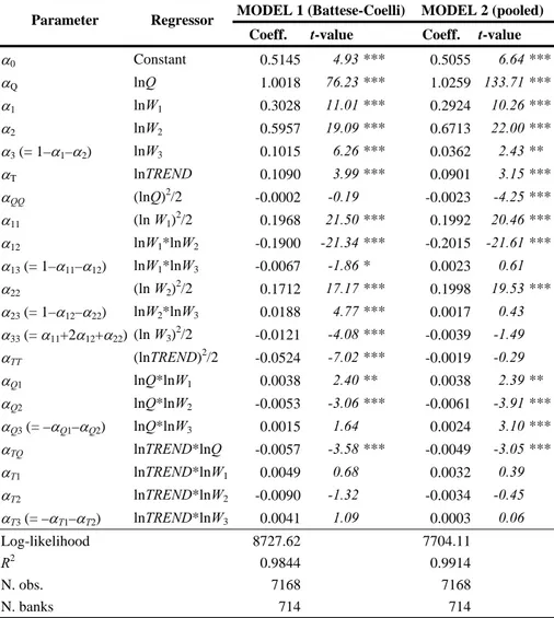
Consistent with the standard procedure characterizing the stochastic frontier analysis, Equation (1) has been estimated by maximum likelihood. Results for both the Battese-Coelli and the pooled stochastic frontier models (Model 1 and 2, respectively) are reported in Table 2.3. Almost all the estimated parameters are statistically significant at the 1% level.

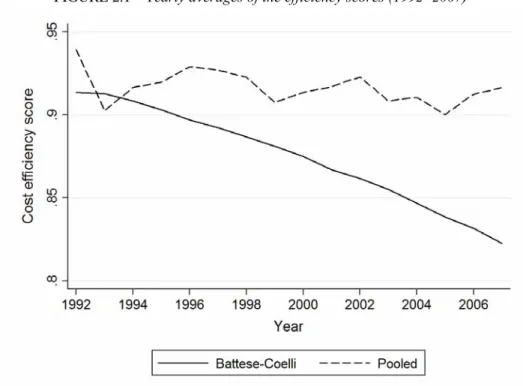
Yearly averages of the efficiency scores and the Lerner indices for both models are presented in Table 2.4. As expected, cost efficiency scores derived from the Battese-Coelli model exhibit a clear (decreasing) trend, while those coming from the pooled estimation show an irregular pattern over time (see Figure 2.1).

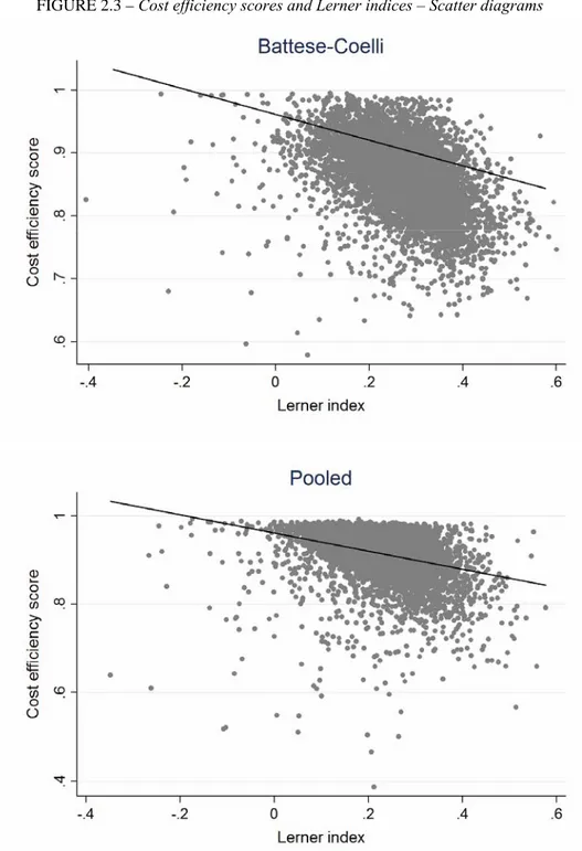
In contrast, the trend of the Lerner index is clearly upward, indicating that the market power of the Italian banks has increased during the time interval under study (see Figure 2.2).18 More precisely, the yearly average of the Lerner index ranges between 0.16 (in 1992) and 0.34 (in 2007) when considering Model 1, and between 0.15 and 0.27 for Model 2.

18

This finding is consistent with the results (for Italy) of Maudos and Fernández de Guevara (2007), who employ the Lerner index as a measure of market power, and of Van Leuvensteijn et al. (2007), who use the Boone indicator.