Studies of CMS data access patterns with machine learning techniques

(1)

Alma Mater Studiorum · Universit`

a di Bologna

Scuola di Scienze

Dipartimento di Fisica e Astronomia Corso di Laurea in Fisica

Studies of CMS data access patterns with

Machine Learning techniques

Relatore:

Prof. Daniele Bonacorsi

Presentata da:

Silvia De Luca

Sessione II

(2)

Sommario

Questa tesi presenta uno studio dei patterns di accesso allo storage su Grid in analisi distribuita da parte dell’esperimento CMS all’acceleratore LHC.

Questo studio spazia dall’analisi approfondita dei patterns di accesso ai file di CMS in passato (la cosiddetta “popularity”), fino all’utilizzo di un sistema di Supervised Machine Learning di tipo classificazione per prevedere i patterns di accesso ai dati dell’esperimento in futuro - con attenzione a particolari tipi di dati. L’esperimento CMS ha completato la sua prima fase di presa dati a LHC (Run-1) e, dopo un lungo periodo di shutdown (Long Shutdown 1) è iniziata nel 2015 la raccolta dei dati prodotti da collisioni protone-protone a 13 TeV del centro di massa nel periodo detto Run-2. I workflow di CMS vengono es-eguiti su centri di calcolo (Tiers) di Worldwide LHC Computing Grid (WLCG), e in particolare l’analisi distribuita supporta le attività di centinaia di utenti al giorno. Le applicazioni CMS accedono a diversi tipi di dati ospitati sui sistemi di storage (disco) ai Tiers. Lo studio dettagliato di come questi dati vengono acceduti, in termini di tipolo-gia, livello di Tier che li ospita e periodi di tempo in cui vengono acceduti permette di ottenere informazioni preziose sull’efficienza di utilizzo dello storage Grid di CMS, e in ultima analisi estrarre da esse suggerimenti per azioni concrete (ad esempio, pulizia delle cache disco e/o ulteriori repliche dei dati). In tal senso, l’applicazione di tecniche di Ma-chine Learning permette di complementare quest’attività: l’apprendimento dei patterns di accesso a dati passati consente di costruire modelli con potenzialità predittive sugli accessi futuri.

Il Capitolo 1 fornisce un’introduzione sulla Fisica delle Alte Energie e su LHC.

Il Capitolo 2 descrive il modello di calcolo di CMS, con attenzione particolare al data management, introducendo anche il concetto di popolarit`a.

Il Capitolo 3 descrive lo studio dei patterns di accesso ai dati di CMS con diverse “view” e livelli di approfondimento.

Il Capitolo 4 offre un’introduzione a concetti di Machine Learning e spiega come ven-gono applicati in questo studio, descrivendo approcci seguiti e risultati ottenuti.

(4)

Abstract

This thesis presents a study of the Grid data access patterns in distributed analysis in the CMS experiment at the LHC accelerator.

This study ranges from the deep analysis of the historical patterns of access to the most relevant data types in CMS, to the exploitation of a supervised Machine Learning classification system to set-up a machinery able to eventually predict future data access patterns - i.e. the so-called dataset “popularity” of the CMS datasets on the Grid - with focus on specific data types.

The CMS experiment has completed its first data taking period at the LHC (Run-1) and, after a long shutdown (LS(Run-1), is now collecting proton-proton collisions data at 13 TeV of centre-of-mass energy in Run-2. All the CMS workflows run on the World-wide LHC Computing Grid (WCG) computing centers (Tiers), and in particular the distributed analysis systems sustains hundreds of users and applications submitted ev-ery day. These applications (or “jobs”) access different data types hosted on disk storage systems at a large set of WLCG Tiers. The detailed study of how this data is accessed, in terms of data types, hosting Tiers, and different time periods, allows to gain precious insight on storage occupancy over time and different access patterns, and ultimately to extract suggested actions based on this information (e.g. targetted disk clean-up and/or data replication). In this sense, the application of Machine Learning techniques allows to learn from past data and to gain predictability potential for the future CMS data access patterns.

Chapter 1 provides an introduction to High Energy Physics at the LHC.

Chapter 2 describes the CMS Computing Model, with special focus on the data man-agement sector, also discussing the concept of dataset popularity.

Chapter 3 describes the study of CMS data access patterns with different depth levels. Chapter 4 offers a brief introduction to basic machine learning concepts and gives an introduction to its application in CMS and discuss the results obtained by using this approach in the context of this thesis.

(5)

Chapter 1 High Energy Physics at the LHC

1.1 The Standard Model

The Standard Model [3][4], developed in 1970, incapsulates the remarkable theories and discoveries of particles physics since 1930, it has an important feature: it is verified by all available data, secondly it gives a unified description in terms of quantum field of all the interaction of known particles (except gravity): Electroweak and Quantum Chro-modynamic; Gravitation si excluded because SM hardly faces phenomena at Planck’s scale of energy 10−19GeV (of interest in cosmology). The SM also describes all particles and splits them into two main classes according to their intrinsic angular momentum: fermions, that have half-integer spin, and bosons which have integer spin. There are twelve fermions respectively six leptons and six quarks, the building blocks of matter. Moreover, for every particle there is its own antiparticle: a particle that differs only for opposite internal quantum numbers. Quarks can have three different colors (red, blue, green)and only mix in such ways as to form colourness objects, while lepton have ei-ther unitary or null electric charge and they can be organized in three generations (with associated neutrino):

νe νµ ντ

e µ τ

!

Electron, muon, tau (second row) and their associated neutrino (first row) but there is a phenomena by which neutrinos can evolve into a different kind i.e. νe becomes νµ and

so on. Electron, muon and tau interact by both electromagnetic and weak force whereas neutrinos only by weak force. Quarks interact by strong force that is regulated by colour charge. We have in this model a very detailed description of fundamental interaction: the strong force, the weak force, the elctromagnetic force and the gravitational force. They work over different ranges and have different strenghts: gravity is the weakest but it has and infinite range; the electromagnetic force also has infinite range but is many time

(6)

stronger than gravity. The weak and strong forces are effective only over a very short range and dominate only at the level of subatomic particles. Three of the fundamental forces result from the exchange of force-carrier particles, called bosons. Each fundamenta force has its own boson: the strong force is carried by the gluon; the electromagnetic force is carried by the photon; the interaction of weak force is due to the W and Z bosons; the corrisponding force-carrying particle of gravity should be the graviton but not yet found.

There are also questions that it does not answer regarding to: what is dark matter, what happened to the antimatter after big bang, how it is possible that there are three generations of quarks and leptons with such differen masses, etc. A great goal achived was the confirmation of Higgs boson existence, an essential component of the Standard Model.

(7)

1.2 CERN and the LHC

The European Organization for Nuclear Research, known as CERN [1][2] is a research organization that operates the largest particle physics laboratory in the world; the term CERN is also used to refer to the laboratory. In 1954, 12 European nations came together to sign the convention officially forming CERN and nowadays has 22 member states. It is concived to study the basic costituents of matter - the fundamental particles; a num-ber of clues about how the particles interact and insights into the fundamental laws of nature came from collisions between particles (close to the speed of light). At CERN purpose-built particle accelerators and detectors are used to investigate. Accelerators boost beams of particles to high energies before the beams are made to collide with each other or with stationary targets. Detectors observe and record the results of these collisions. Initially CERN was focussed of pure physics research ad understanding the inside of the atom. Today we go beyond “nuclear” world and aim to explore the particle physics (the fundamental costiuents of matter and the forces between them) and much more ranging from high-energy phisics, from studies of antimatter to the possible effects of cosmic rays on clouds. The particle physics have described the fundamental structure of matter using the Standard Model: describes how everything that we observe in the universe is made from a few basic blocks called fundamental particles, governed by four forces. Then, at CERN accelerators are used also to test the predictions of standard model. One takes account that the model only describes the 4% of the known universe. CERN is not only particle physics, one remarcable thing happened in 1989 when Tim Berners-Lee, a British scientist, invented the World Wide Web (WWW); its initial pur-pose was to meet the demand for automatic information-sharing between scientists in universitied and institutes around the world. The first web site described the basic fea-tures of the web; the software of World Wide Web was put in the public domain in 1993. Other physics topics are for example: compositeness, the high energy collisions at LHC could be the key to find a possible substructure for subatomic particles; cosmic rays that are rays of charged particles which energy is far higher than LHC’s; dark matter, a miste-rious matter that makes up most of the universe; extra dimensions, gravitons; heavy ions and quark-gluon plasma to recreate similiar condition of universe just after the Big Bang. The Large Hadron Collider [5][6] is the world’s largest and most powerful particle accel-erator. It first started up on September 2008, and stands as the main component of the accelerator complex. The LHC, built in a tunnel buried 175m unerground, consists of a 27 kilometer ring of superconducting magnets with a number of accellerating structure to boost the energy of the particles along the way. Inside the accelerator, two high-energy particle beams travel at close to the speed of light before they collide. The beams are stored for hours; during this time collisions take place inside the four main LHC experi-ments. The beams travel in opposite directions in separate beam pipes - two tubes kept at ultrahigh vacuum. They are guided around the accelerator ring by a strong magnetic

(8)

field maintained by superconducting electromagnets. The electromagnets are built of coils that operate in a superconducting state, efficiently conducting electricity without resistance or loss of energy. This requires a connection to huge cryogenic stystems which cool the magnets at −271.3C.

Figure 1.2: Graphic representation of LHC tunnel.

The LHC is a proton-proton and heavy ion collider. At the start of the accelerator’s complex there is a bottle full of gaseous hydrogen from which the ionization process starts using a duoplasmatron to generate protons. The idea of a circular accelerator arises from the need to work at high energy level. Particle acceleration process is made possible by and electric field generated by a system of electrods alternating poles. At each step, the proton increases its velocity therefore the time interval from previous step to the next is each time shorter. A solution is the linear accelerator model LINAC [7]. In real application, the acceleration process is performed by using resonant cavities and radio-frequency generators. Thus with a LINAC could be hard reaching energies about TeV, because it entails a longer accelerator. To avoid this incovenient, scientists thought about a “ring” structure composed by linear accelerator steps (LINAC) connected to each other by magnetic dipole to bend proton’s trajectory and to keep them in line. The LHC dimensions are aimed at minimizin the loose of energy under synchrotron radiation which depends on the bending ray.

Protons are allowed to enter the LHC accelerator [6] when they reach a 450 GeV energy. To reach this target there are four pre-accelerating steps represented in Fig.1.3:

• LINAC2 (1978,36m in circumference): from the bottles with gasseous hydrogen to 50MeV energy;

(9)

Figure 1.3: Schematic representation of accelerators complex

• PSB (Proton Synchrotron Booster,1972,157m in circumference): from LINAC2 to 1,4GeV energy;

• PS (Proton Synchrotron): from 1,4GeV to 25GeV;

• SPS (Super Proton Synchrotron,1978,36m in circumference): from 25GeV to 45GeV; • LHC (Large Hadron Collider): to theoretical 14TeV ;

Protons quit SPS from two different injection points. Most of LHC ring is composed by magnets, there are text two different circles (with distinct magnetic fields) with the purpose to keep protons running in clockwise and counterclockwise. Those two parallel rings cross into only four points namely where the main experiments are located. In more detail, as already mentioned, the layout of straight sections depends on the specific use of the insertion, for example:

- physics events such as beam collision; - injection;

- beam dumping etc.

One of LHC characteristic machinery is its Vacuum System [8], as collisions against gas molecules must be avoided. LHC gets three of those: insulation vacuum for cryomag-nets, insulation vacuum for helium distribution line (QRL), beam vacuum. At cryogenic

(10)

temperatures, in the absence of any significan leak, the pressure will be stabilised aroud 10−4P a. The requirements for the beam vacuum are much more stringent, driven by the requested beam lifetime and background to the experiments. The requirements at cryogenic temperature are expressed as gas densities and normalised to hydrogen, should remain below 1015_H

2m−3 to ensure the required 100 hours beam lifetime. All three

vac-uum system are subdivided into sectors by vacvac-uum barriers for the insulation vacvac-uum and sector valves for the beam vacuum. The beam vacuum is divided in sectors of var-ious lengths. A number of dynamic phenomena have to be taken into account for the design of the vacuum system for example synchrotron radiation and electron clouds. A crucial task of experiments in LHC is to make collisions detections. The beams are made up of proton bunches and each one can circulate for many times during the same run; the experiments’ detectors are synchronized along the collisions through a clock whose fundamental frequency coincides with bunches’ position within their trajectory. The protons distribution is choosen to make collision exactly in the middle of detector, how-ever not all protons collide at once so to optimize significant events, one can do basically three things: squeezing bunches is needed to make bunches more compact and aligne the beams; encrease the number of protons in a bunch; raise the number of bunches per run. Each proton beam at full intensity will consist of 2808 bunches; each bunch will contain

Figure 1.4: Main parameters of the LHC.

1.15 ∗ 1011 _{protons at the start of nominal fill. Total beam energy at the maximum is}

352MJ. The bunches are generally far about 25ns from each other; however there are some holes in the bunch structure, the biggest is the beam abort gap of 3µs. This is there to give to the beam bump kickers time to get up to full voltage. There are also other smaller gaps in the beam which arise from similiar needs from the SPS and LHC injection kickers.

(11)

1.3 Experiments at the LHC

Four major experiments at the LHC use detectors to analyse a multitude of particle producted during collisions. The largest particle detectors are those used by the ATLAS and CMS collaborations, to explore a large variety of phenomena at the highest LHC energy scales. ATLAS and CMS, along with other experiments operating at the LHC, are briefly presented in the following.

ALICE (A Large Ion Collider Experiment) [9][10] is a detector designed for heavy-ion collisheavy-ion. It is built to study the physics of strongly interacting matter at extreme energy densities, where a phase of matter called quark-gluon plasma is formed. The quarks, as well as the gluons, seem to be bounded permanently together and confined inside composite particles, such as protons and neutrons. Collisions in the LHC are such hot that recreate in laboratory condition similiar to those just after the big bang. Under these conditions, protons and neutrons melt, freeing the quarks from their bonds with the gluons, thus creating the quark-gluon plasma. The existence and properties of that phase are key issues in the theory of quantum chromodynamics (QCD), understanding the phenomenon of confinement, etc. ALICE studies such state of matter as it expands and cools, and how it ultimately gives rise to the particles we actually observe. The ALICE detector is 26m long, 16m high and 16m wide.

ATLAS [11][12] is the other LHC general-purpose detector; beams of particles from the LHC collide at its detector centre producing debris as new particles, which flow out of the collision point in all directions. Six different detecting subsystems arranged in layers around the collision point record the trajectory, momentum, and energy of the particles. A huge magnet system bends the tracks of charged particles so their momenta can be measured. ATLAS uses a trigger system to tell the detector which events to record and which to reject. Data-acquisition and computing systems are used to collect, handle and analyse the collision events recorded. The ATLAS detector is 46m long, 25m high and 25m wide.

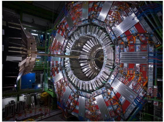
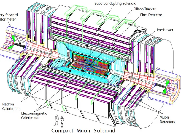
CMS (Compact Muon Solenoid) [13] has a broad physics scope ranging from in-depth studies of the Standard Model to searching for new physics. ATLAS and CMS share the same physics goals, but attack them with detector of quite differ-ent conception. The CMS detector layout is designed around a huge solenoid, a cylindrical coil of superconducting cable that generates a field of 4 tesla and this is confined by a steel yoke. The CMS detector is 21m long, 15m wide and 15m high. LHCb (Large Hadron Collider Beauty) [14][15] is specialised in investigating the slight differences between matter and antimatter by studying the quark b (beauty). LHCb uses a series of subdetectors to mainly detect forward particles. LHCb is

(12)

composed by a sophisticated spectrometer and planar detectors; it is 21m long, 10m high and 13m wide.

LHCf (Large Hadron Collider Forward) [16] uses forwards particles thrown by collisions in the LHC as a source to simulate cosmic rays in laboratory conditions. Cosmic rays are a natural source of charged particles: while colliding with high atmosphere, a cascade of particle is produced and reaches on Earth’s surface. LHCf consists of two detectors which sit along the LHC beamline, at either side of the ATLAS collision point: this location allows the observation of particles at nearly zero degrees to proton beam direction. Each detector is 30cm long 80cm high and 10cm wide.

TOTEM (Total elastic and diffractive cross-section measurement) [18][19] is about taking measurements of protons as they emerge from collisions at small angles, a region known as forward direction, and is inaccessable by other LHC experiments. It is equiped of four particle telescopes and 26 Roman pot detectors, spread around the CMS interaction point. The telescopes use cathode-strip chambers and Gas Electron Multipliers to track the particles emerging from CMS collisions. Roman Pots with silicon sensors perform measurements of scattered protons.

MOEDAL (Monopole and Exotics Detector at the LHC) [20] searches magnetic monopole, a hypothetical particles with a magnetic charge. This monopole detector is an array of 400 modules, each consisting of a stack of 10 sheets of plastic nuclear-track detectors. This detector is deployed around the same intersection regions as the LHCb detector. The magnetic monopoles, if they exist, would rip through the detector, breaking long-chain molecules in the plastic nuclear-track and creating a minute trail of damage through all 10 sheets. Another research is for highly ionizing stable massive particles, predicted by the Standard Model.

(13)

Chapter 2 The CMS Experiment

2.1 The CMS detector

Figure 2.1: Picture of the CMS detector while open.

The Compact Muon Solenoid detector [21] works at the LHC at CERN. It is a multi-purpose detector designed to proton-proton (and lead-lead) collisions. Main CMS work-parameters are: centre of mass energy (14Tev) and luminosity 1034_cm−2_s−1_{. The}

(14)

CMS detector is a stratified fashioned structure consists of five layers: the tracker, the electromagnetic calorimeter, the magnet, the hadronic calorimeter, and the muon system. This is planned to stop, track or measure a different kind of particle derived from early collision. The detector uses a powerful solenoid that bends the trajectory of charged particles. Data given by the detector are stored and then used to recreate what happens at the core of the collision; to do so a Trigger and a Data Acquisition System are needed. When collisions at maximum designed energy occur, 109 events per second will result. So, a significant number of events take place but the on-line selection process has to trigger only 100/s will be saved. This makes and outstanding necessity for a custom electronics capable both to manage high data flux and being able to make extremely careful selections.

The detector design addresses to those general requirements: - A high performance system to identify and track muons;

- A high resolution electromagnetic calorimeter to detect and measure elctrons, positrons and photons;

- A high quality tracking system for momenta measurements;

- A hermetic hadron calorimeter, designed to entirely surround the collision and prevent particles escaping;

Among the stored data there are the momentum and energy of particles; then, by their combination one know what type of particle is and, by tracing back patterns, at least its mass.

It follows a brief description of each system. Tracker

The Tracker [22] is the innermost element of the detector and its task is to detect muons, electrons, hadrons and particles coming from decay. This is made entirely of silicon-based technologies. Particles leave traces of energy that allow to chart their flight paths (position) which are spiral shaped and their curvature reveals their momenta. During momentum measurement, the interaction between the tracker and the particles must be least as possible. The tracker is endowed with two types of technologies for particle detection: pixels and miscro-strips. Outside the detector the signals are transferred through optic fibres cables. Moreover, a second measurement of momentum is performed by an outer muon chamber system, it allows to have a reconstruction mean efficiency about 92%.

Electromagnetic Calorimeter: ECAL

The CMS electromagnetic calorimeter [23] plays a leading role studying the elec-troweak symmetry breaking and detection of two-proton decay and of electrons

(15)

(16)

and positrons coming from Ws and Zs decay. It is main based on scintillating tungstate P bW O4 crystals structure that covers the entire solid angle, and offers

advantageous features:

– It is a fast scintillator (fast light emission); – High performance energy resolution;

– Short radiation leght;

– Easy production process from raw materials;

The light produced by particles hitting the tungstate crystals must be recorded. This operation is performed by Avalanche Photo Diodes (APDs) places around the calorimeter (barrel region) and by Vacuum Photo Triodes (VPTs) at the endcaps. In front of the endcaps there is a preshower detector made of two lead silicon detector layers to distinguish single high-energy photons from pairs of low-energy photons. The photons are detected by a sensor and it is possible to estimate their initial energy.

Hadron Calorimeter: HCAL

The combined CMS calorimeter system examines the direction and energy of stan-dard model particles. The Hadron Calorimeter [24] measures mainly hadron jets, neutrinos (as missing energy transverse) and also cooperates with ECAL and muon detector in the identification of electrons, protons and muons. HCAL must be a hermetic structure, that is make sure it captures every particle emerging from col-lisions. HACL is a sampling calorimeter meaning it finds a particle’s position, energy and arrival time using alternating layers of absorber and fluorescent scin-tillator materials that produces a light pulse if bumped by a particle. A system of optical fibres collects up this light and sends it into a readout boxes were photo-detectors amplify the signal. The total amount of light obtained by summing up the light measured is a valuation of particle’s energy. The HCAL is organised into barrel (HB and HO), endcap (HE) and forward section (HF).

Magnet

The CMS magnet is the central device around which the experiment is built, with a 4 Tesla magnetic field. This is a solenoid of superconducting material, a magnet made of coils of wire that produce a uniform magnetic field when electricity (CMS uses 19500 A) flows through them. The Tracker and the calorimeters (ECAL, HCAL) fit inside the magnet coil whilst the muon detectors are interleaved with a 12-sided iron structure that surrounds the magnet coil and contains and guides the field. This is a return yoke made up of three layers also acts as a filter, allowing through only muons and weakly interacting particles.

(17)

Muon Detector

Detecting muons [25] is one of CMS’s most important tasks, they are produced in the decay of a number of potential new particles. Muons are relatively non-interacting particles; they can penetrate several meters of iron without non-interacting, then they cannot be stopped by any CMS’s calorimeter. Therefore, chambers to detect muons are placed at the very edge of the experiment. There are three types of subdetectors for muons’ identification. The particle’s measuring process begins by fitting a curve to hits among the four muon stations (detectors), which sit outside the magnet coil and are interleaved with return yoke plates. By tacking its position through the multiple layers of each station, combined with tracker measurements the detectors precisely trace a particle’s path. In total there are 1400 muon chambers, 250 drift tubes (DTs) and 540 cathode strip chambers (CSCs) to trace particle’s positions and give a trigger, 610 resistive plate chambers (RPCs) form a trigger system to select data acquired. DTs and RPCs are arranged in concentric cylinder around the beam line, while CSCs make up the endcaps disks at both ends of the barrel.

Trigger

The Trigger [26] system was added to manage the data when CMS is performing at its peak: about one billion inelastic proton-proton collisions take place every second. A slice of those data couldn’t be useful, then the Trigger and Data Acqui-sition System operated a first selection so those data can be stored with a reduced rate. The Event selection is divided in two stages:

– Level-1 Trigger : at this level the events stored rate is no more than 100kHz and are forwarded to High Level Triggers. The L1 Trigger is organised into three subsystems and based on costum electronics (ASICs and FPGAs): the L1 calorimeter trigger, the L1 muon trigger and the L1 global trigger. To perform the event selection the trigger system has a determined time lapse, 3µs after each collision then data temorally saved in the buffer are overwritten. – High Level Trigger : it relies on software implementation and it is the next step in the event selection made by L1 Trigger. Each processor is connected, by design to all the detector elements of CMS, and can therefore access any data it deems valuable for the selection of any particular event, whose set is the HLT harwdare. The HLT firstly evaluates a L1 candidate and continues the L1 reconstruction; then, if the candidate is stored, it reconstructs its tracks using also the tracker’s information. This operation is very CPU-expansive, thus not all parts are reconstructed, only strictly required ones [27][28].

(18)

2.2 Software and Computing in CMS

2.2.1 Worldwide LHC Computing Grid

Figure 2.3: View of the CERN Computing center.

The Worldwide LHC Computing Grid project [29][30] coordinates the deployment and operations of computing centres used for LHC activities. On the WLCG resources, the LHC experiments store the data and perform processing tasks. The amount of data collected per year by all LHC experiment reaches the scale of tens of Petabytes and the amount of processing power need sums up to tens of millions of jobs. So, it was not conceivable to design and build a huge computing center in one nation, but building a worldwide infrastructure of computing centers strongly interconnected was the only option. WLCG today connects the computing resources of 170 centres spread in 41 countries all operating Grid middleware. The WLCG relies mainly on two Grids: the European Grid infrastructure [31] and the Open Science Grid (USA) [32]. The computing centers included in WLCG are hierarchically organised in “Tiers”. This project provides crucial features to face LHC challenges [33]:

• A faster access to resources by making multiple copies of data kept at different sites;

• Data equally available indipendent of users’ location;

• Computer centers in multiple time zones ease round-the-clock monitoring and ex-pert support;

• Resources can be distributed across the world, for funding and sociological reasons. In the HEP community (and not only), the Grid services and middleware are intended to be usable by more experiments as Virtual Organizations (VO) [34]. On top of the

(19)

common middleware layer, each VO can pass its own experiment-specific application layer. The elements which constitute every Grid site are:

Computing Element manages the jobs submitted by the user and the interac-tions with the Grid services.

Worker Node is where the computation actually happens.

Storage Element allows access to storage and data at site. Data can be stored on different type of storage resources: tapes are used as long-term storage media, whereas in disks are used for more performant data access.

User Interface is the resource on which a user enters into the Grid.

Central Services are a set of services running centrally which are needed for workload and data management such as: data catalogues, workload management systems, and data transfer solutions.

Another important storage infrastructure is the Storage Federation. It provides ac-cess to the data on Storage Element, but it doesn’t rely on a catalogue. It uses a set of so-called “re-directors” that - once a file as been search on local storage and eventually not found - redirect the data access request to another location, browsing higher in the data organization and finding a data access location.

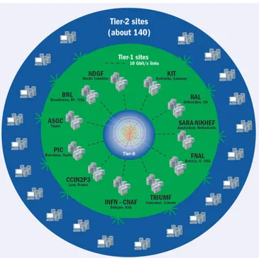
As stated previously the computing centres are organised in four Tier levels (see Figure 2.4):

• Tier-0 is deployed in two locations: CERN Data Centre in Geneva and Wigner Research Centre for Physics in Budapest. Tier-0 is responsible for the safe-keeping of the RAW data coming out of the detector, for first pass reconstruction, distri-bution of raw data and reconstruction output to the Tier-1s, and contributed to other tasks like data reprocessing.

• Tier-1 these are 13 computer centres with sufficient storage capacity but only 2 of them serve the needs of just one LHC experiment, all the others support more than one LHC experiment. Tier-1s operate a safe-keeping of a proportional share of RAW and RECO data, large-scale reporcessing and safe-keeping of corresponding output, data distribution to Tier-2s and sake-keeping of a share of simulated data produces at these Tier-2s.

• Tier-2 there are about 160 Tier-2s in LHC, usually not CERN-based such as uni-versities or scientific institutes. They provide CPU and storage for processing, both Monte Carlo productions and data analysis, with a balanced share among the two -but they are the primary resource for data analysis in the most experiments. They

(20)

Figure 2.4: Graphical representation of WLCG Tier levels.

handle analysis requirements and proportional share of simulated data productiona and reconstruction but do not have tape archiving.

• Tier-3 is a local computing resources for the users which can consists of local computer clusters or even just an individual PC. There is no formal engagement between WLCG and Tier-3 resources.

2.2.2 CMS Computing Model

The CMS project faces challenges not only in terms of the detector operation and the physics program, but also in terms of the data handing on computing resources. Most CMS collaborators are not CERN-based, and have access to significant non-CERN re-sources; therefore, the CMS computing environment [36] is based upon Grid middleware, with the common Grid services at centres defined and managed through the WLCG as explained beofore. Then, this computational infrastructure is intended to be available to CMS collaborators wherever they are. Basically a system of this kind must fulfill those needs:

• The analysis of a very large dataset requires a system of large scale, with an efficent approach to data reduction and patter recognition.

(21)

• Highly flexibility to make easy access to any data within the lifetime of the exper-iment. It must supports a wide variety of data processing tasks.

• A primary characteristic should be the manageability in its functionalities (i.e. computing operation and software thing)

Key components of the computing system [37] include:

• An event data model and correspondig application framework; • Distributed database system;

• A set of computing services;

• Underlying generic Grid services giving access to distributed computing resources; • Computer centres, managing and providing access to storage and CPU at local

level.

The disign challenges have been addressed through construction of a modular sys-tem of loosely coupled components with well-defined interfaces, and with emphasis on scalability to very large event samples.

The CMS application sofware must perform a variety of event processing, selection and analysis tasks, both online and offline. The central unit of the CMS data is the Event, which corresponds to a single bunch crossing; subsequent events with constant instantaneous luminosity form the Lumisections, and several Lumisections form the Run. Events from Runs are arranged into Datasets. Some data formats, with respect to their properties, are based on the Event: RAW digitised data, reconstructed produtc etc. The Event also contains information describing the origin of the RAW data and the provenance of derived data. The latter information allows users to unambiguously identify how each event contributing to a final analysis was produced; it includes a record of the software configuration and conditions/calibration setup used to produce each new data product. Events are physically stored as persistent ROOT files.

CMS makes use of several formats with different levels of detail of the information contained. The process of data reduction and transformation among formats takes place in several steps, usually is carried out at different computer centres.

RAW

RAW events contain the full recorded informations from the detector, plus a record of other metadata. RAW data is accepted into the offline system at the HLT output rate, and extension of the RAW data format is used to store the output of CMS Monte Carto simulation tools. This data type is permanently archived in safe storage and oc-cupies roughly 1.5MB/event. The RAW data are classified by the online system into

(22)

CMS data tier Size per event (MB) RAW Data 0.9 MiniAOD Data 0.032 RECO Data 2.2 AOD Data 0.370 RAW MC 1.5 MiniAOD MC 0.380 RECO MC 2.4 AOD MC 0.41

Table 2.1: Size of selected CMS data tiers, for Data and MC, at expected average PU 35.

several distinct primary datasets. This classification has several advantages such as the possibility of assigning priorities to data reconstruction and transfer. CMS will also define some flexible ”express streams” used for prompt calibration and rapid access to interesting or peculiar events.

RECO

Reconstructed (RECO) data are produced by applying several levels of patter recog-nition and compression algorithms to the RAW data. RECO data contains objects created by event reconstruction that is the most CPU-intensive activity in the CMS data processing chain and is made by mainly four steps:

1. Detector-specific processing (data decoding, application of detector calibration con-stants and objects are reconstructed).

2. Tracking (include reconstruction of global track from hits in the silicon and muon detectors).

3. Vertexing (reconstruction of primary and secondary vertex candidates)

4. Particle identification (produces the standard physics object which is most match-ing with physics analyses).

The RECO are not permanent in fact they can be recalculated when newer calibra-tions and better software are available. RECO events contain both the low level physics objects as hits, clusters etc and the high level objects such jets, muons, electrons etc. Moreover there is a direct connection between high and low level objects that avoids duplication of information. RECO events occupy roughly 0.5MB/event.

(23)

AOD

Analysis Object Data (AOD) is the compact analysis format, designed to be relatively small in size thus allowing large data samples in such format to be hosted in many computing centres. AOD events contain high-level physics objects, and additional infor-mation to allow kinematic refitting. AOD data are produced by filtering RECO data, either in bulk production or in a skimming process which may also filter a primary dataset into several analysis datasets.

AODSIM

AODSIM events are produced through Monte Carlo methods. They contain high-level information and are used for physics analyses.

MiniAOD

MiniAOD is a data tier of CMS data introduced in Spring 2014 to serve the needs of the mainstream physics analyses while keeping a small event size (30-50 kb/Event). The main contents of the MiniAOD are: high-level physics objects with detailed information; the full list of particles reconstructed by the ParticleFlow; trigger information, MiniAOD contains the trigger bits associated to all paths; plus there are objects reconstructed at L1 and the L1 global trigger summary [38].

In addition to event data, there is a variety of Non-Event Data, that is required in order to interpret and reconstruct events. CMS uses 4 types of Non-Event data: construc-tion data, equipment management data, configuraconstruc-tion and condiconstruc-tions data. Non-Event data are held in central Oracle databases, for access by online and offline applications. Conditions data access at remote sites take place via FroNTier system [39] which uses a distributed network of cache http proxy servers.

Within the CMS Computing Model 2 main sectors can be identified: the CMS Data Management System, focussing on access and storage aspects, and the CMS Workload Management System focussing on jobs flux handling. The detailed description of all the details of both sectors goes beyond the scope of this thesis. On the other hand, some aspects are important to set the context for the next chapters, so a brief and not exhaus-tive description is provided in the following.

(24)

2.2.3 Data and Workflow management

The CMS data management sector covers the cataloguing or alternative solutions to track the location of physical files on site storage systems, the transfer of files across sites, the aspects of data access, etc. The information about which data exists is offered by the CMS Dataset Bookkeping System. The Data Bookkeping Service [41] provides access to a catalogue of all event data, both from Monte Carlo data and collisions data, and it records the files metadata including its processing derivation (i.e. with the in-formation in the catalogue it is possible to track back to the original RAW data or Monte Carlo generation). The data managed by DBS are not actually data but point-ers to physical data organised by other parts of CMS data management system. The dataset replication system, i.e. static data placement, is implemented by the PhEDEx system. The PhEDEx (Physics Experiment Data Export) [42] is a reliable and scalable dataset replication system targeted to serve large scale data transfer needs across Grids. PhEDEx provides a centralized system for making global data movement decisions and a realtime view of the global CMS data transfer state. PhEDEx is composed of a seried of autonomous, persistent processes, called agents, which share information about replica and transfer state through a database. Agents are very specialized, e.g. there are agents for download, for tape migrations, etc. Recently, Dynamic Data Management features have been added to dynamically delete unused data replicas and further replicate heavily accesses ones.

The workload management sector of the CMS Computing Model is focused on the solu-tions needed to be able to process and analyze data at Grid sites through preparation and submission of jobs to distributed resources and recovery of job output. A standard job submission process performs the necessary environment set-up, executes a CMSSW [43] application on local resources, arranges for any data to be made accessible via Grid data management tools, allows to recover the processing output, and provides logging information for the entire process. Over the past years, the architecture has moved to pilots and CMS relies on the Glide-InWMS for most pre-processing functions. At the application level depending on which is the nature of the processing jobs, different ar-chitectural needs arise and CMS implemented two separate systems: WMAgent [44] for centralize production processing, and CRAB for distributed Grid analysis. The descrip-tion of both fo beyond the scope of this thesis, in particular the former. The latter is quoted in the following, so it is briefly introduced below.

The CRAB [45][46] is a CMS dedicated tool for workflow management for analysis jobs. Its main feature is allowing users to submit jobs to a remote computing element which can access to data previously transferred to a close storage element. Its main functions are: interfacing with the user environment, data-discovery/location services, job execution and monitoring, output recovery and out data transfer to final destination (the Asynchronous StageOut component). Via a simple configuration file, a user can thus

(25)

access data available on remote sites as easily as he can access local data. A client-server architecture allows the jobs to be not directly submitted to the Grid byt to a dedicated CRAB server, which, in turn, handles the job on the behalf of the user, interacting with the Grid services. This allows to insulate all retrials and resubmissions, thus simplifying the user experience.

The Data Bookkeeping Service provides access to a catalogue of all event data from Monte Carlo and Detector sources and records the files and their processing derivation. With the information in the catalogue it is possible to track back to the original RAW data or Monte Carlo generation. Data files are mapped to File Blocks that pile related files for data placement purpose, their location is tracked by DBS too. The system is built as a multi-tier web application, and is used for distributed analysis, production data processing activitied, and associated with the data location in PhEDEx. The data managed by DBS are not actually data but pointers to physical data organised by other parts of CMS data management system. Typical uses of DBS include MC generation, detector data, large scale production processing and user data analysis. The data have to be transfed among several service levels, this operation is took over by PhEDEx (Physics Experiment Data Export). This project is a source for large scale data transfers across the Grid. PhEDEx provides a centralized system for making global data movement decisions and a realtime view of the global CMS data transfer state. Many of low level tasks (large-scale data replication, tape migration...) for CMS are automated. PhEDEx is composed of a seried of autonomous, persisten processes, in PhEDEx terms agents. The agents task is to share information about replica and transfer state through a database.

2.3 The CMS dataset popularity

The data management is a very hard challenge, especially when dealing with huge amount of data; one take account of limited storage capacity, not all data can be hold forever. The CMS experiment has collaborations all around the world which submit everyday about 200000 jobs, it entails considerable application of Grid workload and resources to manage corresponding data. Thus, a big goal is to create a compunting model for the optimisation of usage and storage availability through automated procedures. The main purpose is to make a transition from static data placement to dynamic one. CMS developed this project, the CMS Popularity Service, learning from ATLAS similar expe-rience. A useful brand new concept is introduced the “data popularity”. A early topic was about the PhEDEx Service [47] whose feature is to create and distribute the files copies at each site; then, many users may keep access to the same files, but for the storage space sake how is it possible to decide which copies are useful and which are not? In this task the “data popularity” concept occurs; it is a misurable parameter able to quantify the interest of the users analytics for data exiting from MC simulation or data samples; monitoring the number of access and upshot to files by users’ job. The CMS Popularity

(26)

Service tracks the time evolution of : dataset name, number of access, success or failure of data access, CPU hours, number of each users that execute the access. This system is still in progress, currently the informations collected are used to trigger ad-hoc can-cellation of least used replicas and trigger ad-hoc replication of which one is considered most popular. A long term goal is to improve this model with the target to be adaptive and able to predict future behaviours of the CMS systems from the monitoration of their performances in the past.

Data treatment

The CMS experiment during both the run1 and run2 has acquired plenty of data; the data used for analysis go under transformation in format and reduction in content (only essential informations are taken). The computing process goes as follow: the collisions data are streamed to HLT (High Level Trigger) and then organized into trigger streams. They are collected at the Tier-0 center and allocated to CMS Analysis facility (CAF) at CERN and Tier-1s. Later, a portion of those data are moved to Tier-2s for simu-lation process (MC generation). The final step are analysis tasks at Tier-3s. All these data, as above, are replicated in multiple copies (PhEDEx) and accessed by analysis groups using the WLCG services; in CMS is mostly used CRAB. The data are logically organized into run,files, blocks, and dataset. Part of those data (see below) refers to operations themselves, monitoring data, machine logs etc. but they are rarely accessed and analysed, because more focus is given to near-time debugging purposes than a study of time trend. In addition those data result in a dataset that needs a data validation and cleaning process before being suitable.

Type of data

There is another type of data and metadata concerning the performances of the comput-ing operations, this is an heterogeneous ensemble of non-physics data known as structured and unstructured. In common jargon the structured data refers to information with high degree of organization; in CMS it is a collection of information about CMS Computing activities and are suitable via CMS data service APIs (Application Program Interface). For example the already quoted PhEDEx transfer management database is a source of structured data, and the DBS system (the CMS source for physics meta-data); fur-ther examples are: the Popularity Database for dataset user access information; SiteDB collects information about pledges at WLCG sites, deployed resources; the CERN Dash-board that is a big repository of details on Grid jobs etc.. The unstructured data type on the other hand, generaly doesn’t have a definite location because cannot be easily stored in a database, in despite of this difficulty usually it is rich in content; unstructured data for example are HyperNews forums, CMS twikies etc. Alongside there is also the semi structured data which is a kind of information not located in a relational database but

(27)

at the same time it can be analyzed easly, follows a sort of scheme in organization and can be stored in a database; it can be found from CMS web logs, calendar systems. Relevance and application of data popularity

The data popularity is a metric of interest for efficient data placement strategies based on users’ activities. The easiest way to understand end-users’ interest is to invesigate the datasets popularity, infact these latter are usually used as principal unit in data analysis process and they are also the final product of this chain. So, can be stated that the knowledge about the nature of CMS dataset popularity aims to optimize the computing model and reduce its operational cost. A question arises as of which is the “best” way to define the popularity: in practice, any definition will work provided that its appli-cation allows to produce predictions of practical use. To build a proper definition, the popularity DB provides a quite wide range of metrics: the number of accesses to a given dataset, the numer of users/day recorded in accessing a dataset, the total number of CPU hours spent accessing a given dataset, along with normalized values of those attributes over full number of datasets. Depending on the specific kind of usage of the popularity data, definitions may change and require work to define the most adequate one for the objective of the study.

(28)

Chapter 3 Studies of CMS data access patterns

First of all it is usefull to explain how the collected data are arranged and organized, and general feature of the plots we will present and comment.

In this work we use popularity data from 2014 to 2016. For every year, the “data keeping period” (the time of the year in which we collect and keep the data for further analysis) ends in March, June, September and December; so, data is collected and analyzed every quarter.

Subsequentely, data is analyzed into three categories that we call “time windows”: 3M, 6M, 12M. These classes refer to 3, 6, and 12 months in the past starting from a given month and year. Finally, data are sorted by number of accesses. As a final outcome, we are interested in the volume of data, both accessed and non-accessed, within each time window in the past starting from the end of a given data keeping period. The goal is to use this general information related to the data volume hosted on Grid storage to study the CMS data accesses and try to extract particular usage patterns.

In the following, several graphs will be shown and explained. The format of some of those plots is the same required to be shown at the WLCG Computing Resources Scrutiny Group, a formal body whose task is to inform the decisions of the Computing Resources Review Board (C-RRB) for the LHC experiments. These plots - that will be quickly referred to as ”scrutiny plots” in the following - show the fraction of data volume that was accessed 0 times, 1 time, or more. In particular, the data volume with 0 accesses is divided in two bins, the so-called “0-old” bin and the so-called “0” bin: they all contain volumes that recorded 0 accesses, but the former groups the existing data older than the given time window, while the latter refers to new data produced (thus, newer than each given time window). Their utility will become more clear in the following sections.

(29)

3.1 Global view

Given the premises as in the previous section, in this section the focus is the study of the patterns of CMS data accesses with no particular breakdown into any specific data type or any specific WLCH Tier, i.e. we will consider access to CMS data to all data types interesting for analysis on all Tiers where they may reside. A global view is interesting as it allows to get a first overall picture of how the CMS storage is actually used in analysis.

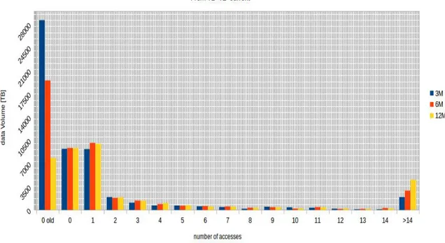
Figure 3.1: The scrutiny plot (see text for explanation) showing the total data vol-ume (AOD, AODSIM, MiniAOD, RECO) accessed from Tier-1 and Tier-2 sites as from September 2016, subdivided by time window and number of accesses.

As initial example we consider the current data keeping period (September 2016). In Figure 3.1 a scrutiny plot is displayed, and it allows to perform a few considerations. First, we can see that the only bins of interest are 0 old, 0, 1 and > 14, the orthers being much lower is size, and more regular, hence less relevant. The yellow bar, which refers to 12 months in the past (from September 2016), provides this information: if we look back from September 2016, we see that there are about 8PB older than 12 months and never used; about 10PB younger than 12 months that in these 12 months have recorded zero

(30)

accesses; more than 10PB of data with only 1 access in the last 12 months; the rest is accessed more than 1 time in the last 12 months, peaking at about 4 PB accessed many times (> 14 in the standard scrutiny plot). A quick comparison with the other time win-dows is instructive. We can see that tightening the time window, the > 14 bin decreases, ad this is explainable because over 12 months there is more probability for this data to have been accessed than there is over only 6 or 3 months in the past. In particular, the 12 months window will tend to be very inclusive (sort of “catch all”) whereas the 3 months will tend to be more exclusive (sort of “tooshort time in the oast to reflect actual analysis interest”). This leads us to first preliminary but interesting observation, that we will also apply in the rest of the thesis: among the considered three time windows, the 6 months time windows is the most realistic estimate of what really happes in terms of data access. Back on Figure 3.1, if we look at the 0-old bin difference between the 12 months time window and the 6 months time window, the latter is twice larger: the more you look into the past, the smaller the 0-old bin will become, but it is still of considerable size. This is an indication that regardless the old data deletions from disks that CMS performs, there is still sizeable fraction of “old data” that remains on disk and is unaccessed. This information has a value when analyzed in terms of its dependence with time (see in the following sections).

Back on Figure 3.1, if we look at the 1-bin, we observe that its size in the 3, 6, 12 months time window is roughly 10PB (little less in 3M). A first observation is that being this bin much higher than most other bins apart from the 0-bins, it shows that CMS analysis teams tends to have on average just one submission pass over interesting data, from which they produce derived data which they further analyse (and those accesses are not counted/showed in this kind of plot). A second observation is that the size of the 1 bin and the 0-new bin is comparable in each time window, implying that it may be concluded that the fraction of data younger than any selected time window have a 50% chance of being accessed once or a 50% chance of being left unaccessed in that time window.

At this point, it can be instructive to deviate from the standard scrutiny plot format and face the problem in a different way: display, in different time windows in the past from a given time (a moving reference, of course), only the datasets that have been accessed at least once (i.e. > 1 bins altogether) and the datasets that have never been accessed (i.e. 0-old and 0 bins altogether). One example is shown in Figure 3.2 where the observables above are shown for accesses in the last 3, 6, 12 months and at all Tier levels of interest (Tier-1 and Tier-2) for all data types of interest, i.e. AOD, AODSIM, MiniAOD and RECO. This allows to perform a few interesting considerations.

(31)

Figure 3.2: Same data as from Fig. 3.1, but displayed with aggregate bins (see text for explanation). The yellow line displays the sum of the red and blue bins, which show the non-accessed and accessed data volumes respectively, for each of the three considered time windows in the past, starting from September 2016.

(32)

time window should correspond to the total existing data volume on disk in that time window - as there is no data that can be in a condition that is not one of these two mutually exclusive categories. While is true inside a specific time window, this may well change from one time window to another: the total data volume is impacted by data proliferation as well as data deletion, and both happen at different time windows in a largely unpredictable manner (i.e. in ways related to the CMS experiment activities and needs). A pragmatic approach to evaluate how the situation is evolving could be to measure the total data volume in each time window (the yellow line in Figure 3.2) and see how it evolves over time (i.e. from the 12M time window, through the intermediate 6M time window, to the 3M time window - note, going from the right-hand side to the left-hand side in Figure 3.2): if the yellow line shows an increasing trend, it means that over time data was created more than deleted, whereas if it decreases, data was deleted more than created. This information is useful because then one can check the fraction of accessed data volume, knowing the trend in the total existing data volume, and thus being in a condition to draw some conclusions.

To explore this, more insight is needed and we must go beyond the general overview across all data types and WLCG Tiers, which was the focus of this section. An analysis of the patterns we observe can hence be attempted by considering that the popularity data has been collected for various data types (AOD, AODSIM, MINIAOD, RECO) and for accesses at Tier-1 sites and Tier-2 sites separately. We are in good position then to explore data access patterns we observe, according to different views, and this is explored in the next sections.

3.2 Evolution with time

In this section, the focus is the study of the patterns of CMS data accesses with no particular breakdown into data type or WLCG Tiers, i.e. the “global view” as from the previous section, but studying how it evolves over time. This is done by studying sliding time windows, i.e. 3, 6, 12 months in the past starting from the present, from 3 months ago, from 6 months ago, etc and going 2 years into the past. The key point of the study of time evolution aspects is that we can envision the whole set of data as a flux and we are interested in its ensemble behavior, namely we would like to verify is observed patterns would stay unvaried or not, and what this would imply.

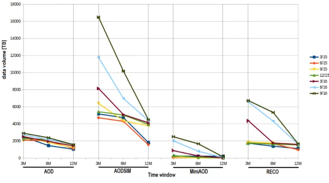
Unlike the plots in the previous section Figure 3.3 represents the evolution with time of the global view: now we focus on how bins contents (that is a ensemble of AOD, AODSIM, MiniAOD, RECO data tiers) is evolving per data keeping period, highlighting the time windows of 3, 6, 12 months in the past. Despite the plot contains plenty of details and it is hard to read, global behaviours can be extracted from it and they help

(33)

in assessing how the storage management health is currently in CMS. All the bins as from the previous section are displayed in different colors, but we discard all bins from 2 accesses to 14 accesses, as their flatness relveals a quite regular activity which is not particularly relevant in the current study. We emphasise only the following bins: 0-old, 0, 1 and > 14. Let’s re-state the importance of each bin in terms of what it is intended to display, so we may settles on what an “expected” behaviour over time would be, and then check with the data if we indeed observe this expected behaviour or deviations from it.

The 0 old bin, for the reasons we already stated in the previous section, can be as-sumed as a parameter that tells how good CMS is in cleaning-up relatively old data that still occupy disk space (e.g. LHC Run-1 data fall for sure in this category). The 0 bin can be conceived as a parameter that tells how good CMS is in making sure that the data collected and produced relatively recently are indeed accessed from disks (e.g. data just produced may well not be accessed yet, but data produced some time ago should have been recorded some accesses). Quite another this is the bin 1, as it represents the data volume in each given time window with just one access (and in many case the number 1, as discussed earlier, is not representative of the real activity over the dataset). In an ideal world a perfect placement strategy must aim to avoid the 0-old bin (i.e “keep disks clean from old unaccessed data”), to reduce the 0 bin to a decently low level, and to increase ad needed the size of the bins from 1 to N. This situation, if observed in this kind of plots, would reflect a more efficient use of the Grid storage, even in the constant presence of newer data being recorded and accessed.

(34)

Figure 3.3: Trend of number of accesses per data keeping periods, time windows and data tier.

(35)

With these premises, from Figure 3.3 we can speculate about some aspects:

1. A first consideration concerns the AOD data type. In general looking inside each time window in the past from a given period we can state that the oscillation be-tween non-accessed and accessed data volume are well balanced. Looking through the whole set we can notice that bin > 14 is decreasing and bin 0-old is increasing between June and September 2016. In fact at least 75% of analysis operations can be performed on MiniAOD but there is still a small part 25% of the analyses that have not migrated and still use AOD. We know that the MiniAOD format has been introduced in CMS in late 2014, and indeed one sees aforementioned effects of their presence in late 2015: for AOD during March-December 2015 there are more accessed data than non-accessed ones. Moreover, in this same period, the orange line (that rapresents the 0 bin) is quite flat: this means that most recent data used to be accessed relatively quickly in unpredictable distributed analysis; then, in late 2015 the behaviour slowly changes and the accesses started to be apparently more slowly. A first qualitative example, the 0-old and also the 0 started to grow more slowly. A second quantitative example, considering the 12 months time window in March 2015 and the 3 months time window in September 2016, in two years, the data volume of the > 14bin is decreased of 69%. These observations on AOD will be confirmed by the observations on MiniAOD (see bullet 3 below).

2. A second, indipendent consideration is about the situation of AODSIM. The fig-ure shos that this is evidently becoming more and more critical over time. The bins 0-old, 0 and 1 are increasing considerably over time, while the > 14 bin is constant. The AODSIM data tier has simulated event content produced by Monte Carlo simulation, and it is known that in CMS lately its amount (and access) has increased. In this case the 0-old bin exceeds 16PB during the last 3 months since September 2016, but such data volume is consistent with the fact that there has been an ingent production activity as can also be inferred by the 0 bin increasing trend (i.e. data produced recently and not yet accessed). However, as shown by the plot, the overall CMS space management has gradually worsened (e.g.see the situation during the 3 month in the past from March 2015 when the non-accessed data volume was already about 5PB despite of 0 bin and 1 bin which were about 0.5PB and 1PB respectively). We also notice that the 1 bin has (in the case of AODSIM) more entries than other bins in many time windows over the last 2 years: it may look quite odd that data of interest are really used just one time, but this may just be an effect of the fact that this data is used as initial step by analysts and then they use only the outcome, in agreement with what stated in the previous section.

3. The MiniAOD data format, introduced since late 2014, shows a very interesting evolutive path: in March 2015 there were mostly 0 old and then from December

(36)

2015 till now we can see an evident ramp-up. This confirms what stated in the first point of the AOD data type. This data tier is growing steadly in terms of accessed since its birth, and in a quite healthy manner: of course there are older data on disk being accessed less, but the volume of data accessed is always larger than the volume of data non-accessed. In a general trend, it is quite easy to note that MiniAOD have reached during Semptember 2016 a volume comparable to AODs. One should also remember that the MiniAOD size is a factor 10x smaller than the AOD, so e.g. a MiniAOD data file mistakenly left (not cancelled) on disk is “wasting” 10 times less space than a similar action done for AODs. Additionally, the MiniAOD data type in this plot must be taked ad a MiniAOD*, i.e. it groups MiniAOD and MiniAODSIM data format, so in principe we should be comparing MiniAOD here with AOD and AODSIM summed up. Now it is clear th impact of MiniAOD on the CMS storage worldwide: the CMS analysis teams (at leats at the 75% level) can perform their usual analysis routine with much less storage space needed, and growing on the Grid in a much more healthy manner.

4. On a last point, the RECO data format is also displayed. This data type is crucial for some dedicated studies but it is of limited relevance to the CMS Grid analysis community, getting decommissioned soon (i.e. same content in AOD and in most cases also in MiniAOD). As displayes in Figure 4.7, early in 2016 the volume of old non-accessed data (0-old bin) started to raise much more than recent non-accessed data (0 bin): RECOs were indeed prodced less, and most of the old ones were kept of disk for last access needs before speeding up with the decommissioning. Becoming soon obsolete, this format is less relevant in this thesis, despite being included as this format is still one of those accessed by CMS analysis jobs on the Grid.

From the observation so far, the role of the information displayed in the 0-old bin seem one of the most relevant. Most (almost all) of the conclusions in this sections can be inferred by looking at the 0-old bin only (e.g. looking at the dark blue line in Figure 3.3). For this reason, it is interesting to transform the visualization as in Figure 3.3 into an evolution with time of the 0-old bin only, and display it in a different way. In Figure 3.4, for each type, each coloured line shows the situation at a specific moment in time (and the 3 points on each line show how this situation changes if one looks 3, 6 , 12 months in the past): in this way, one can observe how the situation indeed changed over time by looking at lines of different colour, and it is easier to catch a peculiar pattern in data and found evidences of what stated above.

Firstly, one can start from the AOD data type: the trend through the years is always monotone increasing going from 12 months in the past to 3 months in the past. In prin-ciple, we have also evidence of regular accesses through the year (e.g. correlation with

(37)

conferences and holidays), and we could draw more hypothesis about working periods, etc.

Secondly, one can look at the AODSIM data type. By taking e.g. each 3M time windows, a worsening is seen: obviously in this plot the bin 0-new and 1 are not shown by choice, but the behaviour over time of the 0-old alone well supports the hypothesis of CMS space management getting progressively worse as and effect of the presence of this (AODSIM) data tier.

Thirdly, the MiniAOD trend - at least in the periods when it existed already - can be seen indeed ad the motst healthy: no inflation of the 0-old bin is observed over recent times, despite a considerable grow in the MiniAOD data volume over last couple of years. For the reasons outlined in a previous paragraph, we do not further investigate the details of the RECO access patterns.

(38)

3.3 Data types view: RECO, AOD, AODSIM, MiniAOD

In this section, the focus is the study of the patterns of CMS data accessed with break-down into the different analysis data tiers: RECO, AOD, AODSIM, MiniAOD. We start from a general study of how and how much a single data tier is used; then we consider different combinations of main parameters and their outcome; finally some considerations deriving from the study of time window. Again, the data used are from both Tier-1 and Tier-2, with no distinction between them.

As a reminder, each step in the simulation and recostruction chain gives information about events which are stored into what we call a “data tier”. A data tier may be com-posed by multiple data formats, then a dataset may consist of multiple data tiers. In the following some considerations about different aspects of each data tier are discussed. One of the reasons for this study is to properly disentangle e.g. the contribution of AOD and AODSIM separately.

First of all, we can make an a-priori consideration about time windows: ideally, data access patterns should reflect the activity of CMS analysts, which on a global scale does not react so quickly after data is available, because realistically few weeks are needed for changes to be reflected on CMS-wide average behaviours. This means that, translating it in terms of time windows, a 3 months window might be simple too short (we got a superposition between non-accessed new and old data); a 12 months window might be too large (it is easy to find more data accessed during long periods); a 6 months window is a good compromise. Moreover it is on average the time window between two major series of conferences, speaking of ”Winter” conferences and ”Summer” conferences. This latter point will be clarified in the next section. At the time being we consider a 6 months time window as the most significant for the considerations in this section.

(39)

Figure 3.5: Data volume accessed in 3M, 6M, 12M time windows in the past starting from June 2016. See text for detailed explanations.

In the following paragraphs, we will focus on the one data tier at a time, and discuss it throughly.

AOD

As discussed previous, and also shown in Figure 3.5, the regularity of AOD total volume (i.e. sum of 0 accesses and > 0 accesses volumes) in a fixed period is evident: there is a decrement of 0.005% in total volume going from 12 months to 3 months in the past, hence totally negligible. The previous consideration about the adequateness of the 6 months time window applied to the AOD case: as we can see in Figure 3.5, during this period the analysts have accessed, over a total of roughly 6PB, about 60% of the data volume and only about 40% has remained non-accessed (whereas the 12 months window would be too optimistic i.e. 2/3 and 1/3, and the 3 months window would not yield yet any useful interpretation of the data).

On Figure 3.6 we describe the 6 months behaviours of the AOD data tier in its time evolution. More (i.e. also 3M and 12M) can be found in Appendix C, anyway in general they are consistent in showing the time evolution pattern of total accessed and non-accessed data volume for AODs: over time (x-axis), looking at 6 months in the past (as