2020-05-29T07:24:58Z
Acceptance in OA@INAF
A 1.9 Earth Radius Rocky Planet and the Discovery of a Non-transiting Planet in
the Kepler-20 System
Title
Buchhave, Lars A.; Dressing, Courtney D.; Dumusque, Xavier; Rice, Ken;
Vanderburg, Andrew; et al.
Authors
10.3847/0004-6256/152/6/160
DOI
http://hdl.handle.net/20.500.12386/25285
Handle
THE ASTRONOMICAL JOURNAL
Journal
152
A 1.9 EARTH RADIUS ROCKY PLANET AND THE DISCOVERY OF A NON-TRANSITING
PLANET IN THE KEPLER-20 SYSTEM
*Lars A. Buchhave1, Courtney D. Dressing2,19, Xavier Dumusque3, Ken Rice4, Andrew Vanderburg5, Annelies Mortier6, Mercedes Lopez-Morales5, Eric Lopez4, Mia S. Lundkvist7,8, Hans Kjeldsen7, Laura Affer9,
Aldo S. Bonomo10, David Charbonneau5, Andrew Collier Cameron6, Rosario Cosentino11, Pedro Figueira12, Aldo F. M. Fiorenzano11, Avet Harutyunyan11, Raphaëlle D. Haywood5, John Asher Johnson5, David W. Latham5,
Christophe Lovis3, Luca Malavolta13,14, Michel Mayor3, Giusi Micela9, Emilio Molinari11,15, Fatemeh Motalebi3, Valerio Nascimbeni13, Francesco Pepe3, David F. Phillips5, Giampaolo Piotto13,14, Don Pollacco16, Didier Queloz3,17,
Dimitar Sasselov5, Damien Ségransan3, Alessandro Sozzetti10, Stéphane Udry3, and Chris Watson18
1
Centre for Star and Planet Formation, Natural History Museum of Denmark & Niels Bohr Institute, University of Copenhagen, Øster Voldgade 5-7, DK-1350 Copenhagen K, Denmark;[email protected]
2
Division of Geological and Planetary Sciences, California Institute of Technology, Pasadena, CA 91125, USA
3Observatoire Astronomique de l’Université de Genève, 51 ch. des Maillettes, 1290 Versoix, Switzerland 4
SUPA, Institute for Astronomy, University of Edinburgh, Royal Observatory, Blackford Hill, Edinburgh, EH93HJ, UK
5
Harvard-Smithsonian Center for Astrophysics, 60 Garden Street, Cambridge, Massachusetts 02138, USA
6
SUPA, School of Physics & Astronomy, University of St. Andrews, North Haugh, St. Andrews Fife, KY16 9SS, UK
7
Stellar Astrophysics Centre, Department of Physics and Astronomy, Aarhus University, Ny Munkegade 120, DK-8000, Aarhus C, Denmark
8
Zentrum fr Astronomie der Universitt Heidelberg, Landessternwarte, Knigstuhl 12, D-69117 Heidelberg, Germany
9
INAF—Osservatorio Astronomico di Palermo, Piazza del Parlamento 1, I-90124 Palermo, Italy
10
INAF—Osservatorio Astrofisico di Torino, via Osservatorio 20, I-10025 Pino Torinese, Italy
11
INAF—Fundación Galileo Galilei, Rambla José Ana Fernandez Pérez 7, E-38712 Breña Baja, Spain
12
Instituto de Astrofísica e Ciências do Espaço, Universidade do Porto, CAUP, Rua das Estrelas, PT4150-762 Porto, Portugal
13
Dipartimento di Fisica e Astronomia“Galileo Galilei”, Universita’di Padova, Vicolo dell’Osservatorio 3, I-35122 Padova, Italy
14INAF—Osservatorio Astronomico di Padova, Vicolo dell’Osservatorio 5, I-35122 Padova, Italy 15
INAF—IASF Milano, via Bassini 15, I-20133, Milano, Italy
16
Department of Physics, University of Warwick, Gibbet Hill Road, Coventry CV4 7AL, UK
17
Cavendish Laboratory, J J Thomson Avenue, Cambridge CB3 0HE, UK
18
Astrophysics Research Centre, School of Mathematics and Physics, Queen’s University Belfast, Belfast BT7 1NN, UK Received 2016 June 13; revised 2016 August 23; accepted 2016 August 24; published 2016 November 11
ABSTRACT
Kepler-20 is a solar-type star(V = 12.5) hosting a compact system of five transiting planets, all packed within the orbital distance of Mercury in our own solar system. A transition from rocky to gaseous planets with a planetary transition radius of ∼1.6RÅ has recently been proposed by several articles in the literature. Kepler-20b (Rp∼1.9RÅ) has a size beyond this transition radius; however, previous mass measurements were not sufficiently
precise to allow definite conclusions to be drawn regarding its composition. We present new mass measurements of three of the planets in the Kepler-20 system that are facilitated by 104 radial velocity measurements from the HARPS-N spectrograph and 30 archival Keck/HIRES observations, as well as an updated photometric analysis of the Kepler data and an asteroseismic analysis of the host star (M=0.9480.051M and
R =0.9640.018R). Kepler-20b is a 1.868-+0.0340.066RÅ planet in a 3.7 day period with a mass of
-+
9.70 1.441.41MÅ, resulting in a mean density of 8.2-+1.31.5g cm-3, indicating a rocky composition with an
iron-to-silicate ratio consistent with that of the Earth. This makes Kepler-20b the most massive planet with a rocky composition found to date. Furthermore, we report the discovery of an additional non-transiting planet with a minimum mass of19.96-+3.61
3.08 Å
M and an orbital period of∼34 days in the gap between Kepler-20f (P∼11 days) and Kepler-20d(P∼78 days).
Key words: planetary systems– planets and satellites: composition – stars: individual – techniques: radial velocities Supporting material: machine-readable table
1. INTRODUCTION
With the discovery of thousands of small transiting exoplanets by dedicated space-based missions like NASA’s Kepler mission(Batalha et al.2013) and ESA’s CoRoT mission
(Auvergne et al. 2009), a new class of small planets has
emerged. In contrast to the hot-Jupiters, these small planets
(<4RÅ) are astonishingly common in our Galaxy (Howard
et al. 2012; Dressing & Charbonneau 2013, 2015; Petigura et al.2013; Burke et al.2015). We now know that the majority
of stars harbor small exoplanets and that nearly two-thirds of the planets discovered by Kepler range in size between 1 and 4RÅ. This unexpected population of super-Earths and
sub-Neptunes—larger than Earth but smaller than Neptune (3.9RÅ)
—is completely absent in our own solar system, which furthermore lacks planets with orbital periods shorter than the 88-day orbit of Mercury.
Although we know of thousands of these small transiting exoplanets, only a few of these currently have precise mass
© 2016. The American Astronomical Society. All rights reserved.
* Based on observations made with the Italian Telescopio Nazionale Galileo (TNG) operated on the island of La Palma by the Fundación Galileo Galilei of the INAF(Istituto Nazionale di Astrofísica) at the Spanish Observatorio del Roque de los Muchachos of the Instituto de Astrofísica de Canarias.
19
measurements (precision better than 20%) that could allow us to distinguish between different compositional models. Precise masses and resulting bulk densities are especially important for small planets, since a wide diversity of planet compositions are possible, including rocky terrestrial planets with compact atmospheres and rocky cores with significant fractions of volatiles, like water and methane, and/or extended hydrogen/ helium envelopes. A transition from rocky to gaseous planets has been proposed to occur at planetary radii of around 1.5–1.7RÅby a number of authors(e.g., Weiss & Marcy2014;
Rogers2015).
The Kepler-20 system is particularly interesting because Kepler-20b has a radius (Rp b, =1.868-+0.0340.066RÅ) beyond the
proposed transition to planets with a significant fraction of volatiles and is amenable to precise determination of its bulk density. Furthermore, the Kepler-20 system is intriguing in terms of its formation history, because of its compact nature and the size of the planets, which alternate between smaller and larger planets in the interior of the system.
Four of the transiting planets in the Kepler-20 system were first announced as candidate planets in Borucki et al. (2011).
Gautier et al. (2012) subsequently validated three of the
planets, including mass measurements of Kepler-20b
( = -+ Å Mp b, 8.7 2.2M 2.1 ) and Kepler-20c ( = -+ Å Mp c, 16.1 3.7M 3.3 ).
Later Fressin et al. (2012) validated two additional Earth-size
planets (Kepler-20e and f) increasing the total number of planets in the Kepler-20 system to five, all packed within the orbital distance of Mercury in our own solar system (see Figure 1 for a graphical presentation of the system architecture).
In this paper, we revisit the mass determination of the planets in the Kepler-20 system with the goal of improving the masses
and radii of the planets in order to allow us to discriminate between different compositional models. In particular, we attempt to resolve whether Kepler-20b has a rocky or gaseous composition, since the mass determination in Gautier et al. (2012) was not of sufficient precision to draw firm conclusions
regarding its composition. We have significantly increased the number of radial velocity(RV) measurements by adding 104 HARPS-N observations to the existing 30 HIRES measure-ments, allowing a more precise mass determination. Moreover, the new RV measurements allowed us to discover a non-transiting planet in the system situated in the gap between Kepler-20f and Kepler-20d, which we denote as Kepler-20g. Lastly, we performed an updated photometric analysis of the Kepler light curve using all the available data in conjunction with an asteroseismic analysis of the parameters of the host stars, yielding a significantly improved precision on the stellar radius and thus the radii of the planets.
2. OBSERVATIONS AND DATA REDUCTION We obtained 125 observations of Kepler-20(KOI-70, KIC 6850504, 2MASS J19104752+4220194) with the HARPS-N spectrograph on the 3.58m Telescopio Nazionale Galileo (TNG) located at Roque de Los Muchachos Observatory, La Palma, Spain(Cosentino et al.2012). HARPS-N is an updated
version of the original HARPS spectrograph on the 3.6m telescope at the European Southern Observatory on La Silla, Chile. HARPS-N is an ultra-stable fiber-fed high-resolution (R=115,000) spectrograph with an optical wavelength cover-age from 383 to 693 nm, designed specifically to provide precise radial velocities. The instrument has significantly improved our understanding of small transiting planets with Figure 1. Orbital configuration of the Kepler-20 system, where all the planets are packed within the orbital distance of Mercury. The orbital distances are to scale and the planet sizes are scaled to the correct size relative to each other, but have been increased significantly (The radius of Kepler-20g has been estimated using its mass and assuming a similar composition as Kepler-20c). The blue lines represent the planets with mass measurements.
several precise mass measurements of transiting planets(Pepe et al.2013; Bonomo et al.2014; Dumusque et al.2014; López-Morales et al. 2014; Dressing et al.2015; Gettel et al. 2016).
We obtained 61 and 64 observations of Kepler-20 in the 2014 and 2015 observing seasons, respectively(125 observations in total). We rejected 21 observations obtained under poor observing conditions where the internal error estimate exceeded 5m s-1leaving a total of 104 observations.
Kepler-20 has a mV= 12.5 and required 30 minute exposure times to build up an adequate signal-to-noise ratio(S/N). The average S/N per pixel of the observations at 550 nm is 30, yielding an average internal uncertainty estimate of 3.66m s-1.
The data were extracted and reduced with the standard HARPS-N pipeline. The extracted spectra were cross-corre-lated with a delta function mask based on the spectrum of a G2V star(Baranne et al.1996; Pepe et al.2002). The resulting
radial velocities and their 1σ errors are shows in Table1along with their weighted midtime of exposure in BJD UTC, and the activity indicators FWHM (full width at half maximum) and
¢
R
CaIIlog( HK), with respective uncertainties and S/N at
550 nm.
Gautier et al. (2012) obtained 30 spectra of Kepler-20
between 2009 August and 2011 June using the HIRES spectrometer on the Keck I 10 m telescope (Vogt et al. 1994). With a typical exposure time of 30–45 minutes
on a telescope with a light collecting power of almost a factor of 8 greater than that of the TNG, the average S/N per pixel is 120, yielding an average internal uncertainty of 3.04m s-1. If
the internal errors are taken at face value, the increase in S/N by 400% leads to a increase in RV precision of only 20% when compared to the HARPS-N RVs. In Section5, we calculate the average internal uncertainty, including an added jitter term for each instrument. The conclusion is that the average internal uncertainty of the HIRES RVs is 23% more precise than the HARPS-N RVs, despite the 400% higher S/N.
3. STELLAR PROPERTIES 3.1. Spectroscopy
Gautier et al.(2012) obtained stellar parameters for
Kepler-20 from two HIRES template spectra, without the iodine cell, that were analyzed using SME (Valenti & Piskunov 1996; Valenti & Fischer 2005), yielding Teff=5455±44 K,
=
g
log 4.40 0.10, [Fe H]=0.01±0.04, and vsini<
2km s-1. The Stellar Parameter Classification tool (SPC;
Buchhave et al.2012,2014) was also used to analyze spectra
from FIES, McDonald, and HIRES, yielding Teff=
5563±50 K, logg=4.520.10, [m H]=0.04±0.08,
and vsini=1.8±0.5km s-1, consistent with the SME
values, except for the effective temperature, which is 108 K higher.
We used SPC (Buchhave et al. 2012, 2014) to derive the
stellar parameters of the host star from the 125 high-resolution high S/N HARPS-N spectra (average S/N per pixel of 30). Since SPC does not require a very high S/N, we were able to utilize all the spectra for the analysis. We ran SPC with all parameters unconstrained and with the surface gravity constrained to the value determined from asteroseismology (logg=4.4460.01, see Section 3.2). The surface gravity
from the unconstrained SPC analysis,logg=4.500.10, is in close agreement with the value from asteroseismology. The unconstrained weighted mean of the SPC results from the individual spectra yielded: Teff=5532±50 K,logg =4.50
0.10, m H[ ]=0.08±0.08, and vsini<2km s-1. Imposing
a prior on the surface gravity from the asteroseismic analysis yielded the final set of stellar parameters adopted in this paper: Teff=549550 K, [m H]=0.070.08, andvsini<2 km s-1.
We note that the weighted mean of the SPC classifications with a prior on the surface gravity of the multiple HARPS-N spectra is in agreement with the initial SME and SPC analysis in the discovery paper (Gautier et al. 2012), as well as the
adopted effective temperature value in the discovery paper. The effective temperature and metallicity values from SPC were used in the asteroseismic analysis presented in the following section.
3.2. Asteroseismic Analysis
The power spectrum of Kepler-20 shows low signal-to-noise solar-like oscillations, and as a consequence asteroseismology can be used to infer basic stellar properties(for an introduction to asteroseismology, see, for instance, Aerts et al. 2010; Chaplin & Miglio2013). Due to the low signal-to-noise ratio of
the oscillations, we could not detect the individual oscillation frequencies, but we were able to determine one of the global properties of the oscillations, namely the large frequency separation.
The large frequency separation is the main regularity of the pulsation pattern visible in a power spectrum. This can be seen from the asymptotic relation (Tassoul 1980). The asymptotic
relation gives, to a good approximation, the frequency of a p mode in a star showing solar-like oscillations as a function of the radial order(n) and the degree (ℓ) of the mode:
⎜ ⎟ ⎛ ⎝ ⎞ ⎠
n = Dn n+ ℓ + -ℓ ℓ+ D 2 1 . 1 n ℓ, ( ) 0 ( ) Table 1 HARPS-N RV MeasurementsBJD–2,400,000 RV RV Error FWHM FWHM Error log(RHK¢ ) log(RHK¢ ) Error S/N
(days) (m s-1) (m s-1) (m s-1) (m s-1) (dex) (dex) 550 nm
56764.716145 −20933.75 4.52 6874.48 10.62 −4.82 0.06 25.80
56765.642308 −20932.51 3.86 6891.10 9.07 −4.87 0.06 29.60
56769.649982 −20917.87 3.76 6884.07 8.84 −4.82 0.05 28.80
56783.585315 −20934.24 4.03 6874.57 9.47 −4.94 0.07 29.10
56784.611099 −20925.09 3.98 6873.34 9.35 −4.79 0.05 28.70
Here, D0is a quantity that depends on the sound speed gradient near the core, while ò is a parameter of order unity that is sensitive to the near-surface layers, and Δν is the large frequency separation. The large separation is the inverse of the sound travel time across the star, and it has been shown to scale with the square root of the stellar mean density; D µn r¯ (Ulrich 1986; Kjeldsen & Bedding1995).
We determined the large frequency separation of Kepler-20 using the matched filter response function described by Gilliland et al.(2011). With this technique, the power spectrum
is searched for a signal essentially given by the asymptotic relation(see Equation (1)) for a range of possible values of the
input parameters, including Δν. The result is the value of the matched filter response as a function of the frequency separation, which can be seen in Figure 2. From this it can be found that the large frequency separation of Kepler-20 is
n m
D =138.90.7 Hz, which is the frequency separation where the matched filter response takes its largest value. The 1σ uncertainty has been determined as the full width at half maximum of the peak in the matchedfilter response.
In order to derive the basic stellar properties, we combined the determined Δν with the effective temperature and the metallicity of Kepler-20 and used this as input to the grid-modeling code AME (Lundkvist et al.2014). Using AME we
obtained the stellar parameters given in Table2(note that AME
imposes a lower limit on the uncertainty of the large frequency separation of 1%).
It should be noted that NASA Ames recently released an erratum concerning approximately half of the short-cadence targets observed by Kepler20, including Kepler-20. The reason for the erratum is that a fundamental error introduced during the calibration of the pixel data was uncovered. The implication for the affected targets is that the data have an increased noise level, with the actual increase varying from target to target. The error will be rectified in a future data release, which is consequently expected to improve the signal-to-noise ratio in the power spectrum of Kepler-20. Since the long-cadence data for the same targets are not altered by the discovered error, it is possible to get an estimate of the magnitude of the effect by
comparing the long-cadence and short-cadence pixel data. We have done this for representative examples of data from Kepler-20, and we estimate the error to only have a mild impact on the power spectrum of Kepler-20. However, there is little doubt that with the re-processed data, we will be able to obtain a more significant detection of the solar-like oscillations in Kepler-20. The new data will be available in the second half of 2016.
4. ANALYSIS OF THE KEPLER PHOTOMETRY Gautier et al. (2012) and Fressin et al. (2012) presented
properties of the Kepler-20 planets based on analyses of the first two years of Kepler photometry. Although Kepler-20 was observed at short-cadence (integration time per data point of 58.8 s) beginning in Q3, Gautier et al. (2012) conducted their
analysis using the Q1–Q8 long-cadence photometry (29.426 minutes integration time) to reduce the computational burden of the analysis. Although fitting the long-cadence photometry is more computationally efficient, the relatively long integration time smears out the shape of planetary transits and increases the degeneracy between parameters in the resulting transit fit. In contrast, short-cadence photometry better reveals the morphology of transits, particularly the duration and slope of ingress and egress. Consequently, we performed our transit fits using the full set of short-cadence light curves. These light curves were obtained during Q3–Q17 (2009 September 18–2013 May 7) and are divided into 44 separatefiles with baselines of approximately one month.
We prepared the data for transitfits by first normalizing each light curve by its median and combining them to form a single time series. We then extracted small segments of the light curve centered around each planetary transit and normalized them using a linear fit to the out-of-transit data. Specifically, we assumed the transit centers and durations reported in the NASA Exoplanet Archive and used least squares minimization tofit a line to the observations acquired 1–3 transit durations away from the expected transit center. Prior to extracting the transits for each planet, we removed the segments of the light curve containing the transits of the other planets in the system. We rejected transits for which the remaining data coverage was too sparse due to data gaps or the removal of other planetary transits. Our resulting light curve segments contained 308 tran-sits for Kepler-20b, 105transits for Kepler-20c, 9transits for Figure 2. Value of the matched filter response as a function of the large
frequency separation. The peak at 138.90.7 Hzm (marked by the black dotted line) gives the frequency separation found in Kepler-20.
Table 2
System Parameters for Kepler-20
Parameter Value Ref.
R.A.(J2000) 19 10 47. 52h m s 1 Decl.(J2000) + ¢ 42 20 19. 4 1 Kepler magnitude 12.498 1 V magnitude 12.51 2 Teff(K) 549550 3 g log 4.4460.01 4 m H [ ] 0.070.08 3 vsini(km s-1) <2 3 M (M) 0.9480.051 4 R (R) 0.9640.018 4 Age(Gyr) 7.63.7 4 Systemic velocityγ (m s-1) --+ 20926.9 0.640.54 5
Note.(1) Gautier et al. (2012), (2) Lasker et al. (2008), (3) From SPC analysis in Section3.1,(4) From asteroseismic analysis in Section3.2,(5) From RV analysis in Section5.
20
The erratum can be found at http://keplerscience.arc.nasa.gov/data/ documentation/KSCI-19080-002.pdf.
Kepler-20d, 188transits for Kepler-20e, and 58transits for Kepler-20f.
Next, we used a Markov chain Monte Carlo (MCMC) analysis to refine the parameters of each planet. Our analysis varied the following parameters: orbital period, P; time of transit center, t0; planet-to-star radius ratio,R R ;p
semimajor-axis-to-stellar-radius ratio, a/Rå; planetary orbital inclination, i; eccentricity, e; argument of periastron, ω; and two limb-darkening parameters, q1and q2, which constrained a quadratic limb-darkening law in the manner of Kipping(2014b). Rather
than vary e andω directly, we reparameterized e and ω into two alternative variables. For all planets, we used the ECCSAM-PLES package (Kipping 2014a) to transform two uniform
variates(xe, xω) into (e, ω) pairs drawn from a Beta distribution describing the eccentricity distribution of transiting exoplanets (Kipping2013,2014a).
In all cases, we incorporated uniform priors of <P<
0.1 200 day, 100 <t0<200 BKJD, 0< R Rp
< 0.1, 70 < <i 90 , 0<q1<1, and 0<q2<1. We constrained the a/Råvalues by imposing Gaussian priors set by the asteroseismic stellar density estimate(Seager & Mallén-Ornelas2003; Sozzetti et al. 2007; Torres et al. 2008; Ballard et al. 2014) and restricted the eccentricities to 0.3, 0.17,
0.28, 0.28, and 0.32 for planets b, c, d, e, and f, respectively, to comply with the stability constraints described in Section 7 and prevent overlapping orbits. Relaxing these upper limits does not significantly change the resulting planet radii.
We performed the light curve fits in python by employing the emcee Affine-Invariant MCMC ensemble sampler pack-age (Fortney et al. 2013) to run MCMC and the BATMAN
package (Kreidberg 2015) to generate light curves using
analytic models(Mandel & Agol2002). We adopted the values
provided in the NASA Exoplanet Archive as initial guesses and initialized the MCMC walkers in tight Gaussian distributions surrounding the initial solution. We used 200–500 walkers per analysis and ran the chains for 13,000–45,000 steps. We discarded the initial 400–10,000 steps of each chain as “burn-in” and followed the guidance of Fortney et al. (2013) by
running the chains for 20–110 times longer than the autocorrelation time to ensure that the chains were well-mixed. Our best-fit solutions for each planet are provided in Tables 3
and4and are displayed in Figure3; we report the modes of the
posterior distributions as the best-fit values and set the errors to encompass 68% of the values within each distribution.
In the previous analyses (Fressin et al. 2012; Gautier et al.
2012), the reported radii of the planets were1.91-+0.21 RÅ
0.12 (Kepler-20b), 3.07-+0.31RÅ 0.20 (Kepler-20c), -+ RÅ 2.75 0.30 0.17 (Kepler-20d), -+ Å R 0.868 0.096 0.074 (Kepler-20e), and -+ Å R 1.03 0.13 0.10 (Kepler-20f). In
comparison, our new fits are 1.868-+0.034RÅ 0.066 , -+ Å R 3.047 0.056 0.064 , -+ Å R 2.744 0.0730.055 ,0.864-+0.0280.026RÅ, and1.003-+0.0890.050RÅ, respectively.
These values are consistent with the previous estimates, but the new errors are smaller by factors of 1.5–6.2.
4.1. Investigating the Presence of Transit Timing Variations(TTV)
Given the likely presence of a sixth, massive, and non-transiting planet in the Kepler-20 system, we conducted a search for TTVs to test whether this non-transiting planet(or another planet in the system) might be perturbing the transit times of planets b, c, d, e, and f. We searched for TTVs by generating model light curves based on the best-fit parameters given in Tables3and4 and comparing each individual transit event to the corresponding model light curve. Holding all other parameters constant, we varied the time of transit over afine grid of values extending from 90minutes earlier until 90minutes later and recorded the transit center that minimized the chi-squared of the modelfit. We then assigned errors on our estimated transit times by determining the range of transit centers that yieldedΔχ2<1 compared to the best-fit solution. None of the planets displayed coherent TTVs. The non-detection of periodic TTVs in our data is consistent with the earlier null result by Gautier et al.(2012).
5. ANALYSIS OF THE RV DATA
In this section, we describe our analysis of the combined RV data from HARPS-N and HIRES, which totaled 134 observa-tions gathered from 2009 to 2015. There are five transiting planets in the Kepler-20 system, however, the two smallest planets, Kepler-20e and Kepler-20f, have sizes below that of the Earth. Even when assuming a rocky composition, which would maximize the resulting RV signal, the estimated semi-amplitudes of these two planets are 18 and 19cm s-1,
respectively, which are well below the threshold at which we can detect orbital motion. Therefore, we do not include these two planets in our RV analysis.
The estimated age of the system of 7.63.7 Gyr from asteroseismology implies a low stellar activity level. The CaIIHK chromospheric activity index, which is a good indicator for the activity level of solar-type stars, yields an average value oflog(RHK¢ )= -4.880.07. This is similar to the mean activity index of the Sun, which varies between−5.0 and−4.8. Observations of the Sun as a star show an RV rms of a few meters per second (Haywood et al. 2016), and we do
therefore not expect, with the RV precision reached on HARPS-N and HIRES for this faint target, that stellar signals strongly affect our RV measurements. We observe no significant correlation between the radial velocities and the FWHM of the cross correlation function, the bisector span or the CaIIHK index.
The analysis of the photometric data from Kepler in Section 4 yields very precise constraints on the periods and transit epoch of the transiting planets in the system. It is clear that the period and time of transit are constrained by the Table 3
Transit Parameters for Planets with No Mass Measurements
Parameter Kepler-20e Kepler-20f
P(days) 6.09852281-+0.000013510.00000608 19.57758478-+0.000122560.00009037 Tc(BJD–2,454,000) 968.931544-+0.0007320.002223 968.207060-+0.0043320.006076 Rp/Rå 0.00822-+0.000210.00020 0.00952-+0.000830.00044 a/Rå 14.26-+0.320.42 31.15-+0.790.81 i(deg) 87.632-+0.1281.085 88.788-+0.0720.426 q1 0.045±0.188 0.995-+0.4660.068 q2 0.015±0.457 0.765-+0.4440.110 Å R Rp( ) 0.865-+0.0280.026 1.003-+0.0890.050 Rperror(%) 3.1% 6.9%
Semimajor axis a(au) 0.0639-+0.00140.0019 0.1396-+0.00350.0036
Note. Values reported are the modes of the posterior distribution and the errors encompass the 68% of data points closest to the mode values. Planet radius estimates assume a stellar radius ofR=0.9639R0.0177.
photometry itself and the 134 RV data points do not improve the determination of these parameters. Thus, wefit the RV data separately, using the strong priors on the periods and times of transit from the photometry.
Wefitted a model with three Keplerian signals, one for each of the three larger transiting planets (Kepler-20b, Kepler-20c, and Kepler-20d), an RV offset for each instrument (HARPS-N and HIRES), and a jitter term for each instrument to account for instrumental systematics not included for in the formal uncertainties and/or stellar induced astrophysical noise. Each planet j is characterized by its semi-amplitude Kj, period Pj, time of transit Tc j,, eccentricity ej, and argument of periastron ωj. The time of transit was shifted to coincide with the average date of the RV observations in order to minimize error propagation from the uncertainty on the periods. Rather than using eccentricity and argument of periastron as free parameters, we used e cosj wj and e sinj wj as free
parameters, allowing for a more efficient exploration of parameters space at small eccentricities (Ford2006).
We explored the parameter space using a Bayesian Markov Chain Monte Carlo (MCMC) analysis with a Metropolis– Hastings acceptance criterion. The jitter terms were incorpo-rated into the likelihood function, as done in Dumusque et al. (2014) and Dressing et al. (2015). We imposed Gaussian priors
on the period and time of transit set by the photometric analysis in Section 4 and used uniform priors on all other free parameters. Furthermore, we required that jitter and semi-amplitude values must be positive and we constrained the eccentricity to be 0e<1. We performed a “burn-in” by running the chain for 106 steps and saved subsequent steps. From the posteriors, we selected the mode of each parameter and assigned uncertainties encompassing 68% of the posterior closest to the adopted best-fit value. After fitting the three transiting planets, we examined the residual RVs to check for any systematic deviations from the fitted solution. Figure 4
shows a periodogram of the residual RVs(black line). A strong
peak is clearly visible at ∼35 days, indicating the presence of another body in the system or stellar activity caused by spot modulation at the stellar rotational period. As we demonstrate in Section 6, there is strong evidence that the residual RV signal is caused by a non-transiting planet in the system and not by stellar activity. We therefore denote this planet Kepler-20g and return to the argument for its planetary nature in Section6. Kepler-20g has an orbital distance that places its orbit in the gap between Kepler-20f and Kepler-20d (see Figure 1). To
account for this non-transiting planet, we performed a MCMC analysis as before, but added an additional Keplerian signal, three of which have Gaussian priors on period and time of transit and the fourth with uniform priors (see Figure6). The analysis yielded a minimum mass for
Kepler-20g of∼21MÅ, slightly larger than Neptune in our own solar
system.
The Kepler-20 system is quite compact, with six planets all packed within the orbital distance of Mercury; in order for the system to be stable over long timescales, we would naively expect the planets to have rather moderate eccentricities. Since the constraints on the eccentricities of the planets from the RV analysis are weak, we performed a stability analysis of the system using N-body simulations. The result of the analysis, described in detail in Section 7, is that the system is indeed stable over long timescales, if the eccentricities of the planets are low. We can use these eccentricity constraints to impose priors on the eccentricities in the RV analysis. We therefore performed afinal MCMC analysis of the RVs, imposing priors on the eccentricities of planets Kepler-20c, Kepler-20d, and Kepler-20g of ec0.17, ed0.28, and eg0.16 (see Section 7 for details). These constraints are compatible with the eccentricities derived from the RV analysis with uniform priors on the eccentricities, within their uncertainties.
The resulting planetary parameters for the system are detailed in Table4 and the masses and radii of the Kepler-20 planets are shown in a mass–radius diagram in Figure 5. Table 4
Planet Parameters for Planets with Mass Determinations
Parameter Kepler-20b Kepler-20c Kepler-20g Kepler-20d
Orbital period P(days) 3.69611525-+0.000000870.00000115 10.85409089-+0.000003030.00000260 34.940-+0.0350.038 77.61130017-+0.000115880.00012305
TC(BJD–2,454,000) 967.502014-+0.0002170.000253 971.607955-+0.0002020.000248 967.50027-+0.000680.00058 997.730300-+0.0015770.001179
RP/R 0.01774-+0.000030.00053 0.02895-+0.000060.00029 K 0.02607-+0.000210.00050
a/R 10.34-+0.320.20 21.17-+0.510.59 K 78.23-+2.251.80
q1 0.427-+0.0510.120 0.393+-0.0380.060 K 0.377-+0.0840.188
q2 0.295-+0.0780.134 0.408+-0.0690.052 K 0.205-+0.0830.233
Oribtal inclination i(degree) 87.355-+1.5940.215 89.815+-0.6320.036 K 89.708-+0.0530.165
Orbital eccentricity e 0.03-+0.030.09 0.16+-0.090.01 0.15-+0.100.01 K w e sin -0.13-+0.270.26 0.29-+0.260.10 0.15-+0.310.12 K w e cos 0.01-+0.220.12 0.26+-0.220.11 0.23-+0.290.11 K Orbital semi-amplitude K(m s-1) -+ 4.20 0.650.55 3.84-+0.630.67 4.10+-0.720.61 1.57-+0.570.62 Mass Mp(MÅ) 9.70-+1.411.44 12.75-+2.242.17 19.96-+3.613.08 a -+ 10.07 3.703.97 Mass Mperror (%) 14.7% 17.3% 16.7% 38.1% Radius Rp(RÅ) 1.868-+0.0340.066 3.047-+0.0560.064 K 2.744-+0.0550.073 Radius Rperror (%) 2.7% 2.0% K 2.3% Planet density rp(g cm−3) 8.2-+1.31.5 2.5-+0.50.5 K 2.7-+1.01.1
Orbital semimajor axis a(au) 0.0463-+0.00150.0009 0.0949-+0.00270.0023 0.2055-+0.00210.0022 0.3506-+0.01010.0081
Equilibrium temperature Teq(K)
b
1105 37 77226 52412 40113
Notes.
a
Minimum mass(msini), since the inclination of the orbit of Kepler-20g is not known.
b
We find the masses of the planets to be Mp b, = -+ Å M 9.70 1.44 14.7% 1.41 ( ), Mp c, =12.75-+2.24MÅ 17.3% 2.17 ( ), Mp d, = -+ Å M 10.07 3.703.97 (38.1%), and Mp g, =19.96+-3.613.08MÅ(16.7%)
(values in parentheses indicate the precision). Both Kepler-20d and Kepler-20c have densities consistent with a composi-tion comprising a core with an extended H/He atmosphere or a significant fraction of volatiles. However, Kepler-20b has a density consistent with a bare rocky terrestrial composition without volatiles or a H/He atmosphere, despite its relatively large size of ∼1.9RÅ. The non-transiting planet, Kepler-20g,
has a minimum mass similar to Neptune.
To test whether the system configuration of the fits had any influence on the measured masses, we ran the RV MCMC analysis with the following configurations: a three-planet model imposing circular orbits, a three-planet model with uniform priors on the eccentricities, a four-planet model imposing circular orbits, a four-planet model with uniform priors on the eccentricities, andfinally a four-planet model with priors on the eccentricities imposed by the stability analysis in Section7(the adopted analysis). The resulting masses of all the
planets in all these various configurations are compatible within their 1σ uncertainties. The system parameters, including the planet masses, are also compatible within the 1σ uncertainties if Figure 3. Phase-folded light curves (left panels), phase-folded residuals (center panels), and histograms of residuals (right panels) for fits to transits of Kepler-20b (top), 20e (second from top), 20c (middle), 20f (second from bottom), and 20d (bottom). In the left and middle panels, the blue data points are short-cadence data binned to 2-minute intervals. The shaded lines in the left panel indicate the 1σ (red) and 3σ (orange) confidence flux intervals for our best-fit solutions. In the middle panel, the red line marks zero residuals. In the right panels, the solid orange line marks the median values and the dashed red lines indicate the 16th and 84th percentile of the distributions. The residual histogram was constructed using the individual short-cadence data points(not the binned values plotted in the left and middle panels). The vertical scales are different for each planet in the left panel, but standardized for the residuals plots in the middle and right panels.
we include the 21 rejected RVs gathered under poor observing conditions with internal uncertainties greater than 5m s-1.
In order to evaluate whether a three-planet or four-planet model is preferred, we fixed the jitter terms to the values reported in the next paragraph and computed the Bayesian Information Criterion for the three-planet and four-planet models. Wefind a ΔBIC=7.0, indicating that including the non-transiting planet is the preferred model. We chose to adopt the four-planet model with priors on the eccentricities from the stability analysis because of the strong evidence for the non-transiting planet presented in Section 6 and the stability arguments in Section 7.
The jitter terms for the two instruments are similar, with a HARPS-N jitter term of 3.93-+0.460.52m s-1 and a HIRES jitter
term of3.23-+0.90m s
-0.68 1. The average internal errors are slightly
lower for HIRES (3.04 m s-1) compared to HARPS-N
(3.66 m s-1), which is similarly seen in the average
uncertain-ties, which include jitter of (4.45 m s-1) for HIRES and
(5.39 m s-1) for HARPS-N. We attribute the lower
uncertain-ties of the HIRES RVs to the significantly higher S/N of these spectra(over 400% higher S/N than the HARPS-N spectra).
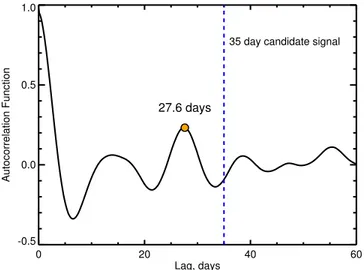
6. THE NON-TRANSITING PLANET KEPLER-20G In this section we argue that the planetary interpretation of the 35-day signal is more likely than a stellar activity interpretation. We measured the rotation period of Kepler-20 from the Kepler PDC-SAP light curves using an autocorrela-tion funcautocorrela-tion(ACF) analysis (e.g., McQuillan et al.2013). We
calculated the ACF for the full data set (quarters 1–17) and found a strong peak at a period of 27.6 days(see Figure7). The
signal near 27.6 days is persistent—we divided the data set in two, repeated the autocorrelation analysis on each half of the light curve, and found a peak at 27.0 days in thefirst half and a peak at 27.7 days in the second half. We interpret this 27.6 day signal as being caused by active regions on the stellar surface, and measure the rotation period of Kepler-20 to be
27.6±0.5 days. Furthermore, a periodogram of the FWHM measurements of the CCF function shows significant power at 27 days, indicating a stellar rotational period similar to that found from the photometry.
We believe it is unlikely that the period of the additional RV signal at 35 days is consistent with the stellar rotation period. The HIRES RV data were taken concurrently with Kepler observations(during the first half of the full Kepler data set). During this time, active regions on the stellar surface gave rise to a signal with a period of 27.0 days in theflux time series, while the additional RV signal (which was detected in the HIRES data alone) has a period of 35 days. These periods differ by 20%, and the ACF shows only a weak(negative) correlation betweenflux measurements taken 35 days apart.
However, in order to provide further evidence for the planetary nature of the signal, we perform further tests to show that it is not related to stellar activity. To do so, we removed the signatures of Kepler-20b, c, and d from the RVs, using our best fit, leaving only the 35-day signal. We then split the RV measurements into two equal chunks and estimated the generalized Lomb–Scargle (GLS) periodogram (Zechmeister & Kürster2009) for each of these chunks. Note that the power
in a GLS periodogram depends on the sampling and the total time span of the data. Therefore, to be able to compare the signals found in the two chunks, we needed to keep the same sampling and time span. For each chunk, we therefore kept the RV measurements outside of the chunk, butfixed their values to zero, with error bars of 100m s-1. A similar analysis was
performed forα Cen Bb (Dumusque et al.2012) and Kepler-10
(Dumusque et al.2014). In Figure4, we show the periodogram for each chunk of data(blue and red) and the GLS periodogram for the entire data set(gray). The signal at 35 days is shown in thefirst and second halves of the data, which is expected for a signal induced by a planet or by stellar activity if 35 days is the stellar rotation period. However, when looking at the phase of the signal, illustrated in Figure4by small arrows above the 35-day peak, it is clear that the signal has the same phase in each chunk. Furthermore, this phase is consistent with the phase derived when analyzing the entire data set. The signal thus retains the same phase from season to season, which is a strong argument in favor of the planetary origin of the signal. A signal due to stellar activity would change its phase because of the evolution of active region configuration on the stellar surface. To further assess the strength of the detection of the non-transiting planet, we calculated the S/N of the semi-amplitude of the signal for subsamples of the data. Wefirst performed the Bayesian General Lomb–Scargle periodogram (BGLS; Mortier et al. 2015) on the full data set. The strongest period in the
BGLS, which assumes a circular orbit, is 34.27 days. We then created subsamples of the data, starting with the first 30 data points and always adding one more data point. For each subsample, and fixing the period to 34.27 days, we found the best jitter term by calculating the maximum log likelihood of the model for a set of jitter values (spaced with 0.1m s-1).
Using this jitter term, we derived optimal scaling estimates for the semi-amplitude K and its variance sK
2
, ultimately giving the S/N of the signal over time: K/σK. From Figure8, it can be seen that the S/N roughly scales as a square root, as expected for a coherent signal in the data.
In summary, the tests described in this section strongly indicate that the signal at∼35 days is of planetary nature and Figure 4. GLS periodogram of the RV residuals (O–C) after removing our best
fit for Kepler-20b, c, and d. The black shaded periodogram corresponds to the analysis of the entire data set, while the red and blue periodograms correspond to thefirst and second halves of the data, respectively. The small arrows above the 35 day peak show the phase of the signal, which can rotate by 360° depending on the phase. The phases of the first and second halves of the data are compatible and also are compatible with the phase found for the entire data set. Therefore, the 35-day signal retains its phase as a function of time, which is expected for a planet. The top and bottom horizontal lines correspond to a FAP level of 1% and 10%, respectively
we therefore conclude that a non-transiting planet is present in the system with a period of34.940-+0.0350.038days.
7. STABILITY ANALYSIS
To investigate the stability of the Kepler-20 system, we carried out pure N-body simulations using mercury6 (Cham-bers 1999). We also carried out some tests using a 4th order
Hermite integrator (Makino & Aarseth 1992), but the results
from this were consistent with those from mercury6, so here we report only the results from the mercury6 simulations. We considered all six bodies, Kepler-20b, c, d, e, f, and g, orbiting a central star with mass M=0.9480.051M. The masses
of Kepler-20b, c, d, and g are taken from Table 4, while Kepler-20e is assumed to have a mass of Mp=0.65MÅ and
Kepler-20f is assumed to have a mass of Mp=1.0MÅ.
The initial semimajor axes are the same as in Table 4, and the system is assumed to be coplanar. The separation between adjacent planets, normalized to the mutual Hill radius, lies between 13 and 20, suggesting that the system lies outside the empirical stability limit of ∼10 (Chambers et al. 1996; Yoshinaga et al. 1999), and should therefore be long-term
stable if the eccentricities are sufficiently small. In our first test, we set the initial eccentricity for Kepler-20b to eb= 0.03 and set all the other eccentricities to e=0. With these initial conditions, the system is indeed stable for t>107 years (>5×10⁸orbits of Kepler-20d).
For Kepler-20c, the system is stable for eccentricities of ec0.17, and for Kepler-20g the system is stable for eccentricities of eg0.16, while for Kepler-20d the system is stable for eccentricities of ed0.28. Essentially, Kepler-20c and Kepler-20g appear to be constrained to have eccentricities well below e= 0.2, while Kepler-20d may have an eccentricity as high as e∼0.3.
We also considered scenarios where we varied the eccentricities of more than one of the planets. We again ran the simulations for 107years(5×10⁸orbits of Kepler-20d). If Kepler-20c has an eccentricity of ec= 0.1, then the system is only stable if Kepler-20g has an eccentricity of eg0.11. If Kepler-20g has an eccentricity of eg= 0.1 then the system is only stable if Kepler-20c has an eccentricity of ec0.11. If both Kepler-20c and Kepler-20g have eccentricities of
=
ec g, 0.1, then the system is stable if Kepler-20d has an eccentricity of ed0.22. As expected, if the eccentricities are non-zero, then the range of eccentricities for which the system is stable is reduced.
We should acknowledge that we have not run these simulations for longer than 107years. Hence, the system could still be unstable for the eccentricity values we present here, and consequently these should be regarded as upper limits. However, they do indicate that the eccentricities of Kepler-20c and g are likely to be constrained to be less than e∼0.2, while the eccentricity of Kepler-20d could be higher, but only if the others have relatively low eccentricities(e∼0.1 or less). Overall, the stability analysis appears to suggest that Kepler-20 is consistent with being a dynamically cold system in which the eccentricities and inclinations are small (Dawson et al. 2016), and it is a system that probably formed in the
transition phase when the disk had a high solid surface density, but a low to moderate gas surface density (Lee & Chiang2016).
8. SUMMARY AND DISCUSSION
We have revisited the mass determination of the planets in the Kepler-20 system. With a significantly increased number of RV measurements, an updated photometric analysis of the Kepler light curve, and an asteroseismic analysis of the parameters of the host stars, we present mass measurements of the three larger planets in the Kepler-20 system, as well as Figure 5. Mass–radius diagram for planets smaller than 3.2R with mass determinations better than 30% precision. The gray region to the lower right indicates theÅ
region where planets would have an iron content exceeding the maximum value predicted from models of collisional stripping(Marcus et al.2010). The solid curves are theoretical models for planet with a composition consisting of 100% water(blue), 25% silicate and 75% water (turquoise), 50% silicate and 50% water (magenta), 100% silicate(green), 70% silicate and 30% iron, consistent with an Earth-like composition (light blue), 50% silicate and 50% iron (brown), and 100% iron (red) (Zeng & Sasselov2013). The blue points indicate planets with masses measured using the HARPS-N spectrograph, purple points are from other sources, and the orange points are the Kepler-20 system with masses determined in this paper.
the detection of a non-transiting planet. With the refined analyses, we are able to reduce the uncertainty of the mass measurement of Kepler-20b to less than 15%. Kepler-20b has a mass of MP b, =9.70+-1.441.41MÅ(14.7%) and a radius of
Figure 6. Best–fit model (black solid curve) to the HARPS-N (blue points) and HIRES (green points) radial velocities when considering a model composed of the three largest transiting planets and the non-transiting planet in the Kepler-20 system. Each top panel show the phase-folder RVs after removing the orbital motion of the remaining planets. The red points show the weighted mean of the RVs binned to equal interval in phase. Each bottom panel shows the RV residuals after removing the full orbitalfit. The four plots show the orbital fit for Kepler-20b (top left), Kepler-20c (top right), Kepler-20g (bottom left), and Kepler-20d (bottom right).
Figure 7. Autocorrelation function of the Kepler-20 light curve. There is a peak in the autocorrelation function at 27.6 days, which we interpret to be the stellar rotation period. This is significantly different from the 35-day period of the RV variations, which we interpret to be a new non-transiting planet(shown as a blue dashed line).
Figure 8. S/N of the semi-amplitude for a signal with a period P=34.27 days (assuming a circular orbit) vs. number of data points. The solid line represents a square root function withy=0.61 x -0.96(best fit to the data).
= -+ Å
RP b, 1.868 0.0340.066R yielding a bulk density of r =b
-+
-8.2 1.3g cm
1.5 3. The precision allows us to conclude that
Kepler-20b has a composition consistent with a rocky terrestrial composition despite it large radius (∼1.9RÅ).
We also report the masses of 20c and Kepler-20d (Mp c, =12.75-+2.24MÅ 17.3%
2.17
( ), Mp d, =10.07-+3.70 3.97 Å
M (38.1%)) yielding densities indicating the presence of volatiles and/or a H/He atmosphere.
Furthermore, we report the detection of a non-transiting planet in the system (Kepler-20g) that has a minimum mass similar to that of Neptune (Mp g, =19.96-+3.613.08MÅ(16.7%)).
The orbital configuration of the Kepler-20 system has a rather large gap between 20f and 20d in which Kepler-20g is situated with an orbital period of∼35 days. In Section6
we find strong evidence for the signal at ∼35 days to be of planetary nature and not to be the result of stellar activity caused by spot modulation at the stellar rotational period.
Kepler-20b is thus the first definite example of a rocky exoplanet with a mass above 5MÅ and a radius larger than
1.6RÅ. This is seemingly at odds with the prediction that most
1.6RÅ planets are not rocky and larger planets are even more likely to exhibit lower bulk densities (Weiss & Marcy 2014; Rogers 2015). However, it is worth noting that all seven
planets in Figure 5 that have densities consistent with a rocky composition (Kepler-10b, Kepler-20b, Kepler-36b, Kepler-78b, Kepler-93b, HD 219134b, and CoRoT-7b) are highly irradiated, with a bolometric flux larger than
>
-Fv 2·10 J s5 1m2 (>146 times the flux received by the Earth). It is thus possible, and perhaps even likely, that we are measuring the masses of small planets in a particular part of parameter space that are hot and highly irradiated and could have lost their primordial gaseous envelope(if such envelopes were present) due to photoevaporation. If this is the case, we are thus measuring the masses of the bare cores of these planets.
Indeed, given the close-in orbit of Kepler-20b, and the likely low masses of Kepler-20e and f, we conclude that all three of these now likely rocky planets could have formed with significant gaseous envelopes that were subsequently lost to atmospheric photoevaporation(e.g., Lopez et al.2012) or other
processes such as impact erosion (e.g., Inamdar & Schlicht-ing 2015). Using the coupled thermal and photoevaporative
planetary evolution model of Lopez et al. (2012), we find that
the all the planets in the Kepler-20 system are consistent with a scenario in which each of the planets accreted a significant H/He envelope, composing 2%–5% of its total mass, but planets b, e, and f lost their envelopes, due to subsequent evolution. This is similar to the results found for a handful of other systems such as Kepler-36(e.g., Lopez & Fortney2013),
however, this type of evolutionary analysis is only possible for transiting systems with precise mass measurements.
It is important to significantly increase the number of precise mass measurements of transiting planets in order to populate the mass–radius diagram with planets of different sizes and masses at various orbital distances, including longer periods, that orbit a diverse sample of stellar types in order to fully appreciate the nature of the small exoplanets and their compositions.
The HARPS-N project was funded by the Prodex Program of the Swiss Space Office (SSO), the Harvard-University Origin of Life Initiative (HUOLI), the Scottish Universities Physics
Alliance (SUPA), the University of Geneva, the Smithsonian Astrophysical Observatory (SAO), and the Italian National Astrophysical Institute (INAF), University of St. Andrews, Queen’s University Belfast, and University of Edinburgh. The research leading to these results has received funding from the European Union Seventh Framework Programme (FP7/2007-2013) under Grant Agreement No. 313014 (ETAEARTH).
This work was performed in part under contract with the California Institute of Technology/Jet Propulsion Laboratory, which is funded by NASA through the Sagan Fellowship Program executed by the NASA Exoplanet Science Institute.
A.V. is supported by the NSF Graduate Research Fellow-ship, Grant No. DGE 1144152.
This publication was made possible by a grant from the John Templeton Foundation. The opinions expressed in this publication are those of the authors and do not necessarily reflect the views of the John Templeton Foundation. This material is based upon work supported by NASA under grant No. NNX15AC90G issued through the Exoplanets Research Program.
Funding for the Stellar Astrophysics Centre is provided by The Danish National Research Foundation (grant agreement no.: DNRF106). The research is supported by the ASTERISK project (ASTERoseismic Investigations with SONG and Kepler) funded by the European Research Council (Grant agreement no.: 267864). M.S.L. is supported by The Danish Council for Independent Research’s Sapere Aude program (grant agreement no.: DFF—5051-00130).
P.F. acknowledges support by Fundação para a Ciência e a Tecnologia (FCT) through Investigador FCT contract of reference IF/01037/2013 and POPH/FSE (EC) by FEDER funding through the program “Programa Operacional de Factores de Competitividade—COMPETE,” and further sup-port in the form of an exploratory project of reference IF/ 01037/2013CP1191/CT0001.
The research leading to these results also received funding from the European Union Seventh Framework Programme (FP7/2007-2013) under grant agreement number 313014 (ETAEARTH).
X.D. is grateful to the Society in Science–Branco Weiss Fellowship for itsfinancial support.
Software: SPC (Buchhave et al. 2012, 2014),
ECCSAM-PLES (Kipping 2014a), emcee (Fortney et al. 2013),
BAT-MAN(Kreidberg2015).
REFERENCES
Aerts, C., Christensen-Dalsgaard, J., & Kurtz, D. W. 2010, Asteroseismology (Berlin: Springer)
Auvergne, M., Bodin, P., Boisnard, L., et al. 2009,A&A,506, 411 Ballard, S., Chaplin, W. J., Charbonneau, D., et al. 2014,ApJ,790, 12 Baranne, A., Queloz, D., Mayor, M., et al. 1996, A&AS,119, 373 Batalha, N. M., Rowe, J. F., Bryson, S. T., et al. 2013,ApJS,204, 24 Bonomo, A. S., Sozzetti, A., Lovis, C., et al. 2014,A&A,572, A2 Borucki, W. J., Koch, D. G., Basri, G., et al. 2011,ApJ,736, 19
Buchhave, L. A., Bizzarro, M., Latham, D. W., et al. 2014,Natur,509, 593 Buchhave, L. A., Latham, D. W., Johansen, A., et al. 2012,Natur,486, 375 Burke, C. J., Christiansen, J. L., Mullally, F., et al. 2015,ApJ,809, 8 Chambers, J. E. 1999,MNRAS,304, 793
Chambers, J. E., Wetherill, G. W., & Boss, A. P. 1996,Icar,119, 261 Chaplin, W. J., & Miglio, A. 2013,ARA&A,51, 353
Cosentino, R., Lovis, C., Pepe, F., et al. 2012,Proc. SPIE,8446, 84461V Dawson, R. I., Lee, E. J., & Chiang, E. 2016,ApJ,822, 54
Dressing, C. D., & Charbonneau, D. 2013,ApJ,767, 95 Dressing, C. D., & Charbonneau, D. 2015,ApJ,807, 45
Dumusque, X., Bonomo, A. S., Haywood, R. D., et al. 2014,ApJ,789, 154 Dumusque, X., Pepe, F., Lovis, C., et al. 2012,Natur,491, 207
Ford, E. B. 2006,ApJ,642, 505
Fortney, J. J., Mordasini, C., Nettelmann, N., et al. 2013,ApJ,775, 80 Fressin, F., Torres, G., Rowe, J. F., et al. 2012,Natur,482, 195
Gautier, T. N., III, Charbonneau, D., Rowe, J. F., et al. 2012,ApJ,749, 15 Gettel, S., Charbonneau, D., Dressing, C. D., et al. 2016,ApJ,816, 95 Gilliland, R. L., McCullough, P. R., Nelan, E. P., et al. 2011,ApJ,726, 2 Haywood, R. D., Collier Cameron, A., Unruh, Y. C., et al. 2016,MNRAS,
457, 3637
Howard, A. W., Marcy, G. W., Bryson, S. T., et al. 2012,ApJS,201, 15 Inamdar, N. K., & Schlichting, H. E. 2015,MNRAS,448, 1751 Kipping, D. M. 2013,MNRAS,434, L51
Kipping, D. M. 2014a,MNRAS,444, 2263 Kipping, D. M. 2014b,MNRAS,440, 2164 Kjeldsen, H., & Bedding, T. R. 1995, A&A,293, 87 Kreidberg, L. 2015,PASP,127, 1161
Lasker, B. M., Lattanzi, M. G., McLean, B. J., et al. 2008,AJ,136, 735 Lee, E. J., & Chiang, E. 2016,ApJ,817, 90
Lopez, E. D., & Fortney, J. J. 2013,ApJ,776, 2
Lopez, E. D., Fortney, J. J., & Miller, N. 2012,ApJ,761, 59
López-Morales, M., Triaud, A. H. M. J., Rodler, F., et al. 2014, ApJL, 792, L31
Lundkvist, M., Kjeldsen, H., & Silva Aguirre, V. 2014,A&A,566, A82
Makino, J., & Aarseth, S. J. 1992, PASJ,44, 141 Mandel, K., & Agol, E. 2002,ApJL,580, L171
Marcus, R. A., Sasselov, D., Hernquist, L., & Stewart, S. T. 2010,ApJL, 712, L73
McQuillan, A., Mazeh, T., & Aigrain, S. 2013,ApJL,775, L11
Mortier, A., Faria, J. P., Correia, C. M., Santerne, A., & Santos, N. C. 2015,
A&A,573, A101
Pepe, F., Cameron, A. C., Latham, D. W., et al. 2013,Natur,503, 377 Pepe, F., Mayor, M., Galland, F., et al. 2002,A&A,388, 632
Petigura, E. A., Howard, A. W., & Marcy, G. W. 2013,PNAS,110, 19273 Rogers, L. A. 2015,ApJ,801, 41
Seager, S., & Mallén-Ornelas, G. 2003,ApJ,585, 1038
Sozzetti, A., Torres, G., Charbonneau, D., et al. 2007,ApJ,664, 1190 Tassoul, M. 1980,ApJS,43, 469
Torres, G., Winn, J. N., & Holman, M. J. 2008,ApJ,677, 1324 Ulrich, R. K. 1986,ApJL,306, L37
Valenti, J. A., & Fischer, D. A. 2005,ApJS,159, 141 Valenti, J. A., & Piskunov, N. 1996, A&AS,118, 595
Vogt, S. S., Allen, S. L., Bigelow, B. C., et al. 1994, Proc. SPIE, 2198, 362
Weiss, L. M., & Marcy, G. W. 2014,ApJL,783, L6 Yoshinaga, K., Kokubo, E., & Makino, J. 1999,Icar,139, 328 Zechmeister, M., & Kürster, M. 2009,A&A,496, 577 Zeng, L., & Sasselov, D. 2013,PASP,125, 227