Towards Aggregate Processes in a Field Calculus-Based Platform

(1)

ALMA MATER STUDIORUM – UNIVERSIT `

A DI BOLOGNA

CAMPUS DI CESENA

Scuola di Ingegneria e Architettura

Corso di Laurea Magistrale in Ingegneria e Scienze Informatiche

TOWARDS AGGREGATE PROCESSES IN A

FIELD CALCULUS-BASED PLATFORM

Relazione finale in

INGEGNERIA DEI SISTEMI SOFTWARE ADATTIVI

COMPLESSI

Relatore

Prof. MIRKO VIROLI

Co-relatori

Dott. ROBERTO CASADEI

Presentata da

DAVIDE FOSCHI

Terza Sessione di Laurea

Anno Accademico 2016 – 2017

(2)

(3)

List of Figures

1.1 Syntax of HOFC . . . 3

1.2 Aggregate Programming Stack . . . 6

2.1 Entities injecting and retrieving tuples (figure taken from [6]) . . 11

2.2 Examples of Replicated gossip instances (figure adapted from [7]) 12 2.3 Example of processes uncorrect alignment . . . 13

3.1 Architecture of the core library with alignment primitive . . . . 16

3.2 Aggregate process information and definition . . . 19

3.3 ProcessesLib architecture . . . 24

3.4 Spatial tuples library architecture . . . 26

3.5 Example of gossip replications (figure taken from [7]) . . . 30

4.1 Comparison between classic gradient and time-replicated gradi-ent in a stable condition . . . 47

4.2 Comparison between classic gradient and time-replicated gradi-ent after network changes . . . 48

(6)

(7)

Introduction

Nowadays, distributed systems are everywhere. They can be populated by smartphones, drones, sensors, vehicles, or any kind of device able to execute operations and interact with other devices. Heterogeneity is a key feature of complex distributed systems and represents a challenge for designers to handle communication between devices of different nature. Many coordination approaches are based on a individual-device view of the system and are not ideal, especially when systems grow in complexity, as they may suffer from design problems. Hence, a single-device view of the system forces designers to manage all the coordination issues, like resilience, fault-tolerance, etc. Finally, it is hard to maintain a full view of the system, so it is difficult to define a good global behaviour of the system.

Aggregate computing represents a prominent paradigm that aims to shift the view of system design from a local one to an aggregate viewpoint, in such a way that the whole system is programmed as a single entity, while interaction is made implicit. The work in [1], [2], [3] and [4] offer interesting developments related to aggregate computing by abstracting from the local view. Aggregate computing simply changes the way to observe ad define the behaviour of a distributed system. Therefore, the specifications of this global behaviour are locally mapped on each entity forming the system.

To enhance flexibility, aggregate computing requires mechanisms to smoothly change/adapt the behaviour of portions of the system over time. To do so, en-tities of the system should generate new tasks to be performed in a pro-active way, each of them defined as the composition of aggregate actions. Subse-quently, these tasks must be spread between entities in the network, forming different groups of entities.

(8)

The thesis discusses a concept for aggregate computing called Aggregate process, a computation generated in some node of the network and with some kind of spatial extension. This notion recalls and is inspired by a recent study related to aggregate programming where it is presented a way to fill the gap with multi-agent systems. Most specifically, the work in [5] introduces the notion of Aggregate Plan, which allows to define cooperative behaviour of dynamic teams of agents, resulting in a set of actions that each agent performs in order to achieve the goal that the plan is meant to reach.

Aggregate processes aims to expand current aggregate computing capabil-ity and expressiveness by proposing new constructs able to encapsulate the notion on aggregate process. User-friendly APIs will allow systems designers to specify more complex and dynamic behaviour with ease. Based on these ideas, in this thesis we propose an implementation of aggregate processes by exploiting a recently proposed platform based on field calculus and the Scala programming language, called scafi [3, 4].

To validate the need and the potential of aggregate processes, the thesis will present the implementation of some recent coordination models for distributed systems by exploiting this new concept. The models that have been chosen are the following:

• Spatial tuples [6], a tuple space based model featuring tuples with phys-ical position;

• Replicated gossip [7], an enhanced version of classic gossip protocols where time-dependent replications are used.

To summarize, the main goal of this thesis is to present an implementation of aggregate processes into scafi. The reminder of this document is organized as follow: Chapter 1 addresses the foundation of aggregate computing and the platform used in this project, Chapter 2 illustrate what has to be done and the main problem, Chapter 3 describes the proposed solution, Chapter 4 illustrates the technologies used for testing and its organization, and finally Chapter 5 offers an overview of the results achieved and introduces future works related to aggregate processes.

(9)

Chapter 1 Background

This chapter describes a set of studies that have been done in order to develop the notion of Aggregate processes into scafi.

Outline:

1. Aggregate Computing 2. Scafi

1.1 Aggregate Computing

This section introduces Aggregate computing as a promising approach for building large-scale, decentralised, adaptative, spatial systems. Hence, the following presents both the foundation of aggregate computing, Field calculus, and an overview of the studies related to aggregate computing.

1.1.1 Computational Fields and Field Calculus

Computational fields are introduced in a distributed environment where an aggregate of devices executes some kind of operations. They represent a way to map each device with a structured value. Many models, languages, and infrastructures have been create based on this concept. Fields tend to stabilize them-self after changes to the physical distribution of the devices and are robust to unexpected interaction that may disturb the computation.

(10)

2 CHAPTER 1. BACKGROUND They are thus suitable for the implementation of self-organizing coordination patterns [8].

Devices behaviours are defined by operations over fields. Such operations resemble functions that evolve, combine and restrict fields. Operations compo-sition allows to express the global behaviour of a distributed adaptive system, which means the overall computation occurs on the computational fields in the network. To describe the actual computation on a local-level, devices must execute a set of actions which comprehend local values manipulation and neighbourhood interactions.

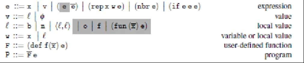
Fields Calculus is a way to define how to manipulate fields. The basic constructs are described below.

• Literals (l): Basic expression which represents a local value such as a number, a boolean, etc.

• Variables (v): Another basic expression used as a parameter of a function or to store a value.

• Built-in operators (o e1 ... en): Built-in function are standard mathe-matical functions and context-dependent operators. (o e1 ... en) rep-resents the point-wise evaluation of the operator over the input fields, which are mapped to a local value by each device.

• Function call (f e1 ... en): Allows to evaluate user-defined function on

a set of parameters. (def f(¯x) eB ) represents the definition of function f

where ¯x are the parameters and eB is the body of the function itself.

• Time evolution (rep x w e): This operator represents the concept of state, hence, the changes of a field over time. w is the initial value of the field, while e defines the expression that manipulate the field in respect of the last value of the field x.

• Interaction (nbr e): The nbr construct specifies how devices interact between each other and how information is spread between them. nbr maps each device to the neighbours evaluation of the field e. It is often used in combination with other hood-like operators, such as min-hood, to determine how to manipulate information taken from the neighbourhood.

(11)

CHAPTER 1. BACKGROUND 3

Figura 1.1: Syntax of HOFC

• Domain restriction (if e0 e1 e2 ): This mechanism defines a way the split the space of computation based on the conditional expression e0, which is evaluated everywhere. e1 is evaluated where e0 is true, while e2 is evaluated where e0 is false.

Higher-Order Calculus of Computational Fields Along with these mech-anisms, further studies, presented in [9], extend the capabilities of field calculus with First-order functions, so that code can be handled in a more dynamic way. The main differences can be seen above. Basically, the extension allows local values to be expressed as built-in and user-defined functions. Therefore, the calculus language gains the following advantages:

• functions can be defined on-the-fly as anonymous functions; • functions can be arguments of other functions;

• functions can shared in the neighbourhood with nbr construct; • functions evaluation may change over time via rep construct.

1.1.2 Aggregate Computing

In regards of spatial distributed system, most of the available paradigms focus on the definition of single devices computational behaviour and interac-tion. This narrows the view of a system as a whole because there are many technical aspects that must be addressed, for instance, implement a robust and efficient communication layer between single devices, able to withstand failures and topology changes in the network. A programmer needs to handle these problems simultaneously in order to define a good global behaviour of a distributed system.

(12)

4 CHAPTER 1. BACKGROUND To ease developers work, many studies brought to different approaches moving towards aggregate computing. Generally, they handle single or mul-tiple problems via abstraction. Non-functional features are supported in an implicit way. One of the most prominent is space-time computing, which de-fines devices in terms of physical position in space and interaction between each other and the space itself.

Aggregate computing extends the work on space-time computing. The main goal is to change the point of view from a local, single device view to a global one in order to focus on the global behaviour of the whole system. Devices forming a system are seen as a single abstract machine, so that it can be programmed as an individual.

Abstraction is the way to address the problems associated with distributed system. Aggregate programming offers implicit mechanism to handle these problems separately:

• device-to-device communication is made completely transparent to the programmer;

• basic construct allow to execute aggregate-level operations;

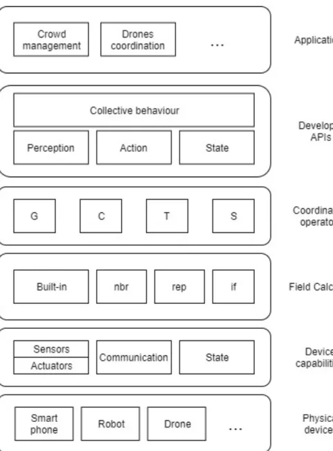
• system behaviour is define as a composition of aggregate-level operations. The work in [1] and [3] propose a set of building blocks for self-organizing applications, which identify coordination operators that can be used to define coordination patterns. These operators are the following:

• G(source, init, metric, accumulate): Also called gradient, this operator exploits the notion of distance to spread an information across the net. Two computations are executed simultaneously: on one hand it computes a field of distance to determine the current distance to the source. On the other hand, it computes a field by accumulating values along the gradient distance field away from the source;

• C(potential, accumulate, local, null): It is the complementary operator of G. Where G spreads information, C operator accumulates information. To do so, it uses a potential field to indicate the region the information must converge;

(13)

CHAPTER 1. BACKGROUND 5 • T(initial, floor, decay): This operator manages time interactions. Basi-cally, it works like a countdown, where initial is the timer starting values, decay function decreases the input value and floor is the timer threshold; • S(grain, metric): This operator is used to create partitions of devices. These blocks can be combined with each-other to define general-purpose APIs that can be used by the programmer to manage common coordination issues. The work in [1] and [2] propose several of these APIs.

Finally, the work in [2] proposes a stack for aggregate programming based on field calculus for Internet of Things applications:

• device capabilities are exploited to implement the basic field calculus constructs;

• these constructs are used to implement aggregate-level coordination Build-ing Blocks operators with resilience properties;

• on top of these, user-friendly APIs are developed to manage most com-mon scenarios.

(14)

6 CHAPTER 1. BACKGROUND

(15)

CHAPTER 1. BACKGROUND 7

1.2 Scafi

scafi is a platform for aggregate computing based on Scala and field calcu-lus. The entire process of analysis, design and development has been discussed in [4].

Aggregate Programming denotes a relatively new paradigm which change the way to design distributed system. It drifts the focus of programming from the single entities to the general behaviour of the system, hence it is particu-larly suitable for large-scale, adaptive, and pervasive systems.

Recent studies, like Proto or Protelis, offer aggregate programming ap-proaches based on Field calculus, allowing to define aggregate programs by compositions of computational fields, as seen in the previous sections.

However, these studies present ad-hoc solutions, which are suitable for a small group of application and are used as simulation tools. On the other hand, scafi proposes a more general-purpose framework that, ideally, could be used to develop real applications.

Scala programming language The language used to develop scafi was Scala for various reasons. First of all, Scala is supported by the JVM which in-tegrates smoothly both object-oriented and functional programming paradigms. Additionally, Scala offer the Akka library, an actor framework that comes handy when you have to develop distributed systems;

• it runs on JVM, which smoothly integrates both object-oriented and functional programming paradigms;

• it carries out many functional languages features, like type inference, lazy evaluation, currying, immutability and pattern matching [10]; • it is a scalable language, hence it keeps things simple with increasing

complexity.

Features As said before, scafi is a platform to program distributed system based on aggregate programming, field calculus and Scala language. At low level, scafi offers a domain-specific language (DSL) and a virtual machine (VM) with several characteristics:

(16)

8 CHAPTER 1. BACKGROUND • the language is fully embedded within Scala;

• the constructs of field calculus are supported;

• high-order field calculus is support too, even tho it has been necessary to introduce a new primitive to allow first-class function, called aggregate; • the language itself is pretty easy to use, concise and modular.

the work in [3] presents the implementation of the basic construct of field calculus and a few self-stabilising coordination operators.

The platform built on top of these DSL and VM provides APIs for the implementations of aggregate distributed systems:

• it offers spatial abstraction to support spatial computation;

• code mobility is support, hence the infrastructure is able to ship code between node in a transparent way;

• the platform is quite general-purpose, therefore it adapt to various sce-narios related to aggregate programming;

• pre-configurations are available to ease the initial setup of common sce-narios.

Finally, a simple simulator has been built over scafi to ease the development of distributed scenarios.

(17)

Chapter 2 Analysis

This chapter presents the analysis phase in the development of aggregate processes within scafi platform.

Outline:

• Notion of Aggregate processes • Systems examples

• The alignment problem • Work plan

2.1 Notion of Aggregate processes

Aggregate processes is an approach that aims to adopt the advantages brought by aggregate computing into the developing of distributed systems. The goal is to define coordination mechanism via aggregate computing, allow-ing to specify the spatial distributed systems behaviour as groups of entities that cooperate dynamically, hence each entity performs a set of actions based on physical location and neighbours interaction. An aggregate process defines the behaviour on a dynamic set of entities. A process is based on aggregate computing, so it supports functional composition, so complex behaviour can be achieved with ease. Processes are created by entities when a certain

(18)

10 CHAPTER 2. ANALYSIS tion is verified and spread across the network via neighbourhood interactions. An aggregate process can be described with the following features:

• a process can be generated in any entity of the network by verifying some kind of generation condition. In that case, the process is labeled as active;

• a process has a spatial extension, hence it spreads across the network until a certain distance threshold is met. Spatial extension can be cou-pled with other propagation conditions;

• multiple instances of the process may be active in the network at the same time. In that case, each instance must be independent from the others;

• when a node in the network owns multiple active processes instances, it has to execute all of them and spread evaluation information to the neighbours;

• a process defines a set of actions that each node has to perform;

• a process may be destroyed by the source node because of some kind of destruction condition.

2.2 Systems examples

The following presents examples of coordination models for distributed systems that intrinsically exploit a notion of process.

2.2.1 Statial Tuples

Spatial Tuples coordination model is an extension of the classic tuple space model where tuples have a location and eventually an extension in the physical space [6]. Tuples are physical entities that populate the environment together with devices. This model creates a sort of overlay which augment the information capability of the space, easing the definition of communication

(19)

CHAPTER 2. ANALYSIS 11

Figura 2.1: Entities injecting and retrieving tuples (figure taken from [6])

mechanisms. A tuple can be seen as a property which decorates a location of the space, thus devices can react to changes in the space, allowing to develop context-aware systems.

The basic primitives are the following:

• out(t @ r): Injects a tuple t in a location or region defined by r:

• rd(tt @ rt) and in(tt @ rt): Both operations allow to gather a random tuple which match the tuple template tt from a region that match the spatial template rt. While rd operation give back a tuple, if present, without eliminating it, the in operation consumes the tuple so that no one else can have access to that peace of information.

The figure 2.1 shows the behaviour of these operations. On the left, an out operation places a tuple into space with a certain spatial extension defined by a region. On the right, an out places a tuple in space while an entity located in that region attempts to gather the tuple with a rd operation.

In this context, the notion of aggregate process resides in the spatial man-agement of tuples: each tuple has a spatial extension granted by some kind of entities which handle in a transparent way the tuples location and propagation. With that said, each tuple can be interpreted as an aggregate process which is spread by nodes in the network. Each node can inject tuples by means of an out call. At the same time, a node may the source of a rd or a in function call in order to gather a tuple.

(20)

12 CHAPTER 2. ANALYSIS

Figura 2.2: Examples of Replicated gossip instances (figure adapted from [7])

2.2.2 Replicated Gossip

Replicated Gossip, proposed in [7], defines an extension of Gossip pro-tocols in which multiple instances of the gossip are kept alive simultaneously. It guarantees better responsiveness compared to classic gossip protocol. In replicated gossip, the presence of a notion of aggregate process is even more evident. Each single instance of gossip can be seen as process which is propa-gated in all the network and is computed by each node independently. Each replication, which is identified by a progressive number, has is own domain which is related to the value of the progressive number.

2.3 The alignment problem

In aggregate processes, the alignment problem emphasizes that processes, just like aggregate operations, must align between each other so that nodes can share information. In general, in an aggregate context, entities of the system must share information with other nodes in regards of certain aggregate operations in a way that these information do not interfere between each other. As described in the previous chapter, scafi is a platform based on field calculus for the development of distributed systems exploiting aggregate pro-gramming capabilities. Therefore, it is possible to define behaviour of the whole system at a higher level of abstraction, whereby behaviour is converted in a set of operations mapped on each entity. On top of that, scafi fully

(21)

sup-CHAPTER 2. ANALYSIS 13

Figura 2.3: Example of processes uncorrect alignment

ports HOFC, meaning that functions may be used as first-class entities. For these reasons, scafi is a suitable platform for the development of Aggregate processes.

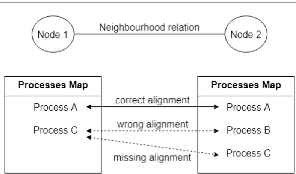
To better contextualize the alignment problem: scafi utilizes a value tree to describe each node computation. The order in which operation are inserted into the tree determine how these operations will align. Whenever a node executes an operation, a new entry is added to the value tree with a progressive index value. If different nodes have different operations on the same index value they can not interact because they are not aligned.

With the introduction of aggregate processes, it is legit to assume that a node may dynamically change his behaviour because processes are generated in the network. Because of that, each node may have a different map of processes to execute, hence each node can not align with his neighbours unless they have the same map of processes executed in the same order.

(22)

14 CHAPTER 2. ANALYSIS Consider the example proposed in figure 2.3: at a certain moment of time, each node possesses a map of processes as listed in the figure. Right now, it is not important how these nodes acquired their respective processes. With a or-der based alignment mechanism, Process A represents the best case scenario because both nodes execute the same process at the same level of the value true. Moving forward, nodes compute a different process, hence they do not align properly. On top of that, Process C do not align because it is execute at different levels on the value tree.

Drawing inspiration from the alignedMap construct proposed in [5], scafi proposes primitives to handle this alignment problem, with the end goal of supporting aggregate processes.

2.4 Work plan

System requirements have been defined in a incremental way, hence the development have been carried out by reaching progressively defined goals. The following presents a description of the work plan that brought to the implementation of aggregate processes into scafi :

• by assuming that an alignment mechanism with the features described previous was given, a set of basic constructs have been developed to formally define an aggregate process and handle generation and propa-gation of processes in a transparent way;

• finally, a library have been developed by exploiting the basic construct for aggregate processes to facilitate the use of this notion to define com-plex system behaviours. On top of that, more libraries have been added to support the coordination models introduction in the sections above, Spatial tuples and Replicated Gossip;

• at the same time, all libraries add been paired with functional testing to demonstrate robustness and reliability of these libraries over multiple scenarios.

(23)

Chapter 3 Design and Implementation

The development of this project has been heavily influenced by the technical aspects of scafi. Mainly, the general development approach is in line with a generic bottom-up approach, where you start from individual parts of the system. Because of that, the design phase has been intrinsically related to the implementation.

This chapter describes the development process of aggregate processes by presenting, in order, each part of the system.

Outline:

1. Alignment mechanism

2. Basic constructs for Aggregate processes 3. Processes Library

4. Coordination models design and implementation

(24)

16 CHAPTER 3. DESIGN AND IMPLEMENTATION

3.1 Alignment mechanism

Figura 3.1: Architecture of the core library with alignment primitive

Alignment mechanism is related to computation domain alignment, hence

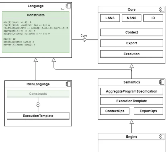
it is defined as a new basic construct of field calculus. The above figure,

originally presented in [4], highlights the main components of scafi core library. In this context, Language component defines the basic construct of the DSL proposed by scafi based on the primitives proposed by field calculus.

scafi was already extended with an align primitive inspired by previous works, with the following signature: align[K, V](key: K)(comp: K): V

It allows to specify a key on which the computation comp is aligned, hence the computation domain of comp is, in some way, related to the value of key.

(25)

CHAPTER 3. DESIGN AND IMPLEMENTATION 17

3.2 Basic constructs for Aggregate processes

3.2.1 Generation and propagation mechanisms

Each node of the network must be able to generate processes and to gather information related to other processes from the neighbourhood, hence each node contributes to the spatial propagation of all processes generated in the network.

Each round, a node evaluates generation and destruction conditions to determine if a new process has to be injected in the space or an old process has to be destroyed.

The propagation of processes is the critical part because interaction is pos-sible by exploiting a neighbourhood notion, hence each node is aware of the information evaluated by nodes situated within a certain distance. Because of that, a node can not perceive directly when and where the source node of a process has destroyed the process itself, unless the source of that process is located in his neighbourhood. The destruction signal of the process must travel everywhere exploiting peer-to-peer like communications: if the network is spatially large, there may be some latency.

On top of that, occasional failure of nodes can happen in real applications. Obsolete information related to processes may remain into nodes that failed to execute, or simply detach from the network. It must be impossible for nodes with outdated information to contaminate the network with these kind of information.

The following presents a set of information that define the state of a process at a given time. These information are elaborated by a node to understand the current situation and determine how to manage that process in terms of evaluation and propagation. Each node maintains a map of these information: each entry of the map represents a single process instance.

• ID: Identifier of the process;

• D: Distance to the source of the process; • L: Propagation limit of the process;

(26)

18 CHAPTER 3. DESIGN AND IMPLEMENTATION • C: Liveness of the process.

On top of these information, propagation mechanisms have been realized to ensure a safe propagation of processes. These mechanisms are summarized by a set of rules:

• when a node verifies certain conditions, it injects a new process with a unique identifier where distance D is zero and the liveness information C is some well defined value. Each round, the source update the value of C ;

• when the source wants to destroy a process, it sets the value of C to undefined ;

• given a certain node, for each active process the node analyzes all the neighbours and determines the closest which neighbour is the closest to the source of that particular process. After that, the node gathers the liveness information C of the process from that neighbour. This mechanism ensure that a process is always propagated outwards, so that nodes closer to the source, which are more sensible to source changes, are more relevant in the propagation process. A node located far away from the source can not disrupt the global propagation of a process with obsolete information;

• nodes gather new processes in the following way: given a certain node, for each process in each neighbour, the process is valid if the distance to the source stays within the limit L and the value of C is define. The result is a projection of all processes situated in the neighbourhood can have to be executed in that particular node;

• the value of C determines when a process has been destroyed or not. If C changes each round the process is still active. When C does not change for a certain amount of time, it means that the source (the only node that autonomously update C ) has destroyed the process. This liveness information prevents the propagation of processes from fake sources. All these information and mechanisms are exploited to define basic primi-tives, called Spawn and Fork that are presented in the sections below.

(27)

3.2.2 Formal definition of aggregate process

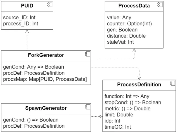
Figura 3.2: Aggregate process information and definition

PUID defines a unique identifier for a instance of a process. In fact, the identifier management requires a few considerations: the same process may be generated in multiple nodes of the network, hence the identifier must be the combination of different values. A identifier must depend on both the source of the node and the definition of the process itself. In this implementation, the process identifier is defined as a pair of positive integer where source ID is the identifier on the source node and process ID is the identifier associated to the process definition.

ProcessDefinition component formalizes all the features of a process: • function represents the computation associated to that process. It takes

(28)

20 CHAPTER 3. DESIGN AND IMPLEMENTATION • stopCond allows to the define the descruction condition of the process; • metric represents the distance function used to determine how nodes

evaluate the distance to the source of the process; • limit represents the spatial limitation of the process;

• idp represents the identifier associated to the process. As introduced before, the identifier management is a crucial aspect. In fact, idp must be unique across the network: each different process definition must have a different idp value;

• timeGC is the garbage collection timer threshold. As said before, pro-cess are locally destroyed by nodes when the value liveness information remains the same for a certain amount of time. timeGC allows to specify how much time a node has to wait before destroying the process.

ProcessData component defines all the information used by a node the manage a process state:

• value represents the evaluation of the function associated to the process in a node;

• counter is the implementation of the liveness information discussed be-fore. This value is increment by the source of the process at each round. When counter remains the same for a certain amount of time, the value is nullified. As said before, undefined counter means the source is noti-fying all other nodes that the process needs to be destroyed. If the value of counter remains undefined for a certain amount of time the process is locally removed;

• gen is an information used by the source of the process to keep track of the status of the process itself;

• distance represents the current distance to the source node of the process and is update whenever the topology of the network changes;

(29)

CHAPTER 3. DESIGN AND IMPLEMENTATION 21 • staleVal keeps track of the steadiness of counter. staleVal is incremented

whenever the counter remains the same, otherwise is reset to zero. SpawnGenerator and ForkGenerator exploit ProcessDefinition to de-fine different ways to generate aggregate processes. The key difference concerns the generation condition of the process itself. On one hand, SpawnGenerator defines the condition as a 0-ary function based on the local context of a node. On the other hand, ForkGenerator offers a more interesting way to specify the generation condition of a process. In particular, it allows to verify the generation condition on the domain of other processes.

3.2.3 Basic construct for process management: Spawn

Spawn is the most basic primitive able to handle processes generation and propagation as described in previous sections. In particular, generations is made by evaluating a condition over information which are not related to processes, e.g. verifying if a sensor has been trigger or not.

The whole body the Spawn is embedded into a rep call. The rep operates over a tuple of values representing, respectively, the current map of all the active process and the combination of generation and destruction condition. This combination simplifies the local process generation and destruction.

Inside rep, the computation is organized in four major blocks:

• first of all, foldhoodPlus gathers all the processes, both old and new, located in the neighbourhood following the rules defined in previous sec-tions. The result is a map of processes;

• after that, these processes are elaborated in order to update local active processes, while maintaining new processes;

• the map of processes is then filtered, hence all processes where the stal-eVal exceed the threshold timeGC and the counter is undefined are eliminated. At the same time, active prosesses are computed with the use of the align operator;

• finally, the process map is completed by adding, if needed, the process generated locally by a node.

(30)

22 CHAPTER 3. DESIGN AND IMPLEMENTATION Spawn has been conceived as a primitive able to handle the propagation of all processes defined by spwDef. This means that when a node makes a spawn function call with a certain process definition, spawn manages the local generation of the process and the propagation of all the instances of that process that are located in the network. Because of that, the return value of spawn is not a single process, but a map of processes.

def spawn(spwDef: SpawnGenerator): Map[PUID, ProcessData] = {

val local_idp = PUID(mid(), spwDef.procDef.idp)

def processComputation(idp: PUID): Option[Any] = align(idp){ key =>

Some(spwDef.procDef.function(key.source_ID)) }

rep[(Map[PUID, ProcessData], Boolean)]((Map[PUID, ProcessData](local_idp -> ProcessData()), false)) {

case (localPs, genCond) =>

val isGen: Boolean = mux(spwDef.procDef.stopCond())(false)(genCond || spwDef.genCond())

val localGen = localPs.apply(local_idp)

// gather all processes from the neighbourhood

(foldhoodPlus[Map[PUID, ProcessData]](localPs)((currentMap, newMap) => { currentMap ++ newMap.filter { case (newIdp, newData) =>

currentMap.get(newIdp) match {

case Some(oldData) => newData.distance <= oldData.distance

case None => newData.distance < spwDef.procDef.limit && newData.counter.isDefined }

}

})(nbr(localPs).map { case (idp, data) =>

idp -> ProcessData( value = None,

counter = data.counter,

distance = data.distance + spwDef.procDef.metric(),

staleVal = if (localPs.contains(idp)) localPs.apply(idp).staleVal else 0 )

})

// maintain new processes and update local active processes

.map { case (newIdp, newData) =>

localPs.get(newIdp) match {

case Some(oldData) =>

newIdp -> mux(oldData.staleVal < spwDef.procDef.timeGC)(ProcessData(

value = if (newData.counter.isDefined) processComputation(newIdp) else None, counter = newData.counter,

distance = newData.distance,

staleVal = if (newData.counter == oldData.counter) oldData.staleVal + 1 else 0 ))(ProcessData(

distance = newData.distance,

staleVal = if (oldData.counter.isDefined) 0 else spwDef.procDef.timeGC ))

case None =>

(31)

value = if (newData.counter.isDefined) processComputation(newIdp) else None ))

} }

// modify and destroy terminated processes

.filter { case (_, newData) => !(newData.staleVal >= spwDef.procDef.timeGC && newData.counter.isEmpty) }

// local generation management

+ (local_idp -> mux(isGen || (localGen.gen && localGen.staleVal < spwDef.procDef.timeGC)) {

ProcessData(

value = if (isGen) processComputation(local_idp) else None,

counter = if (isGen) Some(localGen.counter.map(_ + 1).getOrElse(0)) else None, gen = true,

distance = 0.0,

staleVal = if (isGen) 0 else localGen.staleVal + 1 ) } { ProcessData(staleVal = spwDef.procDef.timeGC) }), isGen) }._1 }

3.2.4 Managing complex processes generation: Fork

At a certain point of the development process, an interesting questions came into mind: may a process generate others processes? Hence, can the local evaluation of a process trigger some kind of condition which cause the generation of a different process with its own definition and rules?

These questions brought to the development of a new primitive called fork. The goal of this primitive is to allow the definition of processes which are gen-erated by evaluation some conditions over fields gengen-erated by other processes in the network.

Spawn allow to specify processes generation in a different way, but is able to handle the propagation just fine. Because of that, fork may exploit spawn by changing the generation management and evaluation.

The following presents the implementation of fork. The generation condi-tion is a 1-ary funccondi-tion evaluated over a map which contains the evaluacondi-tion of all processes.

(32)

def fork(fork_def: ForkGenerator): Map[PUID, Any] = { spawn(SpawnGenerator(

genCond = () => fork_def.procsMap.values.count(v => fork_def.genCond(v)) > 0, procDef = ProcessDef( function = fork_def.procDef.function, stopCond = fork_def.procDef.stopCond, metric = fork_def.procDef.metric, limit = fork_def.procDef.limit, idp = fork_def.procDef.idp, timeGC = fork_def.procDef.timeGC

))).collect { case (puid, ProcessData(Some(v),_,_,_,_)) => puid -> v } }

3.3 Processes Library

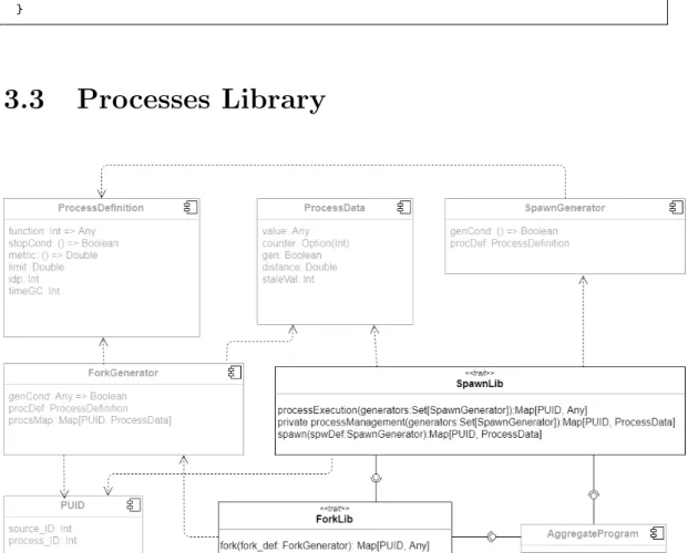
Figura 3.3: ProcessesLib architecture

ProcessesLib presents a wrap of spawn and fork primitives. Each sub-library is defined as an extension of AggregateProgram, so that basic con-structs are available.

(33)

pro-CHAPTER 3. DESIGN AND IMPLEMENTATION 25 cesses generation and propagation. In particular, processExecution allows to gather all processes computation by passing a list of processes definition as a parameter. Internally, each process definition is handled separately. At the same time all information used to manage generation, propagation and destruction of a process are completely transparent.

At the moment, ProcessesLib do not add to much capabilities to the already described spawn and fork primitives. However it is a good starting point for the development of a virtual machine with interesting features.

package lib

import it.unibo.scafi.incarnations.BasicSimulationIncarnation._

import scala.util.Try

case classProcessData(value: Option[Any] = None, counter: Option[Int] = None, gen: Boolean = false,

distance: Double = Double.PositiveInfinity, staleVal: Int = 0)

case classPUID(source_ID: Int, process_ID: Int)

case classProcessDef(function: Int => Any,

stopCond: () => Boolean = () => false, metric: () => Double,

limit: Double = Double.PositiveInfinity, idp: Int,

timeGC: Int = 100)

case classSpawnGenerator(genCond: () => Boolean, procDef: ProcessDef)

case classForkGenerator(genCond: Any => Boolean, procsMap: Map[PUID, Any], procDef: ProcessDef)

trait SpawnLib {

self: AggregateProgram =>

def processExecution(generators: Set[SpawnGenerator]): Map[PUID, Any] =

processManagement(generators).collect {

case (puid, ProcessData(Some(v),_,_,_,_)) => puid -> v }

private def processManagement(generators: Set[SpawnGenerator]): Map[PUID, ProcessData] = { (for (gen <- generators) yield { spawn(gen) }).fold(Map())((a,b) => a ++ b)

}

def spawn(spwDef: SpawnGenerator): Map[PUID, ProcessData] = ??? }

trait ForkLib {

self: AggregateProgram with SpawnLib =>

def fork(fork_def: ForkGenerator): Map[PUID, Any] = ??? }

(34)

3.4 Coordination models design and

implemen-tation

The following proposes libraries that have been developed to support the use of spatial tuples and replicated gossip as coordination models.

3.4.1 Spatial Tuples

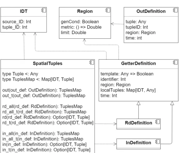
Figura 3.4: Spatial tuples library architecture

IDT component defines a unique identifier or each tuple. It resembles the identification mechanisms used to identify aggregate processes. In fact, tuple behavior have been implement by exploiting the notion of aggregate process.

Region component has multiple purposes: it is used to describe the spatial location of a tuple and to describe the physical extension of a getter primitives

(35)

CHAPTER 3. DESIGN AND IMPLEMENTATION 27 (both rd and in).

OutDefinition component defines the basic out primitive. When a tuple is injected in the network, it behaves just like an aggregate process. A map of tuples is returned because it is needed for other primitives to work properly.

GetterDefinition defines the getter primitive of Spatial tuples coordina-tion model and in inherited by RdDefinicoordina-tion and InDefinicoordina-tion. Because side-effect is an issue in this kind of development environment, the library can not keep track of tuples that have been injected in the space by using variables. Hence getter primitives take a parameter localTuples which represents a map of all tuples that are locally active.

SpatialTuples component implements most of the spatial tuples prim-itives and their respective timed version and bulk version, as shown in the following.

Before showing the actual library implementation, a short annotation is needed: the understanding process of how to handle tuples generation, local-ization and propagation was not trivial. Several attempts and quite some time were needed to get a clear vision of how tuples should behave in the scafi en-vironment. Because of that in primitives where not implemented. This does not mean that scafi and aggregate processes are not able to fully support the Spatial tuples model. In fact, the following shows the current implementation of all out and rd primitives, which exploit spawn primitive to handle tuples in terms of generation, spatial localization and spatial extension. On top of that, a more technical description is given to better understand the implementation of some critical aspects.

override def out(out_def: OutDef): TuplesMap = {

rep[(TuplesMap, Option[Any])](Map(), None){ case (_, tuple)=> val tuples: TuplesMap = spawnTuple(out_def.copy(

tuple = Try(tuple.get) getOrElse "empty",

region = out_def.region.copy(genCond = out_def.region.genCond))) (

tuples,

if(tuples.nonEmpty && tuple.isEmpty) Some(out_def.tuple) else tuple )

}._1 }

(36)

rep[(TuplesMap, Int, Option[Any])]((Map(), out_def.time, None)){ case (_, t, tuple) => val tuples = spawnTuple(

out_def = out_def.copy(

tuple = Try(tuple.get) getOrElse "empty",

region = out_def.region.copy(genCond = out_def.region.genCond)), stopCond = t - 1 <= 0)

( tuples,

mux(tuples.isEmpty)(out_def.time)(t - 1),

if(tuples.nonEmpty && tuple.isEmpty) Some(out_def.tuple) else if(tuples.nonEmpty) tuple else None

) }._1 }

private def spawnTuple(out_def: OutDef, stopCond: Boolean = false): TuplesMap = { align("out" + out_def.tupleID)(_ => spawn(

SpawnGenerator(

genCond = () => out_def.region.genCond,

procDef = ProcessDef(function = _ => out_def.tuple, stopCond = () => stopCond,

metric = out_def.region.metric, limit = out_def.region.limit, idp = out_def.tupleID)) )).filter( _._2.value.isDefined)

.map{ case (idp, data) => IDT(idp.source_ID, idp.process_ID) -> data.value.get } }

In spatial tuples, whenever a tuple is injected into the space, it remains there until a in operation consumes it. On top of that, the tuple should not be able to change value over time, even tho a notion a ”live tuple” exists but is not considered in this implementation. A rep is used to keep track of the tuple behaving like a state value: when the tuple is locally generated, the rep keeps the current value of the tuple. TuplesMap is a support map to memorize all tuples that are propagating through a certain node. The timed counter also keeps track of a timer. When the threshold is met, the tuple is destroyed.

override def rd_all(rd_def: RdDef): TuplesMap = { rep[TuplesMap](Map())(m => {

val read: TuplesMap = align[String, Map[PUID, ProcessData]]("read" + rd_def.rdID)(_ =>

spawn(SpawnGenerator(

genCond = () => rd_def.region.genCond, procDef = ProcessDef(

function = id => {

C[Double, TuplesMap](myG[Double](id, 0.0, _ + rd_def.region.metric(), rd_def.region.metric()),

(37)

_ ++ _, rd_def.localTuples.filter{case (_, tuple) => rd_def.template(tuple)}, Map())

},

metric = rd_def.region.metric, limit = rd_def.region.limit,

idp = rd_def.rdID)))).get(PUID(mid(), rd_def.rdID)) match {

case Some(d) => Try(d.value.get.asInstanceOf[TuplesMap]).getOrElse(Map())

case None => Map() } branch(rd_def.region.genCond){ m ++ read } { Map() } }) }

Among all rd primitive versions, rd all is the most generic of all. Others rd can be seen as a specialization of rd all. In fact, as the code shows, all rd have been implemented by reusing rd all primitive. The main role of the rep is to memorize the tuples that been read. A C function call is used to gather tuples that the given template. When there is a match, all tuples are memorized and will not change even if the original tuple is consumed by a in operation.

override def rd_all_t(rd_def: RdDef): TuplesMap = {

rep[(TuplesMap, Int)]((Map(), rd_def.time)){ case (tupleMap, t) => val tuples = rd_all(RdDef(

template = rd_def.template, rdID = rd_def.rdID, region = rd_def.region, localTuples = rd_def.localTuples) ) (branch(rd_def.region.genCond && t > 0){ tupleMap ++ tuples } { Map() }, mux(rd_def.region.genCond)(t - 1)(rd_def.time)) }._1 }

override def rd(rd_def: RdDef): Option[(IDT, Tuple)] = { rd_all(RdDef( template = rd_def.template, rdID = rd_def.rdID, region = rd_def.region, localTuples = rd_def.localTuples) ).collectFirst[(IDT, Tuple)]({

(38)

case t: (IDT, Tuple) => t })

}

override def rd_t(rd_def: RdDef): Option[(IDT, Tuple)] = { rd_all_t(RdDef( template = rd_def.template, rdID = rd_def.rdID, region = rd_def.region, time = rd_def.time, localTuples = rd_def.localTuples) ).collectFirst[(IDT, Tuple)]({

case t: (IDT, Tuple) => t })

}

rd all t adds an integer value used to manage time, just like out t. Both rd and rd t exploit rd all by collecting one of the tuples that have been found.

3.4.2 Replicated Gossip

The library recalls the implementation proposed in [7]. Replicated gossip has the following parameters:

• f : gossip protocol which is compute in every node of the network; • x: indicates the first value associated to new replications;

• k: indicates how many replications are kept alive;

• d: indicates an estimation of the diameter of the network graph.

(39)

CHAPTER 3. DESIGN AND IMPLEMENTATION 31 Every round, each node verifies if a new replication has to be created by consulting a timer. This timer is determined with a formula, which is the result of an analysis phase conducted and proposed in [7]. This analysis shows that each replication needs time to stabilize. Because of that, the value of older replication are the one that must be used until the newer replications have become stable. The result of the formula indicated a safe estimation of the time need by each replication to stabilize.

In aggregate computing, the next node to compute is chosen in a completely non-deterministic way. Because of that, each node may have different value of timers at the same time. A notion of sharedTimer is introduce to avoid complete desynchronization of replications between nodes. Given a node, if the timer condition is locally triggered or a neighbour has a newer replication, then it locally generates a new replications. Replications are identified by a progressive positive number, so it possible to determine which replication is the newest among the others. This number is exploited to guarantee a correct computation of all replications. In particular, the domain of each replication must not interfere with other domains. align construct handles this problem by using the progressive number as an alignment key.

The following presents the actual library implementation for replicated gossip. package lib import it.unibo.scafi.incarnations.BasicSimulationIncarnation._ import sims.SensorDefinitions import scala.util.Try trait ReplicatedGossip {

self: AggregateProgram with SensorDefinitions => def gossip[V](f: (V, V) => V, x: V): V = {

rep(x) { v =>

f(x, foldhoodPlus[V](v)((a, b) => f(a, b))(nbr(v))). }

}

def replicatedGossip[V](f: (V, V) => V, x: V, k: Int, d: Int): V = {

val p = 4 * d * deltaTime() / (k - 1)

timeReplication[V](() => gossip(f, x), x, p.toMillis.toInt, k).minBy(_._1)._2 }

(40)

def timeReplication[V](process: () => V, default: V, t: Int, k: Int): Map[Int, V] = { rep(Map[Int, V]())(replicate => {

val newRep = sharedTimer(replicate.keySet, t)

val procs = if (newRep > 0) { replicate + (newRep -> default) } else {

replicate }

val res = foldhood[Map[Int, V]](Map())((a, b) => { a ++ b

})(nbr(procs)).map { case (repID, _) => repID -> align(repID)(_ => process()) }

val maxRep = Try(res.keySet.max) getOrElse 0

res.filter { case (repID, _)=> (maxRep - repID) < k } })

}

def sharedTimer(replicate: Set[Int], t: Int): Int = {

var newReplicate = 0

rep((0, 0)) { case (topRep, time) =>

val maxID = math.max(topRep, Try(replicate.max) getOrElse 0)

if (maxID > topRep) { (maxID, t) } else if (time <= 0) { newReplicate = maxID + 1 (maxID + 1, t) } else { (topRep, time - 1) } } newReplicate } }

(41)

Chapter 4 Testing

In software engineering, testing represents an important activity. For this project, testing as been used not only to verify the correctness of all libraries and primitives, but also to speed up the development process. From the be-ginning, testing scenarios have been defined to better understand behaviour requirements of each construct.

All test cases have been realized by using ScalaTest1 _{testing tool. In}

order to properly replicate the necessary scenarios, few functions have been implemented to better simulate changes in network topology, neighbourhood relationships and nodes execution.

def detachNode(id: ID, net: Network with SimulatorOps): Unit = { net.setNeighbourhood(id, Set())

net.ids.foreach(i => {

net.setNeighbourhood(i,net.neighbourhood(i) - id) })

}

def connectNode(id: ID, nbrs: Set[ID], net: Network with SimulatorOps): Unit = { net.setNeighbourhood(id, nbrs)

nbrs.foreach(i => {

net.setNeighbourhood(i,net.neighbourhood(i) - id) })

}

def execProgramFor(ap: AggregateProgram, ntimes: Int = DefaultSteps) (net: Network with SimulatorOps)

(when: ID => Boolean, devs: Vector[ID] = net.ids.toVector, rnd: Random =

1_{http://www.scalatest.org/}

(42)

34 CHAPTER 4. TESTING

new Random(0)): Network ={

if(ntimes <= 0) net

else{

val nextToRun = until(when){ devs(rnd.nextInt(devs.size)) } net.exec(ap, ap.main, nextToRun)

execProgramFor(ap, ntimes-1)(net)(when, devs, rnd) }

}

• detachNode allow to detach a node from the network, hence the neigh-bours map of each node is update to reflect the detachment operation. • connectNode operates in the opposite way, so the node is reintegrated

into the network.

• execProgramFor allow to decide which nodes computed the aggregate program and which nodes do not. In combination with detachNode, a node can be completely ”turn off”, in the sense that it does not compute and does not interact with other nodes.

To avoid general disorder, code have been properly modified to better ex-emplify the goals of these tests. Scenarios are simulated by a simple network formed by few nodes arranged in a grid-like formation. For each node, its neighbors are the direct nodes located at the top, bottom, left and right with distance equal to one.

The following presents each library testing environment by describing in detail the scenarios that have been simulated. Basic scenarios are proposed for multiple libraries and they will be described on the first occurrence.

4.1 Processes libraries

The most important part of the whole testing phase has been creating a testing environment to verify the correctness of aggregate processes primitives, which are the fundamental parts of the whole project. The following describes how spawn and fork primitives have been tested.

(43)

CHAPTER 4. TESTING 35

4.1.1 Spawn primitive testing

In order to verified the correctness over different scenarios, a simple ag-gregate program have been defined. In particular, the program specify two different processes. Each process is generated and destroyed by sensing the

change in sense1 and sense2. The function bounded to each process is a

gradient-like operation that evaluated the distance from the source of the pro-cess itself. The function is the same for both propro-cesses. Propro-cessesLib APIs are used for better readability.

private[this] class Program extends SpawnLib with ForkLib

with AggregateProgram with StandardSensors with MyG {

override type MainResult = Any

override def main(): Any = {

def sense1 = sense[Boolean]("sense1")

val spawnDefs = Set( SpawnGenerator( genCond = () => sense1, procDef = ProcessDef( function = id => f"${myDistanceTo(id)}%.1f", stopCond = () => !sense1, metric = nbrRange, limit = 4.5, idp = 1)), SpawnGenerator( genCond = () => sense2, procDef = ProcessDef( function = id => f"${myDistanceTo(id)}%.1f", stopCond = () => !sense2, metric = nbrRange, limit = 2.0, idp = 2)) ) processExecution(spawnDefs) } }

Starting from simplest cases, a process must or must not exist depending on the evaluation of the generation condition.

Processes must "not exist if not activated" in new SimulationContextFixture {

// ACT

exec(program)(net)

// ASSERT

(44)

}

Processes must "exist when activated" in new SimulationContextFixture {

// ACT

exec(program, ntimes = 500)(net)

// ASSERT

assertForAllNodes[ProcsMap] { (_, m) => m.forall(_._2 == None) }(net)

// ARRANGE

net.chgSensorValue("sense1", Set(8), true)

// ACT

// ASSERT

val p81 = PUID(8, 1)

assertNetworkValues[ProcsMap]((0 to 8).zip(List(

Map(p81 -> "4,0"), Map(p81 -> "3,0"), Map(p81 -> "2,0"), Map(p81 -> "3,0"), Map(p81 -> "2,0"), Map(p81 -> "1,0"), Map(p81 -> "2,0"), Map(p81 -> "1,0"), Map(p81 -> "0,0") )).toMap)(net)

}

A process has a spatial extension which is limited by some kind of threshold. sense2 is associated to process with extension limit equals to two. Because of that further nodes from the source will not perceive the process.

Processes can "have a limited extension" in new SimulationContextFixture {

// ARRANGE

// ACT

// ASSERT

Map(p02 -> "0,0"), Map(p02 -> "1,0"), Map(p02 -> "2,0"), Map(p02 -> "1,0"), Map(p02 -> "2,0"), Map[PUID, String](), Map(p02 -> "2,0"), Map[PUID, String](),Map[PUID, String]() )).toMap)(net)

}

A process must be destroyed when the source verifies a certain condition. In this case, a process is generated and then destroyed by changing the value of sense1. The assertions show the expected value of nodes in the network.

Processes can "be extinguished when stopped being generated" in new SimulationContextFixture {

(45)

// ACT (process activation)

// ASSERT

// ACT (process deactivation and garbage collection)

net.chgSensorValue("sense1", Set(0), false) exec(program, ntimes = 2000)(net)

// ASSERT

assertForAllNodes[ProcsMap] { (_, m) => m.forall(_._2 == None) }(net) }

Processes propagation is fundamental and has to persist even went failures occur. In this scenario, a node failure is simulated to verify robustness and reliability of the spawn primitive:

• first of all, a process is generated by a node in the network;

• after that, a node (different from the source) is deactivated, so that it keeps track of the result of the its last round;

• meanwhile, the process is destroyed, hence the source node stop to gen-erate the process. Assert 2 shows that after a certain number of rounds, all nodes must not have the original process except the deactivated one; • finally, that node is reattached to the network and all nodes execute several rounds. In the end, the process must not exist in any of the nodes.

Node must "not interfere with others processes when it has obsolete process data" in new

SimulationContextFixture {

// ARRANGE

(46)

// ASSERT #1

// ARRANGE

net.chgSensorValue("sense1", Set(0), false) detachNode(1, net)

// ACT

execProgramFor(program, ntimes = 10000)(net)(id => id != 1)

// ASSERT #2

assertForAllNodes[ProcsMap] { (id, m) =>

id == 1 && m == Map(p01 -> "1,0") || m.forall(_._2 == None) }(net)

// ARRANGE

connectNode(1, Set(0,2,4), net)

// ACT

// ASSERT #3

assertForAllNodes[ProcsMap] { (_, m) => m.forall(_._2 == None) }(net) }

In this final scenario, multiple processes propagation is verified. Different processes may be generated in multiple nodes of the network, hence a robust propagation mechanisms is fundamental. In this case, the assertion shows how each process should be evaluated in each node.

ManyProcesses must "coexist without interference" in new SimulationContextFixture {

// ARRANGE

net.chgSensorValue("sense1", Set(0), true) net.chgSensorValue("sense1", Set(8), true) net.chgSensorValue("sense2", Set(4), true)

// ACT

// ASSERT

(47)

val p81 = PUID(8, 1) // bottom right

val p42 = PUID(4, 2) // center

assertNetworkValues[ProcsMap]((0 to 8).zip(List( Map(p01 -> "0,0", p81 -> "4,0", p42 -> "2,0"), // 0 Map(p01 -> "1,0", p81 -> "3,0", p42 -> "1,0"), // 1 Map(p01 -> "2,0", p81 -> "2,0", p42 -> "2,0"), // 2 Map(p01 -> "1,0", p81 -> "3,0", p42 -> "1,0"), // 3 Map(p01 -> "2,0", p81 -> "2,0", p42 -> "0,0"), // 4 Map(p01 -> "3,0", p81 -> "1,0", p42 -> "1,0"), // 5 Map(p01 -> "2,0", p81 -> "2,0", p42 -> "2,0"), // 6 Map(p01 -> "3,0", p81 -> "1,0", p42 -> "1,0"), // 7 Map(p01 -> "4,0", p81 -> "0,0", p42 -> "2,0") // 8 )).toMap)(net) }

4.1.2 Fork primitive testing

Because fork exploits spawn to manage process propagation, all the tests shown in the previous section are not needed. The following shows the ag-gregate program used to verify fork behaviour. The process generated by the fork primitive specify a simple generation condition which is verified over the domain of another process generate by spawn.

private[this] class Program extends SpawnLib with ForkLib

with AggregateProgram with StandardSensors with MyG {

def genCond(v: Any): Boolean = {

Try(v.asInstanceOf[String].replace(’,’, ’.’).toDouble < 1.0).getOrElse(false) }

// process A

val spawnDef = SpawnGenerator( genCond = () => sense1, procDef = ProcessDef( function = id => f"${myDistanceTo(id)}%.1f", stopCond = () => !sense1, metric = nbrRange, limit = 4.5, idp = 1 )) // process B

val forkDef = ForkGenerator( genCond = genCond,

(48)

40 CHAPTER 4. TESTING procsMap = spawnRes, procDef = ProcessDef( function = id => f"${myDistanceTo(id)}%.1f", stopCond = () => sense2, metric = nbrRange, limit = 4.5, idp = 2 ))

val spawnRes = processExecution(Set(spawnDef))

val forkRes = fork(forkDef) spawnRes ++ forkRes

} }

Fork is a way to define an aggregate process (process B) that is generated by another process (process A). This scenario demonstrates that, given a node, when the generation condition of fork is verified, a process is generated and independently propagated, even when process B is destroyed. The aggregate program specifies that processes are forked when the value of another pro-cess computation is strictly inferior to one. In this case propro-cess B should be generated by the node where the evaluation of process A is zero.

Fork must "exist and remain even if the generation condition is no longer verified" in new

// ARRANGE

// ACT

// ASSERT val p01 = PUID(0, 1) val p02 = PUID(0, 2) assertNetworkValues[ProcsMap]((0 to 8).zip(List( Map(p01 -> "0,0", p02 -> "0,0"), // 0 Map(p01 -> "1,0", p02 -> "1,0"), // 1 Map(p01 -> "2,0", p02 -> "2,0"), // 2 Map(p01 -> "1,0", p02 -> "1,0"), // 3 Map(p01 -> "2,0", p02 -> "2,0"), // 4 Map(p01 -> "3,0", p02 -> "3,0"), // 5 Map(p01 -> "2,0", p02 -> "2,0"), // 6 Map(p01 -> "3,0", p02 -> "3,0"), // 7 Map(p01 -> "4,0", p02 -> "4,0") // 8 )).toMap)(net) // ARRANGE

(49)

// ACT

// ASSERT

}

Finally, the destruction condition management of fork is tested. An in-stance of process B in forked by another process. Subsequently, the forked process should be eliminated from the network when the source triggers the destruction condition.

Fork must "be extinguished when stopped being generated" in new SimulationContextFixture {

// ARRANGE

// ACT

// ASSERT val p01 = PUID(0, 1) val p02 = PUID(0, 2) assertNetworkValues[ProcsMap]((0 to 8).zip(List( Map(p01 -> "0,0", p02 -> "0,0"), // 0 Map(p01 -> "1,0", p02 -> "1,0"), // 1 Map(p01 -> "2,0", p02 -> "2,0"), // 2 Map(p01 -> "1,0", p02 -> "1,0"), // 3 Map(p01 -> "2,0", p02 -> "2,0"), // 4 Map(p01 -> "3,0", p02 -> "3,0"), // 5 Map(p01 -> "2,0", p02 -> "2,0"), // 6 Map(p01 -> "3,0", p02 -> "3,0"), // 7 Map(p01 -> "4,0", p02 -> "4,0") // 8 )).toMap)(net) // ARRANGE

net.chgSensorValue("sense1", Set(0), false) net.chgSensorValue("sense2", Set(0), true)

// ACT

// ASSERT

(50)

}

4.2 Spatial tuples library

Spatial tuples testing aims to verify the mechanisms adopted to handle injection and acquirement of tuples form the network. A simple aggregate program has been created and allows to activate at will each primitive that has been developed, thanks to multiple sensors ”possessed” by each node. All getter operations specify a generic tuple template which takes any kind of tuple with no restriction.

private[this] class Program extends SpatialTuplesImpl with AggregateProgram {

// sensors ...

val out_timer = 50

val rd_timer = 200

val outDefs = Map( 1 -> OutDef(

tuple = "out", tupleID = 1,

Region(sense1, metric = range, limit = 4.5)), 2 -> OutDef(

tuple = "out_t", tupleID = 2, R

Region(sense2, metri = range, limit = 4.5), out_timer)

)

val outRes = out(outDefs.apply(1)) ++ out_t(outDefs.apply(2))

val rdDefs = Map(

1 -> RdDef(_ => true, rdID = 1, Region(sense3, range, 4.5), outRes),

2 -> RdDef(_ => true, rdID = 2, Region(sense4, range, 4.5), outRes, rd_timer), 3 -> RdDef(_ => true, rdID = 3, Region(sense5, range, 4.5), outRes),

4 -> RdDef(_ => true, rdID = 4, Region(sense6, range, 4.5), outRes, rd_timer) )

rd_all(rdDefs.apply(1)) ++ rd_all_t(rdDefs.apply(2)) ++ rd(rdDefs.apply(3)) ++ rd_t(rdDefs.apply(4))

} }

To begin with, getter operations should not gather any tuple if none are generated.

(51)

AllReads must"read nothing if no out are injected" in new SimulationContextFixture {

// ARRANGE

net.chgSensorValue("sense3", Set(2), true) net.chgSensorValue("sense4", Set(4), true) net.chgSensorValue("sense5", Set(3), true) net.chgSensorValue("sense6", Set(7), true)

// ACT

// ASSERT

assertForAllNodes[TuplesMap] { (_, m) => m == Map() }(net) }

Next scenario verifies the correctness of out-like operations. A simple read operation is used to detect the presence of a tuple during a certain amount of time. In the end, the tuple should disappear.

Out_T must"inject a tuple in the space for certain amount of time" in new

// ARRANGE

net.chgSensorValue("sense2", Set(0), true) net.chgSensorValue("sense3", Set(4), true)

// ACT

// ASSERT assertForAllNodes[TuplesMap] { (id, m) => if(id == 4){ m == Map(IDT(0,2) -> "out_t") } else { m == Map() } }(net) // ARRANGE

net.chgSensorValue("sense2", Set(0), false) net.chgSensorValue("sense3", Set(4), false)

// ACT

// ASSERT

assertForAllNodes[TuplesMap] { (_, m) => m == Map() }(net)

// ARRANGE

// ACT

// ASSERT

assertForAllNodes[TuplesMap] { (_, m) => m == Map() }(net) }

Towards Aggregate Processes in a Field Calculus-Based Platform

ALMA MATER STUDIORUM – UNIVERSIT `

A DI BOLOGNA

CAMPUS DI CESENA

Scuola di Ingegneria e Architettura

Corso di Laurea Magistrale in Ingegneria e Scienze Informatiche

TOWARDS AGGREGATE PROCESSES IN A

FIELD CALCULUS-BASED PLATFORM

INGEGNERIA DEI SISTEMI SOFTWARE ADATTIVI

COMPLESSI

Prof. MIRKO VIROLI

Dott. ROBERTO CASADEI

DAVIDE FOSCHI

Terza Sessione di Laurea

Anno Accademico 2016 – 2017

Contents

List of Figures

Introduction

Chapter 1

Background

1.1

Aggregate Computing

1.1.1

Computational Fields and Field Calculus

1.1.2

Aggregate Computing

1.2

Scafi

Chapter 2

Analysis

2.1

Notion of Aggregate processes

2.2

Systems examples

2.2.1

Statial Tuples

2.2.2

Replicated Gossip

2.3

The alignment problem

2.4

Work plan

Chapter 3

Design and Implementation

3.1

Alignment mechanism

3.2

Basic constructs for Aggregate processes

3.2.1

Generation and propagation mechanisms

3.2.2

Formal definition of aggregate process

3.2.3

Basic construct for process management: Spawn

3.2.4

Managing complex processes generation: Fork

3.3

Processes Library

3.4

Coordination models design and

implemen-tation

3.4.1

Spatial Tuples

3.4.2

Replicated Gossip

Chapter 4

Testing

4.1

Processes libraries

4.1.1

Spawn primitive testing

4.1.2

Fork primitive testing

4.2

Spatial tuples library