Kernel Integration using von Neumann Entropy

(1)

UNIVERSITY

OF TRENTO

DIPARTIMENTO DI INGEGNERIA E SCIENZA DELL’INFORMAZIONE

38050 Povo – Trento (Italy), Via Sommarive 14 http://www.disi.unitn.it

KERNEL INTEGRATION USING VON NEUMANN ENTROPY

Andrea Malossini, Nicola Segata and Enrico Blanzieri

September 2009

(2)

(3)

Kernel Integration using von Neumann Entropy

Andrea Malossini∗_{, Nicola Segata and Enrico Blanzieri}

{malossin,segata,blanzier}@disi.unitn.it September 3, 2009

Abstract

Kernel methods provide a computational framework to integrate heterogeneous bio-logical data from different sources for a wide range of learning algorithms by designing a kernel for each different information source and combining them in a unique kernel through simple mathematical operations. We develop here a novel technique for weighting kernels based on their von Neumann entropy. This permits to assess the kernel quality without using label information, and to integrate kernels before the beginning of the learning pro-cess. Moreover, we carry out a comparison with the unweighted kernel summation and a popular technique based on semi-definite programming on kernel integration benchmark data sets. Finally, we empirically study the variation of the performance of a support vec-tor machine classifier considering pairs of kernels combined in different ratios, and we show how, surprisingly, the unweighted sum of kernels seems to lead to the same performance than a more complex weighting schema.

1 Introduction

Modern molecular biology is characterized by the collection of large volumes of heterogeneous data deriving, for example, from DNA, mRNA, proteins, metabolites, annotation, abstracts and many others. Each of these data sets can be represented using different structures, for example, sequences, real vectors, matrices, trees, graphs and natural language text. Many existing machine learning algorithms are designed to work on particular data structures and often cannot be applied or adapted to other structures. Moreover, different data sources are likely to contain different and thus partly independent information about a particular phe-nomenon. Combining complementary pieces of information can be expected to enhance the total information about the problem at hand. In this context the integration of heteroge-neous biological data, in order to improve and validate analysis tools and machine learning techniques, is one of the major challenge for the data analysis of high throughput biological data. In the last ten years, kernel methods have been proposed to solve these problems.

Kernel methods design a unified framework for machine learning techniques based on the concept of kernel function (and kernel matrices). A kernel is a function that permits a map-ping of the input data (non necessarily numerical values or vector spaces) in another space (called feature space) in which the algorithms can be implemented only relying on the scalar product provided by the kernel, thus not explicitly defining the coordinates of the transformed points. For a comprehensive discussion the reader can refer to Sch¨olkopf and Smola [2002a]

(4)

or Shawe-Taylor and Cristianini [2004]. The most popular kernel method is the Support Vec-tor Machine (SVM) by Cortes and Vapnik [1995] which has a sound foundation in statistical learning theory [Vapnik, 2000] and is a representative of supervised classification techniques (i.e. methods for which a number of samples with correspondent class labels are available). A wide range of methods are available also for clustering (unsupervised learning) [Xu et al., 2005, Girolami, 2002, Valizadegan and Jin, 2007], and semi-supervised learning [Xu and Schu-urmans, 2005, Bennett and Demiriz, 1998, De Bie et al., 2004, Chapelle et al., 2003, Zhao et al., 2008]. Among other popular kernel methods we can mention regression [Smola and Schölkopf, 2004], kernel principal component analysis (kPCA) by Schölkopf et al. [1999] and kernel Fisher’s linear discriminant analysis by Mika et al. [1999a]. The impact of kernel meth-ods in modern molecular biology is impressive. Examples of successful applications are SVM analysis of cancer tissues [Furey et al., 2000], semi-supervised protein classification [Weston et al., 2005] and the articles collected in [Schölkopf et al., 2004].

One of the most important issue that a machine learning algorithm must address in order to be suitable for modern molecular biology is the integration of different types of data and representations. Kernel methods allow to integrate different kernel matrices designed and/or optimized for each data set; we briefly review the existing approaches to kernel integration in Section 2.

In this work, we present a novel method for integrating kernel matrices based on the von Neumann entropy of the kernels, which permits to give a measure of the quality of a kernel matrix, irrespective of the labels, in order to include/exclude or weight the kernel matrices before the learning process is started. This approach seems to be reasonable, since, as shown in Malossini, Blanzieri, and Ng [2006], SVM is quite sensitive to mislabeling in the training samples, in particular when the number of samples is small with respect to the dimensionality of the problem. We show that the performance of the classifier obtained using our approach is comparable to the more complex semi-definite or the simplest unweighted-sum approaches. The paper is organized as follows. In the next section we provide a short review on kernel integration methods. We then introduce our approach in Section 3. The empirical analysis is detailed in Section 4, before drawing some conclusions.

2 Kernel integration: state of the art

In the last few years different kernel methods have been proposed in order to integrate different biological data. To our best knowledge, the first practical approach to data integration using kernels was developed by Pavlidis et al. [2001b,a, 2002]. The two types of data, gene expression and phylogenetic profiles, were integrated in different manners:

• Early integration. The two type of vectors (gene and phylogenetic profile) are concate-nated to form a single enlarged vector and the kernel matrix is computed in this new input space.

• Late integration. Each classifiers is trained on the single data set and then the resulting discriminant values are added together to produce a final discriminant value.

• Intermediate integration. The kernel matrices are computed on each data sets and then added together (the sum of kernels is a kernel); the resulting matrix is used in the training of the SVM.

(5)

Their results suggest that the intermediate integration is the better solution among the three. This is probably due to the fact that it trades off making too many independence assumptions versus too many dependencies. In fact in the late integration the two data sets are considered independent (during the learning phase) until both the classifier are built and only the discriminant values are combined. On the other side, in the early integration, using a single concatenated input vector, a very strong correlation between different data types is assumed (e.g. polynomial relationships among different types of input are assumed using a polynomial kernel).

A natural extension from the simple sum of kernels is the weighted sum of kernels1

K =

m

X

i=1

µiKi, (1)

where K = {K1, K2, . . . , Km} is a set of valid kernels and µi≥ 0, ∀i.

The problem which arises now is the estimation of the weights of the superposition. Ap-parently, the choice of the weighted combination of kernel matrices seems to be crucial in order to integrate different information in a way that improves the performance of the associated classifier.

An elegant attempt to solve the problem of the weights of equation 1 has been proposed in [Lanckriet et al., 2004b,a] where, using as framework the semi-definite programming [Van-denberghe and Boyd, 1996], the sum of kernel is extended to a weighted sum of kernel ma-trices, one per data set. The semi-definite programming can be viewed as a generalization of the linear programming, where scalar linear inequality constraints are replaced by more gen-eral linear matrix inequalities. Whereas in the standard SVM formulation the kernel matrix K is fixed, in this new formulation the superposition of kernel matrices is itself subject to optimization, min µ maxα n X i=1 αi−1₂ n X i,j=1 αiαjyiyj Ã _m X s=1 µsKs ! s.t. 0 ≤ α_i≤ C, i = 1, . . . , n n X i=1 αiyi = 0 trace Ã _m X s=1 µsKs ! = c,

where c is a constant. The condition on the trace is mandatory for bounding the classi-fication performance of the classifier. It can be shown that this problem can be reduced to a quadratically constrained quadratic program. The computation complexity of the semi-definite programming is O¡n4.5¢_{but under reasonable assumption, the problem can be solved}

in O¡n3¢_{. Overall, the time complexity is O}¡_m2_n3¢_{. By solving this problem, one obtains a}

discriminant function and a set of weights µiwhich reflects the relative importance of different

sources of information encoded in the different kernel matrices. The approach can also be rewritten as a semi-infinite linear problem and solved more efficiently as shown in [Sonnen-burg et al., 2006a,b]. Lanckriet et al. [2004b] tested the algorithm on yeast genome-wide data

(6)

sets, including amino-acid sequences, hydropathy profiles, gene expression data and known protein-protein interactions and found that the method improves with respect to the simple unweighted sum of kernels and it is robust to noise (in form of random kernel matrices).

Probably one of the simplest way to integrate kernel matrices is to try to minimize the corresponding cross-validation error [Tsuda et al., 2004]. The main idea is to combine different kernel matrices using a weighted superposition or using a function (the square function) of the kernel matrices,

K = Ã m X i=1 µ_ipK_i !₂ .

Note that in this last case the parameter µi may be negative too. In order to compute the

cross-validation in closed form the kernel Fisher discriminant analysis is used as classifier [Mika et al., 1999b]. Then the mixing weights are optimized in a gradient descent fashion. Tsuda et al. [2004] that proposed this approach, tested the algorithm on two different classification problems, bacteria classification and gene function prediction with promising results. Vert and Kanehis [2003] presented an algorithm to extract features from high-dimensional gene expression profile. Their algorithm exploited a predefined graph whose arcs link genes known to participate to successive reactions in metabolic pathways. In particular, the algorithm encoded the graph and the set of expression profiles into kernel functions, and computed a generalized form of canonical correlation analysis. A comparison of the performance of their algorithm with respect to the standard SVM algorithm for gene functional prediction is shown in their paper (yeast data set). Yamanishi et al. [2004] combined different types of data (gene expressions, protein interactions measured by yeast two-hybrid systems, protein localizations in the cell and protein phylogenetic profiles) as a sum of kernel matrices. Tsuda et al. [2003] used, instead, a variant of the expectation-maximization algorithm to the problem of inferring missing entries in a kernel matrix by using a second kernel matrix from an alternative data source. Girolami and Zhong [2007] used Gaussian process priors to integrate different data sources in a Bayesian framework, extending the integration to multi-class problems. Very recently, always making use of label information, a novel approach based on Canonical Correlation Analysis, called MultiK-MHKS [Wang et al., 2008], has been proposed to integrate multiple feature-space views generated by multiple kernels.

3 Von Neumann Entropy for Kernel Integration

In this section we introduce our novel approach to kernel integration that, differently from other existing methods, does not make use of label information and terminates before the learning process is started.

3.1 Weighting kernels without label information

The considerable efforts devoted by various research groups to develop optimization algo-rithms to assign the weights to the kernel matrices have produced many different algoalgo-rithms (see Section 2). A key question is whether such algorithms are worth the gain in perfor-mance, or if a more direct approach is better. Moreover, the majority of the algorithms for weighting make use of the labels y_i (for example in the semi-definite approach the margin is maximized, hence the label are used), whereas our approach does not use them. The reasons for discarding the class label information are mainly the following:

(7)

• some kernel methods for classification and dimensionality reduction do not have label information. It is the case, for example, of unsupervised learning [Xu et al., 2005, Girolami, 2002, Valizadegan and Jin, 2007] (no training set labels available), kernel principal component analysis [Sch¨olkopf et al., 1999] (labels are not considered at all), and semi-supervised learning [Xu and Schuurmans, 2005, Bennett and Demiriz, 1998, De Bie et al., 2004, Chapelle et al., 2003, Zhao et al., 2008] (tipically very few training set labels with respect to training set points);

• classification problems with a high number of classes can rapidly decrease the compu-tational performances of weighting schemes that use labels. Moreover, since SVM is inherently devoted to binary classification, the optimization of kernel weights must be performed using pairs of classes, thus using only a subset of the training set for each op-timization. This means that the weights are estimated locally and there is no evidence that using them globally could be beneficial. The methods for multi-label classifica-tion [Elisseeff and Weston, 2002] (i.e. problems in which multiple class labels can be assigned to a single sample) have even worse problems in using the labels for kernel weights estimation because, similarly to the multi-class case, they must decompose the learning problem and, in addition, they are afflicted by deeper over-fitting problems, see Schapire and Singer [2000];

• weights obtained using labels might be difficult to interpret (e.g. low values mean noisy kernel or redundant kernel?).

The approach we introduce in the next section, which basically estimates the kernel weights before the beginning of the learning process, is motivated by the following facts:

• if the kernel weights are not fixed before the beginning of the learning process, the overall kernel will be varying inside the optimization process. This can allow too much generalization power, that can possibly lead to over-fitting problems. It can happen for the semi-definite programming approach as well as for brute-force methods like cross-validation;

• permitting the kernel weighs to vary during the learning process makes the learning process itself computationally very dependent from the number of kernels (and thus the number of weights) that needs to be integrated. The semi-definite programming approach is somehow less affected than other approaches by this problem, but its com-putational requirements are however already demanding. On the other side, if the weights are estimated independently from the learning process, the dependency of the computational performances for their estimation with respect to the number of kernels is linear (notice that, with cross-validation, the dependency is exponential).

For these reasons it would be advisable to evaluate the quality of the kernel matrices before the learning process is started, hence irrespective to the particular classification task, and find a method for weighting such matrices based only on the matrices themselves assessing the quality of a kernel matrix as it is. In this article we present a novel weighting schema which makes use of the entropy of the kernel matrices to assess their general quality.

(8)

3.2 Entropy of a kernel matrix

It is known that the generalization power of the support vector machine depends on the size of the margin and on the size of the smallest ball containing the training points as shown for example by Sch¨olkopf and Smola [2002b]. The kernel matrices are centered and normalized, hence, all the points lie on the hypersphere of radius one. As a result, in order to maximize the generalization power of the SVM classifier we should keep the margin as high as possible. Intuitively, since we do not use the label of the samples, the best situation is when the points are projected, as evenly as possible, onto the unit hypersphere in the feature space (because there will be more room for the margin). We will see that the notion of entropy is strictly connected to the notion of sparseness of the data.

The definition of entropy has been generalized in quantum computation and information to positive definite matrix K (formally K Â 1) with trace one (trace(K) = 1) by Nielsen and Chuang [2000]. The von Neumann entropy is defined as

E(K) = −trace(K log K) = − X

eigenvalues

λilog λi,

where K Â 1, trace(K) = 1.

Hence, the eigenvalues λ_i of the kernel matrix play a crucial role in the computation of the entropy. In von Neumann entropy, the notion of a smoothed probability distribution is extended to the smoothness of the eigenvalues. To understand the meaning of smoothness of eigenvalues we have to consider the kernel principal component analysis kPCA [Sch¨olkopf et al., 1999].

The principal component analysis is a technique for extracting structure (namely, ex-plaining the variance) for high dimensional data sets. In particular, given a set of centered observation {x1, . . . , xn} (or a centered kernel matrix), the sample covariance matrix is given

by C = 1 n n X i=1 xixTi .

Note that C is positive definite, hence can be diagonalized with non-negative eigenvalues. By solving the eigenvalue equation λv = Cv we find a new coordinate system described by the eigenvectors v (the principal axes). The projection of the sample onto these axes are called principal components, and a small number of them is often sufficient to explain the structure (variance) of the data. Notice that the principal axes with λ 6= 0 lie in the span of {x1, . . . , xn}, λv = Cv = 1 n n X i=1 h xi, v i xi.

This means that there exists coefficients αj such that v =

P_n

j=1αjxj and the equation is

equivalent to λ n X j=1 αjh xk, xji = _n1 n X j=1 αj n X i=1 h xi, xjih xk, xii, ∀k = 1, . . . , n.

Note that the samples appear in the equation only in form of dot product, hence by using the “kernel trick”, see Sch¨olkopf and Smola [2002b], the algorithm for principal component

(9)

Table 1: Kernels used to classify proteins, data on which they are defined, and method for computing similarities

Kernel

data type similarity measure used (with reference) matrix

K_B protein sequence BLAST [Altschul et al., 1990]

KSW protein sequences Smith-Waterman [Smith and Waterman, 1981]

KPFAM protein sequence Pfam Hidden Markov Model [Sonnhammer et al., 1997]

KFFT hydropathy profile Fast Fourier Transform [Kyte and Doolittle, 1982, Lanckriet

et al., 2004a]

KLI protein interactions linear kernel [Sch¨olkopf and Smola, 2002a]

KD protein interactions diffusion kernel [Kondor and Lafferty, 2002]

K_E gene expression radial basis kernel [Sch¨olkopf and Smola, 2002a] KRND random numbers linear kernel [Sch¨olkopf and Smola, 2002a]

analysis can be “kernelized”2_,

n λα = Kα, (2)

where α ∈ Rn_{. It follows that in the kPCA, a few high eigenvalues means that the samples}

are concentrated in a linear subspace (of the feature space) of low dimensionality. Hence, maximizing the entropy means placing the samples in the feature space as evenly as possible (all eigenvectors are similar, smooth).

3.3 Kernel integration with von Neumann Entropy

Given a set of kernel matrices {K1, . . . , Km}, by computing the correspondent von Neumann

entropy, we can weight each matrix as

K_EWSUM=

m

X

i=1

E(K_i) · K_i. (3)

This scheme gives more weight to matrices which induce more sparseness of the data that can result in the enlargement of the margin which is, according to the statistical learning theory of Vapnik [2000] on which SVM is based, a way to increase the generalization ability.

4 Empirical analysis of kernel integration

The data sets we used for the empirical evaluation are proposed in [Lanckriet et al., 2004a], where different data sources from yeast are combined together (using the semi-definite ap-proach) to improve the classification of ribosomal proteins and membrane proteins. The kernel matrices used are shown in Table 1.

In order to assess the performance of the classifiers obtained from the different data sources we randomly split the samples into a training and test set in a ratio of 80/20 and repeat the entire procedure 30 times. We then use the area under the ROC curve (AUC or

(10)

ROC score), which is the area under a curve that plots true positive rate as a function of false positive rate for different classification threshold. The AUC measures the overall quality of the ranking induced by a classifier; an AUC of 0.5 corresponds to a random classifier, an AUC of 1 corresponds to the perfect classifier.

4.1 Centering and normalizing

In order to integrate the kernel matrices by using their sum (or weighted sum), the elements of the different matrices must be made comparable. Hence, the kernel matrices must be centered and then normalized.

The centering consists in translating each sample in the feature space φ(x) around the center of mass φ_S = _n1 Pn_i=1φ(xi) of the data set {x1, . . . , xn} to be centered. This can be

accomplished implicitly by using the kernel values only,

κ_C(x, z) = h φ(x) − φ_S, φ(z) − φ_Si = κ(x, z) − 1 n n X i=1 κ(x, xi) −_n1 n X i=1 κ(z, xi) + _n1₂ n X i,j=1 κ(xi, xj).

The normalization operation consists in normalizing the norm of the mapped samples φ_N(x) = φ(x)/kφ(x)k (i.e. projecting all of the data onto the unit sphere in the feature space), and also this operation can be applied using only the kernel values,

κ_N(x, z) = h φ_N(x) , φ_N(z) i = p κ(x, z)

κ(x, x)κ(z, z). (4)

Notice that it is important to center before normalizing, because if the data were far from the origin normalizing without centering would result in all data points projected onto a very small area on the unit sphere, reducing the generalization power of the classifier (a small margin is expected).

Moreover the computation of the entropy requires to normalize the trace of the matrix to 1. This is done as a last step (after centering and normalizing) applying:

κ_T(x, z) = _nκ(x, z) X i=1 κ(xi, xi) . (5) 4.2 Results

In Table 2 we report the von Neumann entropy of the kernel matrices and in square bracket the weight normalized such that the sum of weights is equal to the correspondent number of matrices. The weights are all close to one, meaning that the resulting kernel matrix is not really different from the unweighted sum. The diffusion and linear interaction matrices seem to be consistently under-weighted in the two different problems.

In the first part of Table 3 we report the mean AUC value of classifiers trained on single kernel matrices. In the ribosomal problem, almost all the matrices produce good results (above 0.95 of AUC), especially the gene expression kernel matrix. We might expect small, if any, improvement by combining the kernel matrices because of the very high AUC value

(11)

Table 2: von Neumann entropy of the kernel matrices. In square brackets the normalized entropy

Entropy

Kernel matrix Ribosomal Membrane KB 6.45 [1.12] 7.09 [1.13] KSW 6.54 [1.13] 7.00 [1.11] K_PFAM 6.16 [1.07] 6.68 [1.06] KFFT - 6.41 [1.02] KLI 4.45 [0.77] 4.34 [0.69] K_D 4.88 [0.84] 5.87 [0.92] KE 6.16 [1.07] 6.72 [1.07]

Figure 1: Scatter plots of von Neumann entropy versus mean AUC for the Ribosomial and Membrane data sets for highlighting the correlation between entropy and classification per-formances. The values are taken from Tables 2 and 3.

0 2 4 6 8 0.0 0.2 0.4 0.6 0.8 1.0

AUC − entropy correlation on Ribosomal data

Entropy Mean AUC 0 2 4 6 8 0.0 0.2 0.4 0.6 0.8 1.0

AUC − entropy correlation on Membrane data

Entropy

Mean AUC

in this classification task. On the contrary, the membrane classification problem seems to be well suited for comparisons between single kernel and multiple kernel classifiers, hence, from now on, we discuss the results only for this problem.

From the comparison of data in Tables 2 and 3 it emerges that entropy correlates with classification performance. In fact, entropy and mean AUC on the different single kernels are correlated (R = 0.928 for Ribosomal Proteins data, and R = 0.907 for Membrane Proteins data) for both data sets, providing evidence on the intuitions presented above. This can be seen also from the scatter plots presented in Figure 1.

We compare the performance of the single-kernel classifiers with the performance of classi-fiers trained on unweighted sum of kernels K_USUM, entropy-weighted sum of kernels K_EWSUM, and kernel obtained from semi-definite programming KSDP. From the second part of Table 3

we note that the integration of different data really improves the classifier, from a 0.8322 of the Pfam kernel to the 0.9194 of the unweighted sum, an increase of about 10% in the performance.

(12)

Table 3: Mean AUC (and standard deviation) for the ribosomal and membrane classification problems using a standard 1-norm SVM. 30 random learning/test splits (respectively 80% and 20%). KUSUM indicates the unweighted sum of kernels. KEWSUM indicates the entropy

weighted sum of kernels. KSDP indicates the weighted sum of kernels using the semi-definite

programming approach. The suffix +RND means that we add a random kernel the respective weighted/unweighted kernel. The suffix −remove means that we remove the kernels whose normalized entropy is less than 1.

Kernel used AUC - Ribosomal AUC - Membane KB 0.9825 (0.0102) 0.8316 (0.0199) K_SW 0.9898 (0.0084) 0.8082 (0.0256) KPFAM 0.9570 (0.0183) 0.8322 (0.0196) KFFT - 0.7737 (0.0325) K_LI 0.8485 (0.0448) 0.6515 (0.0239) KD 0.8050 (0.0540) 0.7478 (0.0229) KE 0.9990 (0.0011) 0.7452 (0.0272) KUSUM 0.9997 (0.0004) 0.9194 (0.0142) KEWSUM 0.9999 (0.0002) 0.9141 (0.0139) K_SDP 0.9998 (0.0004) 0.9185 (0.0154) KUSUM+RND 0.9997 (0.0004) 0.9115 (0.0136) KEWSUM+RND 0.9997 (0.0005) 0.9132 (0.0147) KUSUM−remove 0.9998 (0.0003) 0.8838 (0.0233) KEWSUM−remove 0.9997 (0.0004) 0.8810 (0.0198)

the classification performance; the respective AUC of USUM, EWSUM, and SDP are very similar (within the standard errors). Moreover, adding a random kernel matrix (+RND suffix) to the combination does not modify substantially the performance. This is not surprising because it is known that the SVM is resistant to noise in the features (less resistant to noise in the labels as shown by Malossini, Blanzieri, and Ng [2006]). The random kernel is constructed by generating random sample, sampling each feature from a Gaussian distribution (Gaussian noise) and using the linear kernel to compute the kernel matrix. Probably adding more random matrices would result in a degradation of the performance3_{, but this (artificial)}

situation rarely arises in practical applications. Another point to note is that generally it is better not to remove kernels with low entropy (under the unity), because they may still contain useful information (see KUSUM−remove and KEWSUM−remove).

As a matter of fact, the numbers suggest that the unweighted combination of kernels leads to good results and that the weighting has no evident effect on the performance of the classifier obtained. These results agree with the conclusion of Lewis et al. [2006], where using different data sets the same conclusion are drawn.

It is now interesting to understand why the kernel weighting seems to have no (or little) effect to the performance of the classifier with respect to the unweighted sum of kernels.

3_{The SDP approach is more resistant to the addition of more random kernel matrices, as shown by Lanckriet}

(13)

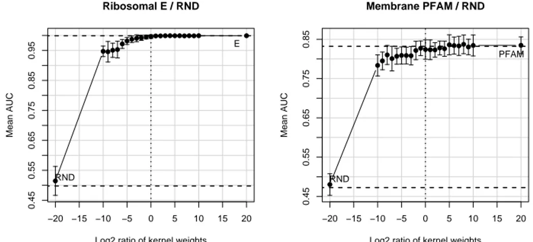
Figure 2: The figure plots the mean AUC and standard errors when varying the relative ratio log₂(µ_E/µ_RND), where µ_Eand µ_RNDare the weights assigned to the expression kernel K_Eand the random kernel KRND.

−20 −15 −10 −5 0 5 10 15 20 0.45 0.55 0.65 0.75 0.85 0.95 Ribosomal E / RND

Log2 ratio of kernel weights

Mean AUC RND E −20 −15 −10 −5 0 5 10 15 20 0.45 0.55 0.65 0.75 0.85 Membrane PFAM / RND

Mean AUC

RND

PFAM

We carry on with an empirical analysis of the performance of the classifiers (ribosomal and membrane) when varying the ratio of the kernel weights.

The first experiment consists in analyzing the effect of adding a Gaussian noise kernel to the best kernel of each classification problem. In Figure 2 we see that the unweighted combination of the single kernel which leads to the best classifier with a random kernel does not influence the performance of the classifiers. The dashed lines denote the AUC level of the classifiers when using a single kernel (reported above and below the lines). Only when the random kernel has a weight 32 times higher than the best kernel the performances start dropping (albeit of a small quantity). This experiment confirms that the SVM is robust to Gaussian noise in the features.

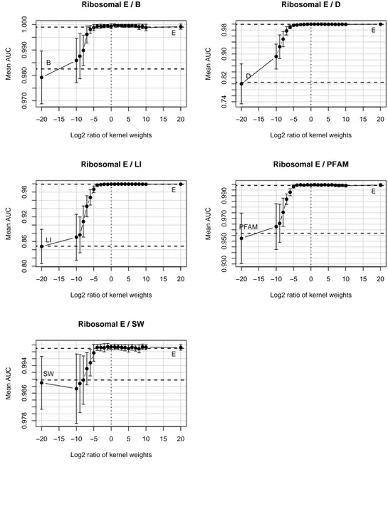
In the next experiment we consider the ribosomal problem and analyze the mean AUC when varying the relative ratio of the expression kernel with the other kernels. In Figure 3, we note that since the expression kernel is a very good kernel for the classification of the ribosomal proteins, then adding one of the other kernels has not effect on the resulting ROC score around zero (i.e. the unweighted sum, log₂ratio = 0).

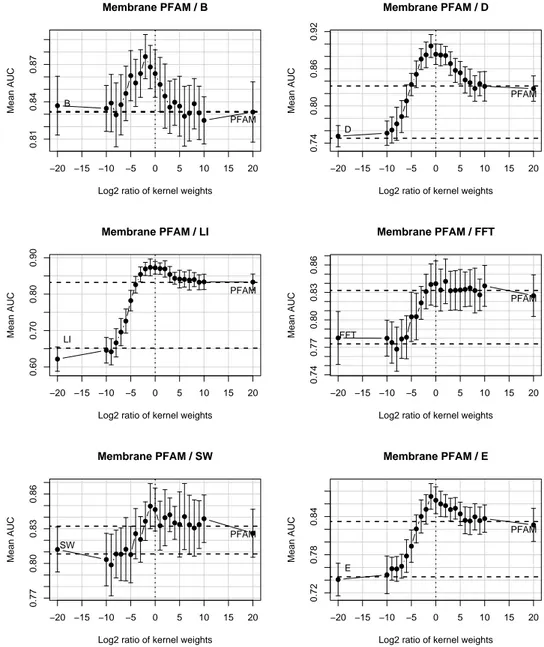
When analyzing the membrane problem the shape of the curves changes. In Figure 4 we plot the variation in the ROC score when adding to the PFAM kernel (the optimal single kernel for that problem) other kernels in different ratio. We can see that adding two different kernel can lead to an increase in the performance of the classifier.

The maximum of the curve is obtained very close to the ratio of zero (unweighted sum of kernels) and the ROC score near the edge of the plot tends to the respective single kernel performance. Only in the plot relative to the kernel KB the maximum seems to be shifted

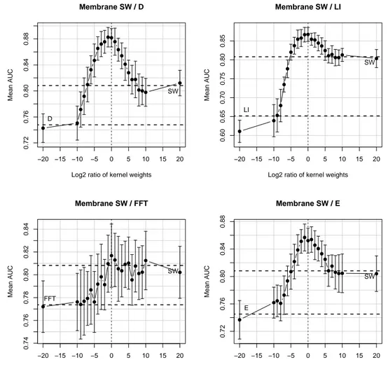
to the left (notice, however, that within the standard error the AUC values are comparable). This tendency is confirmed in Figure 5, where the reference kernel is K_B. In some plots, the maximum is shifted to the right (especially in the B/FFT plot), but considering the standard errors the variation in the ROC score is minimal. In the analysis of the plots in Figure 6 the trend is always the same, a maximum near or at the ratio equal to zero.

(14)

Figure 3: Variation in the AUC score when to the expression kernel is added one of the other kernels. −20 −15 −10 −5 0 5 10 15 20 0.970 0.980 0.990 1.000 Ribosomal E / B

Mean AUC B E −20 −15 −10 −5 0 5 10 15 20 0.74 0.82 0.90 0.98 Ribosomal E / D

Mean AUC D E −20 −15 −10 −5 0 5 10 15 20 0.80 0.86 0.92 0.98 Ribosomal E / LI

Mean AUC _LI E −20 −15 −10 −5 0 5 10 15 20 0.930 0.950 0.970 0.990 Ribosomal E / PFAM

Mean AUC PFAM E −20 −15 −10 −5 0 5 10 15 20 0.978 0.986 0.994 Ribosomal E / SW

Mean AUC

SW

(15)

Figure 4: Membrane problem. Variation in the AUC score when to the PFAM kernel is added one of the other kernels.

−20 −15 −10 −5 0 5 10 15 20

0.81

0.84

0.87

Membrane PFAM / B

Mean AUC B PFAM −20 −15 −10 −5 0 5 10 15 20 0.74 0.80 0.86 0.92 Membrane PFAM / D

Mean AUC D PFAM −20 −15 −10 −5 0 5 10 15 20 0.60 0.70 0.80 0.90 Membrane PFAM / LI

Mean AUC _LI PFAM −20 −15 −10 −5 0 5 10 15 20 0.74 0.77 0.80 0.83 0.86 Membrane PFAM / FFT

Mean AUC FFT PFAM −20 −15 −10 −5 0 5 10 15 20 0.77 0.80 0.83 0.86 Membrane PFAM / SW

Mean AUC SW PFAM −20 −15 −10 −5 0 5 10 15 20 0.72 0.78 0.84 Membrane PFAM / E

Mean AUC

E

(16)

Figure 5: Variation in the AUC score when to the B kernel is added one of the other kernels. −20 −15 −10 −5 0 5 10 15 20 0.72 0.78 0.84 0.90 Membrane B / D

Mean AUC D B −20 −15 −10 −5 0 5 10 15 20 0.60 0.70 0.80 0.90 Membrane B / LI

Mean AUC _LI B −20 −15 −10 −5 0 5 10 15 20 0.74 0.78 0.82 0.86 Membrane B / FFT

Mean AUC FFT B −20 −15 −10 −5 0 5 10 15 20 0.78 0.81 0.84 0.87 Membrane B / SW

Mean AUC SW B −20 −15 −10 −5 0 5 10 15 20 0.72 0.76 0.80 0.84 0.88 Membrane B / E

Mean AUC

E

(17)

Figure 6: Variation in the AUC score when to the SW kernel is added one of the other kernels. −20 −15 −10 −5 0 5 10 15 20 0.72 0.76 0.80 0.84 0.88 Membrane SW / D

Mean AUC D SW −20 −15 −10 −5 0 5 10 15 20 0.60 0.65 0.70 0.75 0.80 0.85 Membrane SW / LI

Mean AUC LI SW −20 −15 −10 −5 0 5 10 15 20 0.74 0.76 0.78 0.80 0.82 0.84 Membrane SW / FFT

Mean AUC _FFT SW −20 −15 −10 −5 0 5 10 15 20 0.72 0.76 0.80 0.84 0.88 Membrane SW / E

Mean AUC

E

(18)

and normalized (i.e. projected on the unit hypersphere) renders the unweighted sum of kernel the best choice for integration.

5 Conclusions

In this paper we proposed a novel method for integrating different data sets based on the entropy of kernel matrices. We show that von Neumann entropy correlates with the classifi-cation performances of different kernels on bioinformatics data sets and thus we used entropy to assign the weights of different and heterogeneous kernels in a simple kernel integration scheme. Our method is considerably less computationally expensive than the semi-definite approach, involving only the computation of a function of the eigenvalues of the kernel ma-trices and, differently from existing approaches, the computational complexity is only linear with the number of kernels. Moreover our method is independent from the labels of the sam-ples and from the learning process, two characteristics that makes it suitable for a wide range of kernel methods, whereas the use of label restricts the application domain to supervised classification. The results obtained on SVM classification are equivalent to those derived us-ing the semi-definite approach and, surprisus-ingly, to those achieved usus-ing a simple unweighted sum of kernels.

This conclusion agrees with the conclusion derived in a recent paper [Lewis et al., 2006], where a study on the performance of the SVM on the task of inferring gene functional annota-tions from a combination of protein sequences and structure data is carried out. The authors stated that the unweighted combination of kernels performed better, or equally, than the more complex weighted combination using the semi-definite approach and that larger data sets might benefit from a weighted combination.

However, as analyzed here, even when the number of data set is higher (six in one problem and seven in the other) still the unweighted sum of kernels gives performance similar to the weighted ones. Moreover, as a further investigation, we empirically showed that when considering the sum of pairs of kernels, the integration of such kernels was beneficial and the maximum of performance are obtained with the unweighted sum of kernels.

References

S.F. Altschul, W. Gish, W. Miller, E.W. Myers, and D.J. Lipman. Basic local alignment search tool. Journal of Molecular Biology, 215(3):403–410, 1990.

Kristin P. Bennett and Ayhan Demiriz. Semi-supervised support vector machines. In Advances in Neural Information Processing Systems, pages 368–374. MIT Press, 1998.

O. Chapelle, J. Weston, and B. Schlkopf. Cluster kernels for semi-supervised learning. In S. Becker, S. Thrun, and K. Obermayer, editors, NIPS 2002, volume 15, pages 585–592, Cambridge, MA, USA, 2003. MIT Press.

C. Cortes and V. Vapnik. Support-vector networks. Mach Learn, 20(3):273–297, 1995. T. De Bie, K. Arenberg, and N. Cristianini. Convex Methods for Transduction. In Advances in

Neural Information Processing Systems 16: Proceedings of the 2003 Conference. Bradford Book, 2004.

(19)

A. Elisseeff and J. Weston. A Kernel Method for Multi-Labelled Classification. Advances in Neural Information Processing Systems, 1:681–688, 2002.

T.S. Furey, N. Cristianini, N. Duffy, D.W. Bednarski, M. Schummer, and D. Haussler. Sup-port vector machine classification and validation of cancer tissue samples using microarray expression data, 2000.

M. Girolami. Mercer kernel-based clustering in feature space. Neural Networks, IEEE Trans-actions on, 13(3):780–784, May 2002. ISSN 1045-9227. doi: 10.1109/TNN.2002.1000150. M. Girolami and M. Zhong. Data integration for classification problems employing gaussian

process priors. In B. Scholkopf, J. C. Platt, and T. Hofmann, editors, Advances in Neural Information Processing Systems 19. MIT Press, Cambridge, MA, 2007. To appear.

R.I. Kondor and J. Lafferty. Diffusion kernels on graphs and other discrete structures. In Proceedings of the ICML, 2002.

J. Kyte and RF Doolittle. A simple method for displaying the hydropathic character of a protein. Journal of Molecular Biology, 157(1):105–32, 1982.

G. R. G. Lanckriet, T. De Bie, N. Cristianini, M. I. Jordan, and W. S. Noble. A statistical framework for genomic data fusion. Bioinformatics, 20(16):2626–2635, 2004a.

G. R. G. Lanckriet, M. Deng, N. Cristianini, M. I. Jordan, and W. S. Noble. Kernel-based data fusion and its application to protein function prediction in yeast. In Proceedings of the Pacific Symposium on Biocomputing (PSB), Big Island of Hawaii, Hawaii, 2004b. Darrin P. Lewis, Tony Jebara, and William Stafford Noble. Support vector machine

learn-ing from heterogeneous data: an empirical analysis uslearn-ing protein sequence and structure. Bioinformatics, 22(22):2753–2760, 2006.

Andrea Malossini, Enrico Blanzieri, and Raymond T. Ng. Detecting potential labeling errors in microarrays by data perturbation. Bioinformatics, 22(17):2114–2121, 2006. doi: 10. 1093/bioinformatics/btl346.

S. Mika, G. Ratsch, J. Weston, B. Scholkopf, and KR Mullers. Fisher discriminant analysis with kernels. In Neural Networks for Signal Processing IX, 1999. Proceedings of the 1999 IEEE Signal Processing Society Workshop, pages 41–48, 1999a.

S. Mika et al. Fisher discriminant analysis with kernels. In Y.-H Hu, E. Larsen, J.and Wilson, and Dougglas S., editors, Neural Networks for Signal Processing, pages 41–48. IEEE, 1999b. M. Nielsen and I. Chuang. Quantum Computation and Quantum Information. Cambridge

University Press, Cambridge UK, 2000.

P. Pavlidis, T. S. Furey, M. Liberto, D. Haussler, and W. N. Grundy. Promoter region-based classification of genes. In Proceedings of the Pacific Symposium on Biocomputing, pages 151–163, River Edge, NJ, 2001a. World Scientific.

P. Pavlidis, J. Weston, J. Cai, and W. N. Grundy. Gene functional classification from heteroge-neous data. In Proceedings of the Fifth Annual International conference on Computational Biology (RECOMB), pages 249–255, New York, 2001b. ACM Press.

(20)

P. Pavlidis, J. Weston, J. Cai, and W. S. Noble. Learning gene functional classifications from multiple data types. Journal of Computational Biology, 9(2):401–411, 2002.

R.E. Schapire and Y. Singer. BoosTexter: A Boosting-based System for Text Categorization. Machine Learning, 39(2):135–168, 2000.

B. Sch¨olkopf and A.J. Smola. Learning with Kernels: Support Vector Machines, Regulariza-tion, OptimizaRegulariza-tion, and Beyond. MIT Press, 2002a.

B. Sch¨olkopf and J. Smola. Learning with kernels. MIT Press, Cambridge, MA, 2002b. B. Sch¨olkopf, K. Tsuda, and J.P. Vert. Kernel Methods in Computational Biology. Bradford

Books, 2004.

Bernhard Sch¨olkopf, Alexander J. Smola, and Klaus-Robert M¨uller. Kernel principal compo-nent analysis. In Advances in kernel methods: support vector learning, pages 327–352. MIT Press, Cambridge, MA, USA, 1999.

J. Shawe-Taylor and N. Cristianini. Kernel Methods for Pattern Analysis. Cambridge Uni-versity Press New York, NY, USA, 2004.

T.F. Smith and M.S. Waterman. Identification of common molecular subsequences. Journal of Molecular Biology, 147(1):195–7, 1981.

A.J. Smola and B. Sch¨olkopf. A tutorial on support vector regression. Statistics and Com-puting, 14(3):199–222, 2004.

S. Sonnenburg, G. Rätsch, and C. Schäfer. A General and Efficient Multiple Kernel Learning Algorithm. Advances in Neural Information Processing Systems, pages 1273–1280, 2006a. S. Sonnenburg, G. Rätsch, C. Schäfer, and B. Schölkopf. Large Scale Multiple Kernel

Learn-ing. The Journal of Machine Learning Research, 7:1531–1565, 2006b.

E.L.L. Sonnhammer, S.R. Eddy, and R. Durbin. Pfam: A comprehensive database of protein domain families based on seed alignments. Proteins Structure Function and Genetics, 28 (3):405–420, 1997.

K. Tsuda, S. Akaho, and K. Asai. The EM algorithm for kenel matrix completation with auxiliary data. Journal of Machine Learning Research, 4:67–81, 2003.

K. Tsuda, S. Uda, T. Kin, and K. Asai. Minimizing the cross validation error to mix kernel matrices of heterogeneous biological data. Neural Processing Letters, 19:63–72, 2004. H. Valizadegan and R. Jin. Generalized Maximum Margin Clustering and Unsupervised

Kernel Learning. Advances in Neural Information Processing Systems, pages 1417–1424, 2007.

L. Vandenberghe and S. Boyd. Semidefinite programming. SIAM Review, 38(1):49–95, 1996. V.N. Vapnik. The Nature of Statistical Learning Theory. Springer, 2000.

(21)

J-P. Vert and M. Kanehis. Graph-driven features extraction from microarray data using diffusion kernels and kernel CCA. In S. Becker, S. Thrun, and K. Obermayer, editors, Advances in Neural Information Processing Systems, volume 15, pages 1425–1432. MIT Press, Cambridge, MA, 2003.

Z. Wang, S. Chen, and T. Sun. MultiK-MHKS: A Novel Multiple Kernel Learning Algorithm. IEEE Transactions on Pattern Analysis and Machine Intelligence, 30(2):348–353, 2008. J. Weston, C. Leslie, E. Ie, D. Zhou, A. Elisseeff, and W.S. Noble. Semi-supervised protein

classification using cluster kernels. Bioinformatics, 21(15):3241–3247, 2005.

L. Xu and D. Schuurmans. Unsupervised and semi-supervised multi-class support vector machines. In Proceedings of the National Conference on Artificial Intelligence, volume 20, page 904. Menlo Park, CA; Cambridge, MA; London; AAAI Press; MIT Press; 1999, 2005. L. Xu, J. Neufeld, B. Larson, and D. Schuurmans. Maximum margin clustering. Advances in

Neural Information Processing Systems, 17:1537–1544, 2005.

Y. Yamanishi, J-P. Vert, and M. Kanehisa. Protein network inference from multiple genomic data: a supervised approach. Bioinformatics, 20(Suppl. 1):i363–i370, 2004.

Ying Zhao, Jian pei Zhang, and Jing Yang. The model selection for semi-supervised sup-port vector machines. Internet Computing in Science and Engineering, 2008. ICICSE ’08. International Conference on, pages 102–105, Jan. 2008. doi: 10.1109/ICICSE.2008.29.