Overcoming uncertainty and the curse of dimensionality in data clustering

(1)

(2)

(3)

Acknowledgments

Several people have contributed to allow this thesis to exist.

I acknowledge my advisor, prof. Sergio Greco, for the guidance over these years and the opportunity to carry on the research of this thesis without constraining it.

I would like to thank the two people who shared with me much more time than anyone else: my “de facto” second advisor Andrea Tagarelli and my roommate Giovanni “Gianni” Ponti.

Thanks to the “UNICZ team”, Pierangelo Veltri, Giuseppe Tradigo, and Mario Cannataro. Besides the collaboration in some works, they have the great merit to have made the days spent in the “wonderful” Catanzaro better days!

I am grateful to Carlotta Domeniconi for the chance to experience the US, and, along with Sean Luke and Roberto Avogadri, for having made such an experience nice and homely.

I cannot forget all the people who, during these years, “housed” the fifth floor of the 41C cube: who was here before my arrival and is still here right now (Andrea, Bettina, Cristian, who they call “Cristiano”, Filippo, Francesco, Irina, Lillo, Sergio), who was here but has been “unfaithful” and moved to higher or lower floors (Ester, Luciano, Massimo), and the “new entries” (An-drea, Francesca, Giuseppe). Among them, a special thank goes to Giovanni Costabile for having tolerated and satisfied me in every my “technical re-quest”!

Finally, I am going to conclude by writing a sentence which, I am sure, has not ever previously ended any acknowledgment section: LAST BUT NOT LEAST, I want to thank my best friends and, in particular, my family: thanks mum, thanks dad, thanks Rita!

(4)

(5)

(6)

(7)

Abstract

Uncertainty and the curse of dimensionality are two crucial problems that usually affect data clustering.

Uncertainty in data clustering may be typically considered at data level or clustering level. Data level uncertainty is inherently present in the repre-sentation of several kinds of data objects from various application contexts (e.g., sensor networks, moving objects databases, biomedicine). This kind of uncertainty should be carefully taken into account in a clustering task in order to achieve adequate accuracy; unfortunately, traditional clustering methods are designed to work only on deterministic vectorial representations of data objects. Clustering uncertainty is related to the output of any clustering algo-rithm. Indeed, the ill-posed nature of clustering leads to clustering algorithms that cannot be generally valid for any input dataset, i.e., their output results are necessarily uncertain. Clustering ensembles has been recognized as a pow-erful solution to overcome clustering uncertainty. It aims to derive a single clustering solution (i.e., the consensus partition) from a set of clusterings rep-resenting different partitions of the same input dataset (i.e., the ensemble). A major weakness of the existing clustering ensembles methods is that they compute the consensus partition by equally considering all the solutions in the ensemble.

The curse of dimensionality in data clustering concerns all the issues that naturally arise from data objects represented by a large set of features and are responsible of poor accuracy and efficiency achieved by traditional clustering methods working on high dimensional data. Classic approaches to the curse of dimensionality include global and local dimensionality reduction. Global techniques aim at reducing the dimensionality of the input dataset by applying the same algorithm(s) to all the input data objects. Local dimensionality reduction acts by considering subsets of the input dataset and performing dimensionality reduction specific for any of such subsets. Projective clustering is an effective class of methods falling into the category of local dimensionality reduction. It aims to discover clusters of objects along with the corresponding subspaces, following the principle that objects in the same cluster are close to each other if and only if they are projected onto the subspace associated to that cluster.

(8)

viii Abstract

The focus of this thesis is on the development of proper techniques for overcoming the crucial problems of uncertainty and the curse of dimension-ality arising from data clustering. This thesis provides the following main contributions.

Uncertainty. Uncertainty at a representation level is addressed by proposing:

UK-medoids, which is a new partitional algorithm for clustering un-certain objects, which is designed to overcome efficiency and accuracy issues of some existing state-of-the-art methods;

U-AHC, i.e., the first (agglomerative) hierarchical algorithm for clus-tering uncertain objects;

a methodology to exploit U-AHC for clustering microarray biomedical data with probe-level uncertainty.

Clustering uncertainty is addressed by focusing on the problem of weighted consensus clustering, which aims to automatically determine weighting schemes to discriminate among clustering solutions in a given ensemble. In particular:

three novel diversity-based, general schemes for weighting the individ-ual clusterings in a given ensemble are proposed, i.e., Single-Weighting (SW), Group-Weighting (GW), and Dendrogram-Weighting (DW);

three algorithms, called WICE, WCCE, and WHCE, are defined to eas-ily involve clustering weighting schemes into any clustering ensembles algorithm falling into one of the main classes of clustering ensembles approaches, i.e., instance-based, cluster-based, and hybrid.

The curse of dimensionality. Global dimensionality reduction is addressed by focusing on the time series data application context:

the Derivative time series Segment Approximation (DSA) model is proposed as a new time series dimensionality reduction method de-signed for accurate and fast similarity detection and clustering;

Mass Spectrometry Data Analysis (MaSDA) system is presented; it mainly aims at analyzing mass spectrometry (MS) biomedical data by exploiting DSA to model such data according to a time series-based representation;

DSA is exploited for profiling low-voltage electricity customers. Regarding local dimensionality reduction, a unified view of projective clus-tering and clusclus-tering ensembles is provided. In particular:

the novel Projective Clustering Ensembles (PCE) problem is addressed and formally defined according two specific optimization formulations, i.e., two-objective PCE and single-objective PCE ;

MOEA-PCE and EM-PCE algorithms are proposed as novel heuristics to solve two-objective PCE and single-objective PCE, respectively. Absolute accuracy and efficiency performance achieved by the proposed techniques, as well as the performance with respect to the prominent state-of-the-art methods are evaluated by performing extensive sets of experiments on benchmark, synthetically generated, and real-world datasets.

(9)

List of Tables

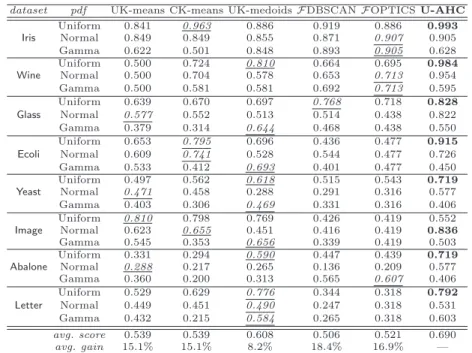
4.1 UK-Medoids vs. competing methods: clustering quality results (F1-Measure) . . . 46

5.1 U-AHC vs. competing methods: accuracy results (F1-Measure) for univariate models . . . 71

5.2 U-AHC vs. competing methods: accuracy results (F1-Measure) for multivariate models . . . 71

5.3 Accuracy results of U-AHC in clustering microarray data

(cophenetic coefficient) . . . 76

7.1 Evaluating SW, GW, and DW clustering weighting schemes: (a) Glass, and (b) Ecoli . . . 98

7.2 Evaluating SW, GW, and DW clustering weighting schemes: (a) ImageSegmentation, and (b) ISOLET . . . 99

7.3 Evaluating SW, GW, and DW clustering weighting schemes: LetterRecognition . . . .100

7.4 Evaluating SW, GW, and DW clustering weighting schemes: (a) Tracedata, and (b) ControlChart . . . .101

9.1 Segmentation and compression using DSA . . . .119

9.2 DSA vs. competing methods: avg quality results (F1-Measure) for K-Means . . . .123

9.3 DSA vs. competing methods: quality results (F1-Measure) for UPGMA . . . .124

9.4 DSA vs. competing methods: best time performances (msecs) in time series modeling . . . .125

9.5 DSA vs. competing methods: summary of best time

performances (msecs) in time series modeling and clustering . . .128

10.1 Evaluating MaSDA system: summary of clustering results on the various test datasets . . . .144

(16)

xvi List of Tables

10.2 Clustering load profile data: best (average) performance on

Weekdays load profiles . . . .155

10.3 Clustering load profile data: best (average) performance on Saturdays load profiles . . . .155

10.4 Clustering load profile data: best (average) performance on Sundays/holidays load profiles . . . .156

12.1 MOEA-PCE and EM-PCE: similarity results w.r.t. reference classification (object-based representation) . . . .180

12.2 MOEA-PCE and EM-PCE: similarity results w.r.t. reference classification (feature-based representation) . . . .180

12.3 MOEA-PCE and EM-PCE: average similarity results w.r.t. ensemble . . . .181

12.4 MOEA-PCE and EM-PCE: error rate results . . . .181

A.1 UCI benchmark datasets used in the experiments . . . .187

A.2 Time Series datasets used in the experiments . . . .188

A.3 Microarray datasets used in the experiments . . . .189

A.4 Mass spectrometry datasets used in the experiments . . . .189

B.1 Average approximation errors on derivative estimation: DDTW model vs. DSA model. Each function is valued on 101 points over the range [−5, +5]. . . .192

B.2 DDTW-based clustering results by varying the derivative estimation model . . . .193

B.3 DSA-based clustering results by varying the derivative estimation model . . . .193

C.1 Time series clustering: K-Means performance reduction in case of no smoothing . . . .196

C.2 Summary of the preprocessing setups providing the best time series clustering results by K-Means . . . .196

(17)

List of Figures

1.1 The Knowledge Discovery in Databases (KDD) process . . . 4

1.2 An example of time series data . . . 7

1.3 Three clusters existing in different subspaces . . . 9

2.1 A taxonomy of clustering approaches . . . 16

2.2 A dendrogram showing a possible cluster hierarchy built upon a simple dataset of 16 data objects . . . 22

3.1 Graphical representation of (a) a multivariate uncertain object and (b) a univariate uncertain object . . . 36

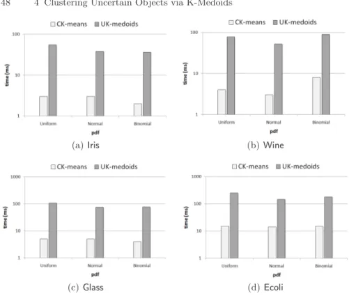
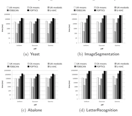
4.1 UK-Medoids vs. competing methods: clustering time performances . . . 47

4.2 UK-Medoids vs. CK-Means: performance of the algorithm runtimes (pre-computing phases are ignored) . . . 48

5.1 U-AHC vs. competing methods: clustering time performances in the univariate model . . . 73

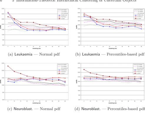
5.2 Accuracy results of U-AHC and competing methods in clustering microarray data (quality) . . . 76

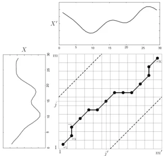
8.1 An example warping path . . . .106

8.2 Two time series aligned according to (a) Euclidean norm and (b) DTW . . . .106

9.1 Sample instances from the test datasets used for evaluating DSA performance. One time series from each class is displayed for each dataset . . . .118

9.2 DSA vs. competing methods: time performances in time series modeling and clustering (GunX, Tracedata, ControlChart, CBF) .126

(18)

xviii List of Figures

9.3 DSA vs. competing methods: time performances in time series modeling and clustering (Twopat, Mixed-BagShapes,

OvarianCancer) . . . .127

10.1 The overall conceptual architecture of the MaSDA system . . . . .134

10.2 A sample screenshot of the MaSDA system for MS preprocessing135

10.3 MSPTool preprocessing wizard - summary of the preprocessing settings . . . .136

10.4 Peak smoothing: (a) example M-peaks and (b) the

corresponding ideal peak; (c) three local M-peaks and (d) the resulting profile after smoothing . . . .138

10.5 A screenshot of the MaSDA tool for clustering MS data . . . .140

10.6 An example of data summarization: (a) a set of time series

and (b) the computed prototype . . . .141

10.7 Evaluating MaSDA system—clustering quality results (F1-Measure on the left, Entropy on the right): (a) Cardiotoxicity, (b) Pancreatic, and (c) Prostate . . . .143

10.8 Evaluating MaSDA system—clusters vs. natural classes from Prostate: (a) cluster and (b) class of cancer with PSA>10 ng/ml; (c) cluster and (d) class of no evidence of

disease . . . .145

10.9 Evaluating MaSDA system on OvarianCancer dataset: on top, raw spectra of (a) control class and (b) diseased class; on bottom, preprocessed spectra of (c) control class and (d) diseased class . . . .147

10.10The Enel Telegestore architecture . . . .150

10.11A snapshot of the Exeura Rialto suite for data mining . . . .154

10.12Distribution of weekdays load profiles over clusters obtained by TS-Part with DTW . . . .156

11.1 Some projective clusters existing in arbitrarily-oriented

subspaces . . . .160

B.1 Approximation errors on derivative estimation: DDTW model vs. DSA model . . . .192

(19)

Part I

(20)

(21)

1 Introduction

1.1 Knowledge Discovery in Databases, Data Mining,

Clustering

Knowledge Discovery in Databases (KDD) is the non-trivial process of identifying novel, valid, potentially useful, and ultimately understandable pat-terns in data [FPS96]. The term “pattern” refers to a subset of the data ex-pressed in some language or a model exploited for representing such a subset. KDD aims to discover patterns that (i) do not result in straightforwardly computing predefined quantities (i.e., non-trivial), (ii) can apply to new data with some degree of certainty (i.e., valid), (iii) are previously unknown (i.e., novel), (iv) provide some benefit to the user or further task (i.e., potentially useful), and (v) lead to insight, immediately or after some post-processing (i.e., understandable).

The KDD process is an iterative and interactive sequence of the following main steps (Fig. 1.1):

selection, whose main goal is to create a target data set from the orig-inal data, i.e., selecting a subset of variables or data samples, on which discovery has to be performed;

preprocessing, which aims to “clean” data by performing various opera-tions, such as noise modeling and removal, defining proper strategies for handling missing data fields, accounting for time sequence information;

transformation, which is responsible of reducing and projecting the data, in order to derive a representation suitable for the specific task to be per-formed; it is typically accomplished by involving transformation techniques or methods that are able to find invariant representations for the data;

data mining, which deals with extracting the interesting patterns by choos-ing (i) a specific data minchoos-ing method or task (e.g, summarization, classifi-cation, clustering, regression, and so on), (ii) the proper algorithm(s) for performing the task at hand, and (iii) the appropriate representation for the output results;

(22)

4 1 Introduction

Fig. 1.1. The Knowledge Discovery in Databases (KDD) process

interpretation/evaluation, which is exploited by the user to interpret and extract knowledge from the mined patterns, by visualizing the patterns; this interpretation is typically carried out by visualizing the patterns, the models, or the data given such models and, in case, iteratively looking back at the previous steps of the process.

Data mining represents the “core” step of the KDD process, so much so that the “data mining” and “KDD” terms are often treated as syn-onyms [HK01]. Data mining tasks are classified into predictive and descrip-tive [FPSU96]. Predicdescrip-tive tasks refer to building a model useful for predicting future behavior or values for certain features. These comprise association anal-ysis, i.e., discovering association rules that show attribute-value conditions occurring frequently together in a given set of data; classification and predic-tion, i.e., deriving some models (or functions) which describe data classes or concepts by a set of data objects whose class label is known (i.e., the training set); such models have the main goal of being used to predict the class of objects whose class label is unknown as accurately as possible; deviation de-tection, i.e., dealing with deviations in data, which are defined as differences between measured values and corresponding references such as previous values or normative values; evolution analysis, i.e., detecting and describing regular patterns in data whose behavior changes over time. On the other hand, in a descriptive data mining task, the model built has to describe the data in an understandable, effective, and efficient form. Relevant examples of descriptive tasks are data characterization, whose main goal is to summarize the general characteristics or features of a target class of data, data discrimination, i.e., a comparison of the general features of target class data objects with the general features of objects from one or a set of contrasting classes, and clustering.

Given a set of data objects, clustering aims to identify a finite set of groups of objects, i.e., clusters, so that the objects within the same cluster are

(23)

“sim-1.2 Uncertainty 5

ilar” to each other, whereas the objects belonging to different clusters are “dissimilar”. The degrees of (dis)similarity among data objects are computed and evaluated according to a similarity/distance measure that can be either specified by the user or inherently employed in the specific clustering algo-rithm. In a clustering task, there is no prior knowledge of the class labels associated to the objects to be grouped; according to this feature, clustering is often also referred to as unsupervised classification, to emphasize the dif-ference with respect to the (supervised) classification task, in which the class labels of the objects in the training set are known.

A large number of clustering algorithms has been proposed in the liter-ature [JD88, KR90]. Traditionally, these algorithms share to each other the following main features: (i) they work on a set of a data objects which are de-scribed according to a “deterministic” vectorial representation, i.e., as tuples of attribute or feature values; (ii) they assume and, consequently, guarantee high performances only if the number of features describing each data ob-ject is sufficiently small; (iii) they make the final decision about the output result without taking into account additional information, possibly given by, e.g., varying parameters and features and/or exploiting different algorithms or similarity measures. Unfortunately, due to recent advances in database appli-cations which lead to a significant increasing of the complexity of the data to be treated, the above features make the traditional clustering algorithms not easily applicable to a lot of newly emerged application contexts. Within this view, major challenges in data clustering are focusing on overcoming issues related to the crucial notions of uncertainty and the curse of dimensionality.

1.2 Uncertainty

Uncertainty in Data Representation. Handling uncertainty in data management has been recently requiring more and more importance in a wide range of application contexts [Agg09]. Data uncertainty naturally arises from, e.g., implicit randomness in a process of data generation/acquisition, impre-cision in physical measurements, application of approximation methods, and data staling. This makes uncertainty inherently present in several application domains. For instance, sensor measurements may be imprecise at a certain degree due to the presence of various noisy factors (e.g., signal noise, in-strumental errors, wireless transmission) [CLL06, CKP03]. To address this issue, it is advisable to model sensor data as continuous probability distri-butions [FGB02, DGM+_{05]. Another example is given by data representing} moving objects, which continuously change their location so that the exact positional information at a given time instant may be unavailable [LHY04]. Moreover, some methods have recently been defined to handle uncertainty in gene expression data [MFNL03, HRC+_{05, LMLR05]. Further examples come} from distributed applications, privacy preserving data mining, and forecasting or other statistical techniques used to generate data attributes [AY09].

(24)

6 1 Introduction

Dealing with uncertain data has raised several issues in data manage-ment and knowledge discovery. In particular, clustering uncertain data is especially challenging and has been attracting increasing interest in recent years [KP05a, KP05b, CCKN06, NKC+_{06, S. 07, KLC}+_{08]. Indeed, in order} to produce meaningful results, uncertain data clustering algorithms have to necessarily deal with the non-trivial issue of carefully considering and model-ing uncertainty. This represents a crucial point, because, if data uncertainty is not effectively taken into account and represented, any clustering algorithm may probably fail in discovering accurate cluster structures.

Clustering Uncertainty. Clustering is typically affected by a different kind of uncertainty, i.e., clustering uncertainty, which is somehow related to the output results. Clustering uncertainty is mainly motivated by the “ill-posed” nature of clustering: it is well-known that there do not exist defi-nitely best algorithms, similarity measures, and parameter settings for pro-viding general valid solutions to the clustering problem [JMF99]. Instead, such choices have to be made depending on the specific data to be clustered. Within this view, any clustering result outputted by a clustering algorithm equipped with a specific similarity measure and parameter values cannot be recognized as “certain”; rather, many different configurations of algorithm, similarity measure, and parameter setting that lead to different output re-sults (and, hence, to uncertainty in clustering rere-sults) should be in principle taken into account.

Clustering ensembles [SG02], also known as consensus clustering or aggre-gation clustering, has recently emerged as a powerful tool to face the issues due to uncertainty in clustering results. In particular, clustering ensembles aims to make a clustering solution more robust against the bias due to the peculiarities of the specific clustering algorithm. Basically, clustering ensem-bles resorts to the idea of combining multiple classifiers, which has received increased attention in the last years [BK99]. Given a data collection, a set of clustering solutions, or ensemble, can be generated by varying one or more as-pects, such as the clustering algorithm, the parameter setting, and the number of features, objects or clusters. Given an ensemble, a major goal is to extract a consensus partition, i.e., a clustering solution that maximizes some objec-tive function (the consensus function) defined by taking into account different information available from the given set of clustering solutions.

1.3 The Curse of Dimensionality

The term “curse of dimensionality”, as originally coined in [Bel61], refers to the impossibility of optimizing a function of many variables by a brute force search on a discrete multidimensional grid [SEK04]. However, in data management, the curse of dimensionality is more generally referred to all the accuracy and efficiency issues due to high dimensional data, i.e., data

(25)

1.3 The Curse of Dimensionality 7

Fig. 1.2. An example of time series data

whose representation is given by a large number of variables (i.e, features). Major issues arising from the curse of dimensionality concern the sparsity of data represented in high dimensional spaces and the meaningfulness of the distance measure applied to this kind of data. Indeed, it has been shown that, for certain data distributions, the relative distances of the closest and farthest data points of an independently selected point goes to zero as the dimensionality increases [BGRS99]; a similar result involving the absolute distances and the Lpnorm (p ≥ 3) has been proved in [HAK00]. Such results make the curse of dimensionality phenomenon particularly critical especially in a task of clustering, since it is well-known that clustering puts its basis on the notion of similarity/distance between data objects.

Nowadays, high dimensional data arise from a lot of various application domains. Relevant examples are biomedical data, text data, data managed by e-commerce applications, web data, xml and semistructured data, time series data. In particular, time series, i.e., sequences of (real) numeric values upon which a total order based on timestamps is defined, are generally used to rep-resent the temporal evolution of objects (cf. Fig. 1.21_{). To this purpose,} man-aging time series data by means of data mining techniques, and, in particular, clustering, is challenging due to the enormous amounts of such data naturally available from several sources of different domains, e.g., speech recognition, financial and market data analysis, telecommunication and telemetry, sensor networking, motion tracking, meteorology [WY05, Lia05].

Global Dimensionality Reduction. A well-known class of methods and algorithms which aim to alleviate the issues arising from high dimensional data is the so-called dimensionality or dimension reduction [Fod02]. The main goal of dimensionality reduction is to compute, for each data object having m dimensions (i.e., represented by a number of features equal to m), a different

(26)

8 1 Introduction

representation given by m0 _{features, where m}0 _{¿ m. The new m}0_-dimensional representation is typically carried out globally to the entire set of objects, i.e., the same algorithm or scheme is exploited for all the objects.

Dimensionality reduction techniques can be classified into two main cat-egories, namely domain-driven and general. Domain-driven techniques are specific and specialized only for the application context that are designed to; hence, they are not applicable or do not guarantee high performances when involved in more general scenarios. As an example, there has been proposed a lot of dimensionality reduction techniques for time series data [DTS+_08]. Al-though such techniques fulfill some crucial requirements arising from the time series application context, such as, e.g., time-warping awareness, they cannot be recognized as generally valid for different application domains. General di-mensionality reduction aims to define methods that are suitable for dealing with any kind of data. General techniques comprise feature selection [MBN02] and feature extraction [GGNZ06]. According to feature selection, the dimen-sionality is reduced by selecting a subset of the original features of the data objects, while discarding the remaining ones. The crucial problem of choosing the features to be maintained can be solved by taking into account differ-ent criteria. For instance, according to wrapper models [KJ97, KSM00], the relevant features are selected by evaluating the results obtained by running one or more clustering algorithms on the reduced space. Entropy-based crite-ria [DLY97, DCSL02] involve the evaluation of the entropy of the distribution of the feature values in each dimension. On the other hand, feature extraction methods construct a new, smaller set of features by exploiting the information available from the original one. Well-established feature extraction techniques include Principal Component Analysis (PCA) [DH73, Fuk90, Jol02], which computes the new features as linear combinations of the original ones, and is a special case of a more general matrix decomposition method called Singular Value Decomposition (SVD) [Str88, Dep89, Sch91].

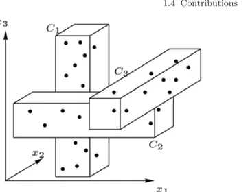
Local Dimensionality Reduction. In the context of data clustering, it may happen that any cluster to be discovered “exists” in a specific subspace, i.e., its objects are close to each other if (and only if) they are projected onto that subspace. Thus, performing dimensionality reduction globally to the entire set of objects may lead to meaningless clustering results. Indeed, global dimensionality reduction might eliminate or transform one o more dimensions that are potentially relevant to at least one cluster; also, since the subspaces associated to each cluster may be in general different to each other, the global reduced representation can be clearly not consistent with the subspaces of the various clusters. An illustrative example of this scenario is depicted in Fig. 1.3;2 _{the three clusters C}

1, C2, and C3 exist in the subspaces given by the sets of features {x1}, {x2}, and {x3}, respectively; therefore, the subspaces associated to each cluster are all different to each other and each dimension is relevant to at least one cluster.

(27)

1.4 Contributions 9

Fig. 1.3. Three clusters existing in different subspaces

Within this view, for a clustering task, it is advisable to perform a dimen-sionality reduction that is local to the single cluster. This is the main goal of subspace clustering and projective (or projected) clustering [PHL04, KKZ09], which aim to discover the cluster structure along with the subspaces corre-sponding to each cluster. As a consequence, subspace and projective clustering tend to be less noisy—because each group of data is represented over a sub-space which does not contain irrelevant or redundant dimensions—and more understandable—because the exploration of a cluster is much easier when only few dimensions are involved. Projective clustering and subspace cluster-ing problems are strictly related to each other.3 _{A major difference between} the two problems is that projective clustering outputs a single partition of the input set of data objects, whereas subspace clustering aims to find a set of clustering solutions, each one having clusters defined in a specific subspace. Indeed, subspace clustering algorithms typically aim to find clustering struc-tures in every possible “interesting” subspace.

1.4 Contributions

The focus of this thesis is on the crucial problems of uncertainty and the curse of dimensionality arising from data clustering. The main contributions of this thesis are summarized in the following.

Uncertainty. The problem of clustering data affected by uncertainty at a rep-resentation level is deeply investigated. In particular, main contributions in this respect include:

3 _{The terms “projective clustering” and “subspace clustering” are not used in a} unified way in the literature.

(28)

10 1 Introduction

UK-medoids: a new partitional algorithm for clustering uncertain data, which is designed to overcome efficiency and accuracy issues of some existing partitional uncertain data clustering algorithms;

U-AHC : the first (agglomerative) hierarchical algorithm for clustering uncertain data;

as a special case of uncertain data, the problem of clustering microarray biomedical data with probe-level uncertainty is addressed and solved by exploiting the U-AHC algorithm.

Clustering uncertainty is addressed from a clustering ensembles perspec-tive, i.e., by focusing on the problem of weighted consensus clustering, which aims to automatically determine weighting schemes to discriminate among clustering solutions in a given ensemble. In particular, contribu-tions of this thesis to clustering ensembles include:

Single-Weighting (SW), Group-Weighting (GW), and Dendrogram-Weighting (DW): three novel diversity-based, general schemes for weighting the individual clusterings in a given ensemble;

WICE, WCCE, and WHCE : three algorithms to easily involve cluster-ing weightcluster-ing schemes into any clustercluster-ing ensembles algorithm fallcluster-ing into one of the main classes of clustering ensembles approaches, i.e., instance-based, cluster-based, and hybrid.

The curse of dimensionality. Global dimensionality reduction is addressed by focusing on a domain-driven scenario; in particular, the application context taken into account is that of time series data. Contributions in this regard are the following:

Derivative time series Segment Approximation (DSA) model: a new time series dimensionality reduction method (i.e, representation model) designed for accurate and fast similarity detection and clustering of time series data;

Mass Spectrometry Data Analysis (MaSDA): a system for analyzing mass spectrometry biomedical data, whose core exploits DSA to model mass spectrometry data according to a time series-based representa-tion;

exploiting DSA for low-voltage electricity customer profiling.

Regarding local dimensionality reduction, the projective clustering and clustering ensembles problems are viewed for the first time as two faces of the same coin. In particular:

the novel Projective Clustering Ensembles (PCE) problem is inves-tigated and formally defined by providing two specific optimization formulations, i.e., two-objective PCE and single-objective PCE ;

MOEA-PCE and EM-PCE algorithms are proposed as novel heuristic solutions to the two-objective PCE and single-objective PCE prob-lems, respectively.

(29)

1.5 Outline of the Thesis 11

1.5 Outline of the Thesis

This thesis is organized in five parts:

Part I, Preliminaries, provides an introduction and the background to clustering data mining task;

Part II, Uncertainty in Data Clustering – data level, deals with the problem of uncertainty at a data representation level arising from data clustering;

Part III, Uncertainty in Data Clustering – clustering level, addresses the so-called clustering uncertainty, by focusing, in particular, on the problem of clustering ensembles;

Part IV, The Curse of Dimensionality in Data Clustering – global dimen-sionality reduction, focuses on global dimendimen-sionality reduction as a solution for overcoming the curse of dimensionality problem in data clustering;

Part V, The Curse of Dimensionality in Data Clustering – local dimension-ality reduction, deals with the curse of dimensiondimension-ality in data clustering from a local dimensionality reduction perspective; in particular, the focus is on the problem of projective clustering.

The five parts are articulated around the following chapters.

Chapter 1 informally describes the context of this thesis. It firstly intro-duces the KDD process, paying particular attention on data mining, as a major step of KDD, and clustering, i.e., the specific data mining task addressed in this thesis. Then, it provides an overview of the problems of uncertainty and the curse of dimensionality in data clustering, along with a brief summary of the main existing techniques for overcoming these problems. Finally, the main contributions and the outline of the thesis conclude the chapter.

Chapter 2 provides background notions to the clustering task in data min-ing. The focus of the chapter is on the algorithms/criteria needed for a clear explanation of the proposals discussed in the remainder of the thesis. It firstly overviews the main existing classes of clustering approaches, namely, parti-tional relocation, density-based, and hierarchical. Afterward, the problem of soft clustering is introduced, along with the cluster validity criteria aimed at assessing the quality of a clustering solution.

Chapter 3 deals with the problem of uncertainty in data representation, which is analyzed from a clustering perspective. It provides a background to the problem at hand. First, the main models used for representing data uncertainty are discussed, particularly focusing on the model adopted by the so-called uncertain objects, which are the specific kind of uncertain data taken into account in this thesis. Furthermore, the prominent state-of-the-art meth-ods for clustering uncertain objects are briefly reviewed.

Chapter 4 presents a new algorithm for clustering uncertain objects, called UK-Medoids, which is mainly conceived to overcome accuracy and efficiency issues of some of the current partitional algorithms for clustering uncertain objects. It first defines the distance functions exploited by the proposed al-gorithm, and, then, describes the K-Medoids-based scheme at the basis of

(30)

12 1 Introduction

UK-Medoids. The chapter ends by discussing the experiments carried out to show accuracy and efficiency performances of UK-medoids with respect to the other prominent state-of-the-art methods.

Chapter 5 introduces U-AHC, i.e., the first agglomerative hierarchical al-gorithm for clustering uncertain objects. Before describing the prototype link-based agglomerative scheme of U-AHC, it provides the definitions of the pro-totypes used for summarizing the uncertain objects in a cluster and the new information-theoretic criterion for comparing such prototypes. Moreover, the chapter presents the experimental evaluation aimed at validating U-AHC in terms of accuracy and efficiency, and with respect to the other existing algo-rithms for clustering uncertain objects. The chapter concludes by presenting an application of the U-AHC algorithm to clustering microarray biomedical data with probe-level uncertainty.

Chapter 6 provides background to the clustering ensembles problem as a valid and powerful solution for overcoming clustering uncertainty. It con-cerns the main notions at the basis of clustering ensembles, along with a brief overview of the major existing methods proposed in the literature for solving such a problem.

Chapter 7 addresses the weighted consensus clustering problem by propos-ing three general clusterpropos-ing weightpropos-ing schemes, called Spropos-ingle-Weightpropos-ing (SW), Group-Weighting (GW), and Dendrogram-Weighting (DW). The main goal of the proposed schemes is to assign a proper weight to each clustering solu-tions in a given ensemble, in order to discriminate among such solusolu-tions when performing a clustering ensembles task. After explaining the details of the proposed SW, GW, and DW schemes, three further algorithms, i.e., WICE, WCCE, and WHCE, are presented. Such algorithms are designed to easily involve clustering weighting schemes into any instance-based, cluster-based, and hybrid clustering ensembles algorithm, respectively. Finally, an extensive experimental evaluation is presented. The main goal of these experiments is to assess the impact of employing the proposed weighting schemes in clustering ensembles, by comparing the performances of a large number of clustering ensemble algorithms with and without each of the proposed schemes.

Chapter 8 focuses on time series data management. It provides background definitions for the context at hand and a brief description of the state-of-the-art on time series similarity detection and time series dimensionality reduc-tion.

Chapter 9 presents a new time series representation model, called DSA, which performs domain-driven dimensionality reduction in the context of time series data in an effective and efficient way. Firstly, the novelty at the basis of DSA, along with its main differences with respect to the competing methods, are discussed. Secondly, the three main steps of the DSA model, i.e., derivative estimation, segmentation, and segment approximation, are described in detail. Finally, DSA accuracy and efficiency performances are extensively evaluated and compared to those of the other existing time series dimensionality reduc-tion techniques.

(31)

1.5 Outline of the Thesis 13

Chapter 10 shows as the DSA model can be exploited for solving two problems from real-world applications: (i) clustering of mass spectrometry biomedical data, and (ii) low-voltage electricity customers profiling. The first problem is addressed by describing the Mass Spectrometry Analyzing System (MaSDA) and presenting several experiments aimed at assessing the validity of the innovative approach proposed. As regards the second problem, the specific approach to electricity customers profiling is presented, along with the relative experimental evaluation.

Chapter 11 deals with local dimensionality reduction in data clustering. It summarizes the main notions at the basis of subspace clustering and projective clustering problems, putting particular emphasis on the latter. In this respect, the problem of projective clustering is formalized and existing research on projective clustering is briefly reviewed.

Chapter 12 addresses for the first time the Projective Clustering Ensembles (PCE) problem, whose objective is to define methods for clustering ensembles that are able to deal with ensembles of projective clustering solutions. Firstly, PCE is formally defined according to two different optimization formulations, namely a two-objective and a single-objective formulation. For each of the proposed formulations, proper heuristic algorithms, i.e, MOEA-PCE and EM-PCE, respectively, are described. MOEA-PCE and EM-PCE are eventually evaluated in terms of accuracy by performing a large set of experiments on several publicly available benchmark datasets.

Finally, Conclusion chapter ends the thesis by reviewing the main contri-butions to uncertainty and the curse of dimensionality in data clustering, and considering open problems and directions of future research.

(32)

(33)

2 Clustering

Abstract This chapter provides an insight into the problem of clustering, which represents the focus of this thesis. In particular, it reports on the major details about clustering needed for the purposes of this thesis. The basis of partitional and hierarchical clustering approaches are provided. The discussion about partitional clustering is twofold: it concerns both partitional algorithms exploiting a relocation scheme and density-based algorithms. Hierarchical clustering is treated by focusing on the standard agglomerative scheme (AHC) and the classic linkage metrics typ-ically used in any AHC approach (i.e., single link, complete link, average link, and

prototype link ). Finally, the chapter describes the problem of soft clustering and the

criteria used in the remainder of the thesis for assessing the quality of any clustering solution.

2.1 Clustering Solution

Definition 2.1(clustering solution). Let D = {o1, . . . , on} be a set of data objects and f : D × D → < be a distance function between the objects in D. A clustering solution or simply a clustering C = {C1, . . . , CK} defined over D is a partition of D into K groups, i.e., clusters, computed by properly exploiting the information available from f .

Traditionally, the objects in the input set D are represented in terms of deterministic vectors of numerical or categorical feature values. In that case, each object oi is coupled with the corresponding vector ωi = [ωi1, . . . , ωim], ∀i ∈ [1..n]. If not differently specified, this thesis hereinafter refers to this kind of representation for data objects. Also, in the remainder of this thesis, any distance function f between data objects in D is assumed to satisfy the following conditions:

1. f (oi, oi0) ≥ 0, ∀i, i0 ∈ [1..n]

2. f (oi, oi0) = 0 if and only if oi= oi0

(34)

16 2 Clustering

Fig. 2.1. A taxonomy of clustering approaches

Note that if f also satisfies the triangle inequality condition, i.e., f (oi, oi0) ≤

f (oi, oi00) + f (oi00, oi0), ∀i, i0, i00∈ [1..n], then f is a metric [LS74].

As mentioned in Chap. 1, any clustering is built in such a way that cluster cohesiveness and separation, measured according to the input function f , are maximized. Clearly, such a criterion is too general; therefore, clustering methods typically provide a specific objective function to minimize/maximize, in order to formally define clusters that are compact and well-separated from each other. Since these formulations usually leads to NP-hard problems, any specific clustering method should define the corresponding heuristic algorithm to find good approximations of the optimal solution.

In the literature, there has been defined a huge number of clustering meth-ods and algorithms, which differ to each other for the optimization criterion, the resolution strategy, and the computation of the distance between the in-put objects. These algorithms can be classified according to a lot of different taxonomies, such as, e.g., that reported in Fig. 2.1 [JD88]. Typically, accord-ing to the top level of such taxonomies clusteraccord-ing approaches are classified into two main categories, i.e., partitional (or partitioning) and hierarchical.

2.2 Partitional Clustering

Partitional clustering algorithms compute a single partition of the input dataset. A significant subset of partitional algorithms exploits the relocation scheme [Ber02], i.e., the objects are iteratively re-assigned to the clusters, until a stop criterion is met. Another approach is that exploited by the density-based methods [HK01], which try to discover dense connected components of data objects.

(35)

2.2 Partitional Clustering 17

Algorithm 2.1 K-Means

Input: a set D = {o1, . . . , on} of data objects;

the number K of clusters in the output clustering solution; Output: a clustering solution C∗_{= {C}∗

1, . . . , CK∗} defined over D

1: V∗_{← randomSelect(D, K)}

2: repeat

3: compute C∗_{according to (2.4) {object assigning}}

4: compute V∗_{according to (2.5) {centroid updating}}

5: until convergence

2.2.1 Partitional Relocation Methods

Relocation scheme is at the basis of the well-known Means and K-Medoids algorithms.

K-Means

The basic K-Means algorithm [Mac67] works on data objects represented by deterministic vectors of numerical features.1_{It is based on the minimization} of the Sum of Squared Error (SSE) [LC03] between each object in a cluster and the corresponding cluster representative or prototype, which, in case of K-Means, is called centroid. Formally, given an input dataset D = {o1, . . . , on}, a partition (clustering) C = {C1, . . . , CK} of D, and a set V = {v1, . . . , vK} of centroids, such that vkis the centroid of cluster Ck, ∀k ∈ [1..K], the objective function to be minimized by K-Means is the following:

J(D, C, V) = K X k=1 n X i=1 I[oi∈ Ck] m X j=1 (ωij− vij)2 (2.1)

where I[A] is the indicator function, which is equal to 1 when the event A occurs, 0 otherwise.

The outline of Means algorithm is reported in Alg. 2.1. Essentially, K-Means is based on a relocation scheme composed by two alternating steps. In the object assigning step, the current clustering C∗ _{= {C}∗

1, . . . , CK∗} is com-puted, i.e., the objects are assigned to the proper cluster according to the minimum distance from the centroids. In the centroid updating step, the set V∗ _{= {v}∗

1, . . . , v∗K} of cluster centroids is re-computed according to the as-signments performed in the previous step. C∗_{and V}∗_{are computed by solving} the following system of equations, which follow directly from the optimization function reported in (2.1):

1 _{Several variants of the basic K-Means have been proposed in the} litera-ture [And73].

(36)

18 2 Clustering

∂ J

∂ Ck = 0 (2.2)

∂ J

∂ vkj = 0 (2.3)

It can be proved that the solutions of the previous equations are, respectively:

Ck∗= ½ oi∈ D | vk = arg minv_k0∈V m X j=1 (ωij− vk0j)2 ¾ (2.4) v∗ kj= 1 |C∗ k| n X i=1 I[oi∈ C∗ k] ωij (2.5)

In the initialization step of K-Means, the set of initial centroids is com-puted by randomly choosing K objects from the input dataset. The conver-gence of the algorithm can be easily proved since, according to the way how (2.4) and (2.5) have been derived, a gradient descent on the objective function J is performed; hence, it holds that the alternating procedure at the basis of K-Means converges to a local optimum of function J. The convergence cri-terion can be precisely specified according to one of the following [MIH08]: the algorithm may run until (i) the set of centroids does not change, (ii) the assignments of the objects to the clusters do not change, or (iii) the current value of J is equal to that computed in the previous iteration.

Finally, the computational complexity of K-Means is O(I K n m), where I is the number of iterations needed for the convergence.

K-Medoids

K-Medoids algorithm shares with K-Means two main features. Firstly, the alternating procedure at the basis of the relocation scheme is the same for both the algorithms. Also, in both K-Medoids and K-Means, the object assigning criterion involves the distance between objects and cluster proto-types. However, unlike K-Means, cluster prototypes in K-Medoids are given by the so-called medoids, i.e., specific objects in the cluster that satisfy proper criteria.

Defining medoids as cluster prototypes has two main advantages with respect to K-Means centroids [Ber02]. Firstly, while K-Means requires the squared Euclidean norm to compute the distance between objects and cen-troids, K-Medoids can in principle work with any distance function f provided in input; this leads to the possibility of easily extending K-Medoids to be used for data objects represented in a way more general than the numerical vectorial form required by K-Means. Moreover, the choice of medoids is dictated by the location of a predominant fraction of points inside a cluster and, therefore, it is less sensitive to the presence of outliers. On the other hand, centroids

(37)

2.2 Partitional Clustering 19

have the advantages of clear geometric and statistical meaning, and easier computation, in terms of both procedural and computational complexity.

One of the most general way to define medoids consists in taking into account the sum of the distances between any object in a cluster and all the other objects in the same cluster. According to such a criterion, a basic version of K-Medoids can be easily defined by resorting to a scheme similar to that employed by K-Means (Alg. 2.1), in which different ways for (i) computing the distance between objects and prototypes, and (ii) defining prototypes are exploited. In particular, the distance between objects and prototypes is measured according to the input function f , and, in the definition of cluster prototypes v∗

k, ∀k ∈ [1..K], (2.5) is replaced with the following: v∗k= arg min_o∈C∗

k X o0_∈C∗ k, o0_6=o f (o, o0) (2.6)

Since K is obviously O(n), the basic K-Medoids scheme leads to a com-putational complexity of O(I F n2_{), where F is the cost of computing the} distance between any pair of objects according to function f ; it should be noted that F is typically Ω(m). Therefore, K-Medoids is computationally more expensive than K-Means.

More refined versions of K-Medoids comprise, e.g., Partitioning Around Medoids (PAM) [KR87], Clustering LARge Applications (CLARA) [KR90], Clustering Large Applications based upon RANdomized Search (CLARANS) [NH94] and its extension working on spatial very large databases [EKX95].

2.2.2 Density-based Methods

The main idea underlying density-based clustering algorithms is that an open set in an Euclidean space can be split into a number of connected com-ponents. Such a concept is exploited for recognizing clusters as dense subsets of the input dataset, where the notion of density requires a metric space to satisfy soundness properties. In particular, any cluster is built incrementally by starting from an initial point (representing any object in the input dataset) and including, at each step, a set of neighbor objects; in this way, cluster grows towards the direction of the density region.

Density-based algorithms have several advantageous features with respect to relocation algorithms. Indeed, they perform well in detecting clusters hav-ing irregular shapes, are robust to outliers, may effectively handle noisy data, and have high scalability. On the other hand, density-based approaches may suffer from some issues. First, they may fail in discovering the actual cluster structure when the clusters have densities not equally-distributed. Moreover, the discovered clusters may be not easily understandable, since they are com-posed by connected objects which carry a great variety of feature values within the cluster; this aspect may affect pattern identification and cluster charac-terization.

(38)

20 2 Clustering

Most popular density-based clustering algorithms comprise DBSCAN and OPTICS.

DBSCAN

DBSCAN (Density Based Spatial Clustering of Application with Noise) [EKSX96] is one of the earliest density-based clustering algorithms. The out-line of DBSCAN is shown in Alg. 2.2.

Algorithm 2.2 DBSCAN

Input: a set D of n data objects;

a real number ² representing the radius size;

an integer µ representing the minimum number of objects in the neighborhood of any core point

Output: a clustering solution C∗_{defined over D}

1: C∗_{← ∅}

2: for all o ∈ D such that o has not been visited do 3: mark o as visited 4: No← getNeighbors(o,²) 5: if |No| ≥ µ then 6: C ← {o} 7: expandCluster(C, No, ², µ) 8: C∗_{← C}∗_{∪ {C}} 9: else 10: mark o as outlier 11: end if 12: end for

DBSCAN requires two input parameters, i.e., a real value ² which repre-sents the radius of the hypersphere within which the neighbors of any object are searched for, and µ, which is an integer representing the minimum number of points within the hypersphere of radius ² needed for recognizing any object as a core point. Basically, any object o ∈ D is recognized as a core point if and only if the number of objects having distance from o lower than ² is greater than or equal to µ.

The algorithm is essentially based on two main steps. In the first one, it searches for core points among the objects that have not already been visited (i.e., among the objects in D that do not yet belong to any cluster and have not been previously marked as outliers). Once a new core point o has been discovered, a new cluster C is built around o by means of the procedure expandCluster. Such a procedure aims to iteratively look for core points among the neighbor list of o. The procedure ends when the cluster C cannot be further expanded, i.e, there are no more core points to be recognized. Using proper data structures, the overall time complexity of DBSCAN is O(n log n).

(39)

2.3 Hierarchical Clustering 21

OPTICS

Effectiveness and efficiency of DBSCAN are both highly related to the two input parameters ² and µ which are typically hard to set. Moreover, there might exist different densities among clusters; thus, in order to properly dis-cover clusters of different densities, ² and µ should not be global thresholds, rather their values should vary depending on the specific cluster to be discov-ered.

In order to overcome these issues, the OPTICS (Ordering Points To Iden-tify the Clustering Structure) [ABKS99] algorithm aims to build an augmented ordering of the objects in the input dataset by varying ² parameter in order to cover a spectrum of all different ²0 _{≤ ². To build the ordering, OPTICS} requires to store additional information for each object, i.e., the core-distance and the reachability-distance. The core-distance of any object o is the mini-mum distance ²0 _{such that the neighbor list of o ∈ D computed according to} ²0 _{has size exactly equal to µ. The reachability distance of any object o with} respect to any other object o0 _{∈ D, o 6= o}0_{, is the minimum distance ²}0 _such that o is “²0_{-reachable” from o}0_{, i.e., o}0 _{is a core point according to ²}0_{, and the} cluster C, which is built by means of procedure expandCluster invoked over o0 _{and ²}0_{, contains o.}

The augmented ordering is finally exploited to efficiently extract all the cluster structures based on any density threshold ²0 _{≤ ². Thus, by setting ²} equal to a number sufficiently large, OPTICS has a very low sensitivity to parameter ². A similar conclusion can be drawn for parameter µ.

OPTICS outputs a reachability plot, which stores information for extract-ing a cluster hierarchy based on density, i.e., a set of clusterextract-ing solutions whose clusters have been computed by taking into account different density thresholds. Due to this peculiarity, OPTICS is sometimes referred to as an “hybrid” algorithm, in the sense that it shares features with both partitional density-based and hierarchical algorithms.

2.3 Hierarchical Clustering

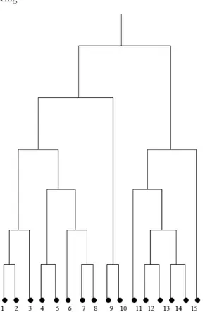
Instead of a single partition of the input dataset, hierarchical clustering approaches output a hierarchy of clustering solutions that are organized into a so-called dendrogram [JD88], i.e., is a tree aimed at graphically describing such a hierarchy (cf. Fig. 2.22_).

Definition 2.2(dendrogram). A dendrogram defined over a set D of data objects is a set T = {T1, . . . , TT} of cluster pairs, where Tt= hTt0, Tt00i, Tt0 ⊆ D, T00

t ⊆ D, ∀t ∈ [1..T ], and: 1.T00

t ⊂ Tt0, ∀t ∈ [1..T ]

(40)

22 2 Clustering

Fig. 2.2. A dendrogram showing a possible cluster hierarchy built upon a simple dataset of 16 data objects

2.T00

t ∩ Tt000 = ∅ and T_t0⊇ T_t00∪ T_t000, ∀t, t0∈ [1..T ] such that t 6= t0 and T_t0 =

T0 t0

Any dendrogram defined according to Def. 2.2 can be alternatively defined by taking into account the levels of the tree. The top level LQ (i.e., the root of the tree) contains a single cluster composed by all the objects in the input dataset, whereas in the bottom level L0 (i.e., the level containing the leaves of the tree) there are singleton clusters, i.e., clusters composed by exactly one input object. Intermediate levels contain partitions of the input dataset at a different granularity. In particular, each level Lq, ∀q ∈ [1..Q−1] comprises a number of clusters lower than that of level Lq−1and greater than that of level Lq+1; this property clearly leads to clusters having average size directly pro-portional to the corresponding level number q. A level-organized dendrogram can be formally defined as follows.

Definition 2.3(level-organized dendrogram). Let T be a dendrogram defined over a set D of data objects. A level-organized dendrogram derived

(41)

2.3 Hierarchical Clustering 23

Algorithm 2.3 standard AHC

Input: a set D = {o1, . . . , on} of data objects;

Output: a level-organized dendrogram T`= [L0, . . . , LQ] defined over D

1: C ← {{o1}, . . . , {on}} 2: L0← C 3: repeat 4: hC0_{, C}00_{i ← closestClusters(C)} 5: C ← C \ {C0_{, C}00_{} ∪ {C}0_{∪ C}00_} 6: append(T`, C) 7: until |C| = 1

from T is a list T`= [L0, . . . , LQ], where each Lq, q ∈ [0..Q], is a partition of D, and:

1.|L0| = |D| 2.|LQ| = 1

3.|Lq| > |Lq+1|, ∀q ∈ [0..Q−1]

Hierarchical clustering algorithms can be classified into two main cate-gories, namely Agglomerative Hierarchical Clustering (AHC) and Divisive Hi-erarchical Clustering (DHC) [JD88]. The difference between these two kinds of approaches lies in the way how the dendrogram is computed. Agglomerative algorithms start from the bottom level of the tree, and build the dendrogram in a bottom-up way. According to divisive approaches the dendrogram is built in a top-down way, by starting from the root of the tree.

The standard AHC scheme follows a greedy approach (cf. Alg. 2.3). Given an input dataset D of size n, the starting point is a partition of D composed by n singleton clusters. Such a partition composes the bottom level of the den-drogram. At each iteration, the current level of the dendrogram is computed by merging the “closest” pair of clusters in the previous level. This strategy clearly leads to a dendrogram whose levels contain a number of clusters equal to that of the previous level minus one. Hence, the algorithm terminates after n − 1 iterations, i.e., when the whole tree has been built.

Linkage Metrics

A crucial point in the standard AHC scheme is the choice of a proper linkage metric, i.e., a criterion to decide which is the closest pair of clusters to be merged at each iteration [Mur83, Mur85, DE84]. Classic linkage metrics comprise single link (SL) [Sib73], complete link (CL) [Def77], average link (AL) [Voo86], and prototype link.

According to SL, CL, and AL metrics, also known as graph linkage met-rics [Ols95], the pair of clusters to be merged is chosen by looking at the minimum, maximum, and average among the pairwise distances between the