Multi-Value Numerical Modeling for Special Di erential Problems

(1)

Universit´

a degli Studi di Salerno

DIPARTIMENTO DI MATEMATICA

Scuola Dottorale in Scienze Matematiche, Fisiche e Naturali Ciclo XIII

Multi-Value Numerical Modeling

for Special Differential Problems

Author:

Giuseppe De Martino

Principal Supervisor:

Prof. Beatrice Paternoster

Associate Supervisor:

Dr. Raffaele D’Ambrosio

PhD Director:

(2)

Introduction

The subject of this thesis is the analysis and development of new numerical methods for Ordinary Differential Equations (ODEs). This studies are motivated by the fundamental role that ODEs play in applied mathematics and applied sciences in general. In particular, as is well known, ODEs are successfully used to describe phenomena evolving in time, but it is often very difficult or even impossible to find a solution in closed form, since a general formula for the exact solution has never been found, apart from special cases. The most important cases in the applications are systems of ODEs, whose exact solution is even harder to find; then the role played by numerical integrators for ODEs is fundamental to many applied scientists. It is probably impossible to count all the scientific papers that made use of numerical integrators during the last century and this is enough to recognize the importance of them in the progress of modern science. Moreover, in modern research, models keep getting more complicated, in order to catch more and more peculiarities of the physical systems they describe, thus it is crucial to keep improving numerical integrator’s efficiency and accuracy.

The first, simpler and most famous numerical integrator was introduced by Euler in 1768 and it is nowadays still used very often in many situations, especially in edu-cational settings because of its immediacy, but also in the practical integration of simple and well-behaved systems of ODEs. Since that time, many mathematicians and applied scientists devoted their time to the research of new and more efficient methods (in terms of accuracy and computational cost). The development of numer-ical integrators followed both the scientific interests and the technolognumer-ical progress of the ages during whom they were developed. In XIX century, when most of the cal-culations were executed by hand or at most with mechanical calculators, Adams and Bashfort introduced the first linear multistep methods (1855) and the first Runge-Kutta methods appeared (1895-1905) due to the early works of Carl Runge and Martin Kutta. Both multistep and Runge-Kutta methods generated an incredible amount of research and of great results, providing a great understanding of them and making them very reliable in the numerical integration of a large number of practical problems.

It was only with the advent of the first electronic computers that the computa-tional cost started to be a less crucial problem and the research efforts started to move towards the development of problem-oriented methods. It is probably possible to say that the first class of problems that needed an ad-hoc numerical treatment was that of stiff problems. These problems require highly stable numerical integrators (see Section 1.7) or, in the worst cases, a reformulation of the problem itself.

Crucial contributions to the theory of numerical integrators for ODEs were given in the XX century by J.C. Butcher, who developed a theory of order for Runge-Kutta

(5)

methods based on rooted trees and introduced the family of General Linear Methods together with K. Burrage, that uniﬁed all the known families of methods for ﬁrst order ODEs under a single formulation. General Linear Methods are multistage-multivalue methods that combine the characteristics of Runge-Kutta and Linear Multistep integrators.

In recent times, the researchers started to develop new methods designed for the efficient solution of particular problems, i.e. taking into account the specific expres-sion and properties of the problem itself and paying attention to the preservation of the intrinsic structures of the solutions in the numerical approximation. This is for example the case of exponentially fitted methods, introduced by L. Gr. Ixaru, which are especially designed for oscillatory or periodic problems. Another import-ant example is that of geometric integrators, that are also one of the main topics of the present thesis. The main idea behind such integration techniques is that of preserving the geometric properties of the solution of an ODE system, such as the presence of invariants or the belonging of the solution to a particular surface. This is for example the case of conservative mechanical systems or of systems with space constraints. It is obvious that the numerical solution of such problems must share these properties of the exact one, or its practical usefulness would be poor and even its significance would be lost. We can think for example to the motion of planets of the Solar System, which move on closed planar trajectories (ellipses): we need a numerical integrator to provide closed trajectories, or the approximation of the motion would be completely useless.

The main result achieved in this thesis is the construction of four nearly-conservative methods belonging to the family of General Linear Methods. In particular, two of these methods proved to be very eﬃcient also compared to classical methods both in terms of computational cost and accuracy. We also studied some theoretical aspects of these techniques, highlighting the presence of parasitic components in the numerical approximation and ﬁnding a condition for their boundedness. Para-sitic components arise in the application of General Linear Methods due to their multivalue nature and they cannot be completely removed, but only controlled, in order to avoid them to destroy the overall accuracy of the numerical scheme. We found an algebraic condition under which the parasitic components give a bounded contribution to the numerical solution and this is small enough to avoid the per-turbation of the geometric properties that we aim to preserve. We also addressed the question of which link exists between the accuracy of a numerical scheme and its ability to preserve geometric invariants, providing a Theorem regarding the family of non-parasitic B-series methods.

Another important class of problems that deserves a special treatment is that of the special second order autonomous ODE presented in Section 2.2. For these prob-lems, R. D’Ambrosio, E. Esposito and B. Paternoster introduced a general family of numerical methods extending the ideas of General Linear Methods. This new family is called the General Linear Nystr¨om (GLN) methods family. The original contribution to this theory that is presented in this thesis is the formulation of an algebraic theory of the order based on a particular set of bi-colored rooted trees. Since GLNs are multivalue methods, an initial approximation of the starting values must be provided by the user. This can be avoided by forging our methods around the so-called Nordsieck vector, i.e. requiring our method to approximate the solution

(6)

and its derivatives, whose initial approximations can be computed exactly from the initial value provided by the problem. We studied in deep this important subclass of numerical integrators, exploiting the expression of the order conditions and proving a theorem where the explicit expression of the local truncation error has been found. The thesis is organized as follows: the first Chapter is devoted to basic defini-tions and properties concerning ODEs and numerical methods. In particular, the well-posedness problem is addressed and a few examples from the applications are presented. We also introduce numerical methods and their basic properties, such as order and stability. The methods presented in this Chapter are the classical Lin-ear Multistep and Runge-Kutta families. Chapter 2 is devoted to General LinLin-ear Methods, both for first and second order differential problems. In this Chapter we introduce the theory of order for General Linear Nyström methods and the other results discussed above. The discussion on geometric integration is performed in Chapter 3, where we present more in detail the geometric properties of ODE sys-tems and of numerical methods and introduce the concept of G-symplecticity, that is the main conservation property we require General Linear Methods to possess. The final Chapter concerns the topics studied by the author in two academic vis-its to the Department of Computer Science of the University of Oxford, namely the extraction on cardiac tissue structure information from a particular Magnetic Resonance Imaging technique.

(7)

(8)

Chapter 1 Ordinary Differential Equations:

Mathematical Background and

Introduction to Numerical

Integration

In this Chapter, we will give the basic definitions and concepts regarding the theory of Ordinary Differential Equations (ODEs). In particular, we recall the general formulation of a system of ODEs, we give a short classification of various types of ODEs and a list of examples. The question of existence and uniqueness of a solution, that is fundamental in Numerical Analysis, is answered by means of the classical Cauchy’s Theorem and some basic stability and geometric properties are listed.

1.1 Introduction

An Ordinary Differential Equation (ODE) (compare [1, 2, 26, 77, 109]) of order n is an equation of the form

F (y(n)(x), y(n−1)(x),· · · , y′(x), y(x), x) = 0, (1.1) where F is deﬁned in a subset of Rn+2 and takes values in R and the unknown function is y : R −→ R. An ODE is said to be in normal form if in (1.1) it is possible to isolate the maximum order derivative, i.e.

y(n)(x) = f (y(n−1)(x),· · · , y′(x), y(x), x), (1.2) with f :Rn+1 −→ R. Notation (1.1) can be extended to systems of ODEs

         F1(y (n) 1 , y (n) 2 ,· · · , y (n) d ,· · · , y1′, y′2,· · · , yd′, y1, y2,· · · , yd, x) = 0 F2(y (n) 1 , y (n) 2 ,· · · , y (n) d ,· · · , y1′, y′2,· · · , yd′, y1, y2,· · · , yd, x) = 0 .. . Fd(y(n)1 , y (n) 2 ,· · · , y (n) d ,· · · , y1′, y2′,· · · , yd′, y1, y2,· · · , yd, x) = 0,

(9)

A ﬁrst result concerning systems of ODEs is that an equation of order n can always be written as a system of n ﬁrst order equations. In fact, if we consider an order n equation (in normal form, to simplify the notations)

y(n)(x) = f (y(n−1)(x),· · · , y′(x), y(x), x), deﬁning _         z1 = y z2 = y′ .. . zn= y(n−1),

we obtain the ﬁrst order system              z₁′ = z2 z₂′ = z3 .. . z_n′₋₁ = zn z_n′ = f (zn, zn−1,· · · , z1, x).

Note that this procedure can be applied recursively to systems of d equations of order n, thus obtaining a system of nd ﬁrst order equations. It is then convenient and exhaustive to introduce the following vector notation

y′ = f (x, y) (1.3)

with y :R −→ Rdand f :Rd+1−→ Rd. A solution of (1.3) is a function ¯y :R −→ Rd

such that ¯y′ = f (x, ¯y).

Depending on the properties of the function f , equation (1.3) can be further classiﬁed, e.g. if f is linear with respect to y, the equation is said to be linear, if f do not depend explicitly on x, then the equation is called autonomous.

Example 1.1.1. The forced Van Der Pol oscillator [64] describes an electrical or

mechanical oscillator with non-linear attenuation {

y₁′ = y2

y₂′ = b(1− y2

1)y2− ω2y1+ a cos(Ω∗ x)

and is an example of ﬁrst order system of two equations depending on four para-meters a, b, ω, Ω.

We observe that a system (1.3) can always be written in the autonomous form, just rewriting the unknown vector function y as a d + 1-sized vector, being the new component the identity function of x, i.e.

             y′₁ = f1(yd+1, y1, y2,· · · , yd) y′₂ = f2(yd+1, y1, y2,· · · , yd) .. . y′_d = fd(yd+1, y1, y2,· · · , yd) y′_d+1 = 1.

(10)

1.1.1 The Initial Value Problem

As observed in the Introduction, ODEs are a fundamental tool to model phenomena evolving in time. In many practical applications, ODEs are given together with an

initial condition, describing the status of the system at a certain point in time. We

deﬁne then an Initial Value Problem (IVP) as a system of ODEs coupled with an initial condition, i.e. _{

y′ = f (x, y)

y(x0) = y0.

(1.4) A solution of (1.4) is a solution ¯y of the ODE such that ¯y(x0) = y0. For the numerical

treatment that will follow in next Sections, it is fundamental to understand when an IVP is a Hadamard well-posed problem, i.e. when

• there exist a solution; • the solution is unique;

• the solution has a continuous dependency on the data.

In order to recall some results concerning well-posedness, we need the deﬁnition of Lipschitz-continuous function.

Definition 1.1.1. A function f : [a, b]× Rd −→ Rd is Lipschitz-continuous with

respect to the second argument if there exist a real number L, called Lipschitz

constant, such that

∥f(x, y1)− f(x, y2)∥ ≤ L∥y1− y2∥ (1.5)

for each x∈ [a, b].

The ﬁrst two points of well-posedness are answered by the classical [1, 2, 11, 26, 77, 109]

Theorem 1.1.1 (Cauchy’s Existence and Uniqueness). Given an IVP

{

y′ = f (x, y)

y(x0) = y0

if f is continuous in an open neighborhood of the initial condition (x0, y0), uniformly

with respect to x and Lipschitz-continuous with respect to y, then there exist an unique solution of the given IVP.

Under the same hypotheses it can be proved that the solution depends continu-ously on the data, that is the third condition to be satisﬁed in order to have a well posed problem.

Theorem 1.1.2. Given an IVP

{

y′ = f (x, y)

y(x0) = y0

, x∈ [x0, X], (1.6)

consider the perturbed problem {

y′ = ˜f (x, y) y(x0) = ˜y0

(11)

being f, ˜f deﬁned and continuous in [x0, X]× Rd.

Let y and ˜y be solutions respectively of (1.6)and of of (1.7). If there exists an ϵ∈ R such that

∥f(x, η) − ˜f (x, η)∥ ≤ ϵ

for each x∈ [x0, X] and for each η∈ Rdand f is Lipschitz-continuous with Lipschitz

constant L, then

∥y(x) − ˜y(x)∥ ≤ ∥y0− ˜y0∥eL(x−x0)+

ϵ L(e

L(x−x0)− 1),

thus providing an upper bound for the normed diﬀerence between the solutions of the given problems.

1.2 Examples

ODEs arise naturally as models in a large number of applied sciences. In this Section some examples are collected and analysed.

1.2.1 Models from Life Sciences

Example 1.2.1 (Population Growth). Population growth models apply to a

num-ber of areas of applied and social sciences, such as Biology, Chemistry, Demography, Economics, Immunology and Physics. Aiming to introduce a basic model, we con-sider an isolated population, i.e. a population such that the only causes of variation in the number of elements are birth and death. The Malthusian Model [41] describ-ing the growth of such a population is the followdescrib-ing ODE

N′(t) = (λ− µ)N(t) (1.8)

where N (t) is the number of elements at time t and λ, µ are respectively the birth and death rates. If we ﬁx an initial condition N (0) = N0, the solution of (1.8) is an

exponential

N (t) = N0exp

λ µt.

Malthusian model provides an indeﬁnitely growing solution for the number of indi-viduals in a population, then it is not realistic for long time-spans. An improvement can be introduced using the so called carrying capacity parameter K, i.e. a para-meter controlling the growth of the solution and related to the environment where the population is set. Such a modiﬁcation leads to the logistic model [41]

N′(t) = λ µN (t) ( 1− N K )

whose solution grows up to a certain level of saturation and then remains stable asymptotically. More recent models take into account a larger number of factors and are very specialized for each ﬁeld of application. One can think for example to a time-varying carrying capacity, to models embedding catastrophes or multiple population, or to stochastic models [41].

(12)

Next examples are taken from Immunology[116] [76].

Let v be the number of free viruses infecting a body and let x and y be the number of uninfected and infected cells respectively. Uninfected cells are produced at a rate λ and die at a rate d. Such new born cells are susceptible of infection if they meet a virus and become infected with rate β. Infected cells die at a rate a. The viruses population elements die at a rate u but each infected cell produces a number of new viruses; let k be the rate of birth of the viruses in an infected cell. Combining those information, we get to the following three-populations model [116]

   x′ = λ− dx − βxv y′ = βxv− ay v′ = ky− uv.

Example 1.2.2. We present a recent model describing an infection of inﬂuenza A

virus. Its mathematical expression presents an embedding of ODEs and PDEs. We denote respectively with T and I the number of uninfected and infected target cells and with Ta and Ia their apoptotic1 counterparts.

           dT dt = µT − r Inf_T _{− K}Apo T T, ∂I ∂t + ∂I ∂τ =− ( k_TApo+ k_tApo(τ ) ) I(t, τ ), dTa dt = h Apo T T − rinfTa− kLysTa, dIa dT = ∫_∞ 0 ( kApo_T − k_IApo(τ ) ) I(t, τ )dτ + rInf_T a− kLysIa, where µ = [ µmax Tmax ( Tmax− T − ∫ _∞ 0 I(t, τ )dτ )] + .

Here µ is the speciﬁc growth rate of uninfected cells and kApo_T their apoptosys rate (analogous notation is used for infected cells). The parameters rInf, Tmax and µmax

are respectively the infection rate, the maximum concentration of cells and the maximum speciﬁc rate.

We observe that this model follows two time scales, the absolute time t and the cells age τ .

Example 1.2.3. The FitzHugh-Nagumo model [112, 61]

{_dv

dt = c1v(v− a)(1 − v) − c2w + iapp dw

dt = b(v− c3w)

(1.9) contains an example of cubic equation. The variable v describes the transmembrane potential in a living cell, while w is called recovery variable and was introduced to improve the original model. The parameters a, b, c1, c2, c3 can be adjusted to

simulate diﬀerent types of cell.

1.2.2 Models from Physics

Newton’s second law, connecting the force applied on a material point of mass m with the acceleration it receives in an inertial system [70, 75], is a second order ODE

F = ma. (1.10)

(13)

Example 1.2.4. In a more rigorous fashion, let y(t) be the position of the material

point at time t in R3_{, equation (1.10) takes the form}

y′′(t) = F (t, y, y′).

Some particular classical examples are the harmonic oscillator

y′′ =−ω2y,

and the motion of a body under the gravity force into the void

y′′ =−g.

Example 1.2.5. Another example of a second order ODE in Physics, in particular

in the ﬁeld of electromagnetism [75], is

LI′′+ RI′+ C−1I = f (t)

describing the current I(t) in an LRC circuit with applied power f (t).

Example 1.2.6. The radial Schr¨odinger equation

y′′+ (E− V (x))y = 0 (1.11) is a fundamental equation of quantum physics describing the behaviour of a particle in a spherically symmetric potential V (x). E is the energy associated to the system and the interest in this equation is generally twofold

• in its IVP formulation, it provides the trajectory followed by the particle; • in its formulation as a boundary value problem it provides the admissible

values of the energy E, that are the eigenvalues.

1.2.3

1.3 Hamiltonian Systems

Hamiltonian systems are a class of ODEs mainly used in modeling mechanical sys-tems. This Section is devoted to the description of the basic properties of such systems. Some examples are shown.

1.3.1 History and Motivations

Mechanics is the branch of Physics studying the motion of bodies by means of Differential Equations. The first equations of mechanics appeared in Galilei’s and Newton’s works, in particular the former introduced the celebrated equation (1.10). In 1788, Lagrange introduced his Analytical Mechanics, making the analysis of mech-anical systems easier also in complex cases. The main simplification introduced by Lagrange was the adoption of generalized coordinates (q1, q2,· · · , qd) to describe the

state of a system with d degrees of freedom. For example, a material point that is bonded to move on a surface will have two degrees of freedom, so its motion can be described using only two variables instead of the three required in Newtonian Mechanics. Let T = T (q, ˙q) be the kinetic energy of a system with d degrees of

freedom and U = U (q) its potential energy, we deﬁne the Lagrangian function of the system as the diﬀerence

L = T − U.

2_{i.e. the energy per unit volume of water required to transfer an infinitesimal quantity of water}

(15)

At each time point, the generalized coordinates of the system satisfy the so-called

Lagrange’s equations of motion d dt( ∂L ∂ ˙q) = ∂L ∂q

providing a system of d second order ODEs. W.R. Hamilton introduced a further simpliﬁcation adopting the so-called conjugate momenta

pk=

∂L

∂ ˙q(q, ˙q) k = 1,· · · , d (1.12)

in place of the generalized velocities ˙q. The Lagrangian function can be rewritten

as the so-called Hamiltonian function

H(p, q) := pT

˙

q− L(q, ˙q),

where ˙q can be expressed in terms of p and q by means of equation(1.12). Hamilton’s equations of motion [34, 57, 59, 63, 66, 97] are given by

   ˙ pk=−_∂q∂H k ˙ qk= _∂p∂H_k k = 1,· · · , d (1.13)

providing a system of 2d ﬁrst order ODEs .

1.3.2 Examples

We provide a few examples of Hamiltonian systems. Other and more complex ex-amples are given in Section 3.1

Example 1.3.1 (Harmonic Oscillator). A simple harmonic oscillator is a system

made by a material point (we assume here of unitary mass) linked to a spring. The equations of motion are _{

p′ =−q

q′ = p with the Hamiltonian

H = p2

2 +

q2

2.

Example 1.3.2 (Simple Pendulum). A simple pendulum is a mechanical system

made by an unitary mass connected to an inextensible rope of negligible mass. If we assume the gravity force to be unitary, the equations of motion are

{

p′ =− sin q

q′ = p and the Hamiltonian function is

H = p2

(16)

Example 1.3.3 (Kepler’s Problem). The following Hamiltonian system describes

the motion of a planet around the origin, where a ﬁxed sun is supposed to lie          q₁′ = p1 q₂′ = p2 p′₁ = −q1 (q2 1+q22) 3 2 p′₂ = −q2 (q2 1+q22) 3 2.

The Hamiltonian function has the form

H = 1 2(p 2 1+ p 2 2)− 1 √ q2 1 + q22 .

1.3.3 Geometric properties of Hamiltonian systems

Hamiltonian systems are widely studied in the field of geometric numerical integ-ration, since they own two important conservation properties: energy conservation and the symplecticity of the flow [59, 70]. Concerning the preservation of the total energy, we observe that the Hamiltonian function of each Hamiltonian system is a first integral of the system itself. This can be verified immediately just deriving H with respect to the time variable

dH dt = ∑ i ∂H ∂pi dpi dt + ∂H ∂qi dqi dt (1.14)

evaluating (1.14) in a solution of the system we obtain

dH dt = ∑ i dqi dt dpi dt − dpi dt dqi dt = 0.

We are not going into the mathematical details of symplecticity of the ﬂow, since such a treatment would require advanced mathematical tools that are beyond the purposes of this work (for more details, see [70]).

We will give here a geometric idea of what symplecticity of the flow of an Hamilto-nian system means. We first recall the definition of flow of a dynamical system as the operator

Ψ (p(0), q(0)) 7→ (p(t), q(t)) .

Such an operator is said to be symplectic if it preserves volumes. In particular, in the case of a system with one degree of freedom, that will provide a two dimensional domain for Ψ, the ﬂow is symplectic if it preserves oriented areas.

1.3.4 Quadratic Invariants

Consider an homogeneous ODE

y′ = f (y). (1.15)

A quadratic function

I(y) = yTQy (1.16) where Q is a symmetric matrix is an invariant for (1.15) if, and only if

(17)

Example 1.3.4 (Inertial motion of a rigid body). Euler’s equations for the inertial

motion of a rigid body are _     ˙ ωx = ( Iyy−Izz Ixx )ωyωz ˙ ωy = (Izz_I−I_yyxx)ωzωx ˙ ωz = (Ixx_I−I_zzyy)ωxωy

where ωx, ωy, ωz are the components of the angular speed along the principal axes

of inertia and Ixx, Iyy, Izz are the principal inertia momenta. This system possesses

two quadratic invariants, namely the kinetic energy K and the square norm of the angular momentum A, i.e.

K = 1 2 [ ωx ωy ωz ]_ Ixx 0 0 0 Iyy 0 0 0 Izz     ωωxy ωz   , A =[ ωx ωy ωz ]_ Ixx2 0 0 0 I_yy2 0 0 0 I_zz2     ωωxy ωz   .

1.4 Introduction to Numerical Integration

The numerical integration of an IVP by means of classical integrators usually in-volves working on a discretized version of the IVP itself, thus introducing an intrinsic error, that is called Local Truncation Error (LTE). A numerical method is said to be consistent if LTE tends to zero with the integration step going to zero.

1.4.1 Finite Differences

Before going into the details of numerical integrators, it is appropriate to recall a classical method for the approximation of derivatives: ﬁnite diﬀerences.

By deﬁnition, the ﬁrst derivative of a function f in a point x is given by the limit

f′(x) = lim

h→0

f (x + h)− f(x) h

if it exists. Neglecting the limit operator and taking a ﬁxed value for h we obtain an approximation of f′(x)

f′(x) = f (x + h)− f(x)

h + O(h)

involving the so-called first order forward difference [4, 106, 108] ∆h[f ](x) =

f (x + h)− f(x)

h . (1.17)

Another ﬁrst order approximation of f′(x) can be obtained using the first order

backward difference

∇h[f ](x) =

f (x)− f(x − h)

(18)

while the central difference

δh[f ](x) =

f (x + 1₂h)− f(x − 1₂h) h

provides a second order approximation.

Hihger order finite differences, useful to approximate higher order derivatives, can be obtained by means of recursive application of the first order ones. An example that is widely used is the second order central difference

δ2_h[f ](x) = f (x + h)− 2f(x) + f(x − h)

h2

providing an approximation of f′′(x).

1.4.2 The Euler’s method

We consider an IVP _{

y′ = f (x, y)

y(x0) = y0

, x∈ [x0, X] (1.18)

and approximate the first derivative just with a first order difference (1.17). The differential equation in (1.18) becomes

y(x0 + h)− y(x0) = hf (x0, y(x0)) + O(h).

Neglecting the O(h) term, we get one step of the Euler’s method.

y(x0+ h)≈ y(x0) + hf (x0, y(x0)) (1.19)

and iterating on a ﬁxed stepsize discretization of [x0, X]:

∆ ={x0+ nh, n = 0, 1,· · · , N} ,

we obtain the following approximation of the solution

yn+1 = yn+ hf (xn, yn), n = 0, 1,· · · , N − 1. (1.20)

The numerical approximation of (1.18) is no more a diﬀerential equation, but a

dis-cretized version of it. Classical numerical integrators do not deal with the continuous

problem, but with a discretization of it, usually by means of a diﬀerence equation. New problems then arise at this step: is the discretized problem well-posed? Is it a good approximation to the original problem?

1.4.3 Difference Equations

A difference equation [56] is a recurrence relation, i.e. a relation involving the values of a function in a discrete number of points, formally

F (yn, yn+1,· · · , yn+k) = 0, (1.21)

where k is the order of the equation. We are interested in ﬁnding a solution of (1.21), that is a sequence of values that makes (1.21) an identity. Deﬁnitions of

(19)

linearity, homogeneity and expression in normal form can be given and are analogous to those given for ODEs.

Many numerical methods produce linear diﬀerence equation with constant coef-ﬁcients, namely of the form

αkyn+k+ αk−1yn+k−1+· · · + α0yn= gn, (1.22)

being gn the forcing term.

Example 1.4.1. The equation

yn+1− yn= n− 2

is ﬁrst-order, linear and constant coeﬃcients with forcing term gn = n− 2. Given

the initial value of the solution, we can obtain the whole sequence just applying recursively the equation. Another example is the Euler’s method formula (1.20).

Well-posedness of diﬀerence equations is crucial in the analysis of numerical integrators. The following theorem is the analogous of Theorem 1.1.1 for equations like (1.22)

Theorem 1.4.1. The linear diﬀerence equation of order k with constant coeﬃcients

αkyn+k + αk−1yn+k−1+· · · + α0yn = gn

has a unique solution for each k-uple of initial values.

The following result gives much insight in what can happen to the solutions of (1.22)

Theorem 1.4.2. Consider the equation (1.22),

1. if gn= 0 and y0 = y1 =· · · = yk−1 = 0, then the only solution is a sequence of

zeros;

2. if{yn} and {zn} are solutions, then {Ayn+Bzn} is a solution for each A, B ∈ R;

A system of k linearly independent solutions3 _{of (1.22) is said fundamental} system of solutions. We now consider the homogeneous equation

αkyn+k + αk−1yn+k−1+· · · + α0yn= 0 (1.23)

and search for its solutions of the form {yn} = {zn}, z ̸= 0. Substituting in (1.23),

we obtain

αkzn+k + αk−1zn+k−1+· · · + α0zn = 0

that is equivalent to

αkzk+ αk−1zk−1+· · · + α0 = 0. (1.24)

The polynomial at ﬁrst member in (1.24) is called characteristic polynomial of eqre-ﬂinom and{zn} is a solution of (1.23) if and only if z is a root of the characteristic polynomial, moreover, the following result holds

3_{The sequences}_{y

n} and {zn} are said to be linearly independent in n = n0if and only if the

(20)

Theorem 1.4.3. Let z1, z2,· · · , zk be the roots of the characteristic polynomial of

equation (1.23), then

• if zi ̸= zj for each i̸= j, then {{zn1}, {z2n}, · · · , {zkn}} is a fundamental system

of solutions for (1.23);

• if zi is a multiple root of order l > 1, then {zin}, {nzin}, · · · , {nl−1zni} are

solutions and a fundamental system of solutions can be obtained just joining this set of solutions with those related to the other roots.

In view of some observations concerning stability, it is important to analyze the behavior of the solutions of a diﬀerence equation, in particular we distinguish tree cases

1. z is a simple real root, then {zn} is a solution of (1.23) it diverges if |z| > 1,

while it goes to zero if|z| < 1 and is bounded if |z| = 1;

2. z is a complex root, then its conjugate ¯z is a root. If z = α+iβ, the

correspond-ing solutions are {zn} = {(α + iβ)n} and {¯zn} = {(α − iβ)n}, corresponding, if z = ρ(cos θ + i sin θ), to the trigonometric form

{ρn_{sin nθ}_{} , {ρ}n_{cos nθ}_},

thus oscillating in [−ρ, ρ];

3. z is a multiple root of order l: we obtain l solutions{zn}, {nzn}, . . . , {nl−1zn},

diverging if |z| ≥ 1 and going to zero if |z| < 1.

In numerical integration we obviously want our approximation to be bounded, so we only consider as good those methods whose associated difference equation has a characteristic polynomial with roots of modulus less or equal then one but being the roots of modulus one simple. This is a first “raw“ definition of stability. Method (1.20) is a linear first-order difference equation, whose characteristic polynomial is

z− 1.

1.5 Linear Multistep Methods

Consider an IVP {

y′ = f (x, y)

y(x0) = y0.

, x∈ [x0, X] (1.25)

and a discretization{xi} of the interval [x0, X]. The general expression of a k-step

Linear Multistep Method (LMM) [11, 71, 86] is

k ∑ j=0 αjyn+j = h k ∑ j=0 βjf (tn+j, yn+j). (1.26)

Example 1.5.1. Integrating the ODE in (1.25) in a subinterval of the discretization

[xi, xi+1] we obtain

y(xi+1)− y(xi) =

∫ xi

xi+1

f (τ, y)dτ . (1.27) Approximating the integral in (1.27) with diﬀerent quadrature formulas gives rise to diﬀerent LMM, e.g.

(21)

• using a trapezoidal formula and neglecting the associated error we obtain yi+1− yi =

h

2(f (xi+1, yi+1) + f (xi, yi)) , called again trapezoidal rule;

• using as approximation the surface of a rectangle based in xi, xi+2and of height

f (xi+1 we obtain the mid-point rule

yi+2− yi = 2hf (ti+1, yi+1).

These two examples are useful to the purpose of introducing the issues that are generally related to the application of LMM, in fact the mid-point rule is a two step method, needing a starting value that is generally not provided by the problem. Such a starting value is often obtained applying a one step method or using other strategies. In trapezoidal rule the unknown value yi+1 appears as a variable of the

function f , giving rise to a generally non linear equation.

Definition 1.5.1. A LMM (1.26) is called explicit if αk = 0, otherwise it is called

implicit.

Remark 1.5.1. Implicit methods involve the solution of a non linear equation or

system of equations, that is generally effectively solved using fixed-point iterations. In equation (1.26) it is possible to rescale the coefficients in such a way that αk= 1.

If we assume the method to be implicit, we can write

yn+k =− k−1 ∑ j=0 αjyn+j + h k ∑ j=0 βjf (xn+j, yn+j). (1.28)

This can be viewed as a ﬁxed point iteration x = g(x) and it can be numerically solved by means of an iterative procedure

x(k+1) = g(x(k))

which is convergent e.g. if g is a contraction4. In equation (1.28), if we collect in A the terms independent from yn+k we have the following expression for g

g(y) = A + hβkf (xn+k, y).

We want this function to be a contraction

|g(y1)− g(y2)| = |hβk(f (xn+k, y1)− f(xn+k, y2))| ≤ |hβkL||y1− y2|

where L is the Lipschitz constant of the function f . The ﬁxed point iteration is then convergent if h < 1

|βk|L.

(22)

1.5.1 Consistency and Order Conditions of LMM

Associated to a LMM k ∑ j=0 αjyn+j = h k ∑ j=0 βjf (xn+j, yn+j), is a diﬀerence operator [86] L [y(x); h] = k ∑ j=0 αjy(x + jh)− hβy′(x + jh). (1.29)

The operator L, if evaluated in the solution y of an IVP, returns the residual of the solution itself in the method, i.e. the LTE. We are interested in ﬁnding conditions on the coeﬃcients of the method for LTE being of a certain order. To do that, we write the Taylor’s expansion of L in a neighborhood of x

L [y(x); h] = k ∑ j=0 αj [ y(x) + jhy′(x) + j 2_h2 2 y ′′_{(x) + . . . +} jqhq q! y (q)_{(x) + . . .} ] − − h k ∑ j=0 βj [ y′(x) + jhy′′(x) + j 2_h2 2 y ′′′_{(x) + . . . +}jqhq q! y (q+1)_{(x) + . . .} ]

and collect the coeﬃcients of the derivatives of y

c0 = k ∑ j=0 (αj) c1 = k ∑ j=0 (jαj− βj) c2 = k ∑ j=0 (j2αj 2 − jβj) .. . cq = k ∑ j=0 (jqαj q! − jq−1βj (q−1)!) (1.30)

Definition 1.5.2. A LMM has order p if its coeﬃcients ci deﬁned in (1.30), are

zero for each i less then or equal to p and cp+1 is not zero.

cp+1 is called main term of LTE.

Definition 1.5.3. A LMM is consistent if its order is at least one.

1.5.2 Zero-stability and Convergence

Zero-stability of a LMM is related to the stability of the underlying diﬀerence oper-ator [11, 86].

(23)

Definition 1.5.4. We consider a LMM (1.26). The polynomials ρ(z) = k ∑ j=0 αjzj and σ(z) = k ∑ j=0 βjzj

are respectively called first and second characteristic polynomial of the method. Applying the results shown in Section (1.4.3) we can give the following

Definition 1.5.5. A LMM is zero–stable if the roots of its ﬁrst characteristic

poly-nomial are all less or equal to one in modulus and those whose modulus is equal to one are simple.

Convergence, as we will see more in detail in next sections, is the property of a method ensuring the numerical approximation to tend to the exact solution as the stepsize goes to zero. In order to give a suitable definition of convergence for LMM, we need to take into account the necessity of starting values that may affect the overall integration process. Following [86], we define convergence of LMM as follows

Definition 1.5.6. Consider an IVP and let y be its solution and yn(h) the numerical

approximation provided by a k-step LMM method (1.26) with stepsize h. The LMM is convergent if

lim

h→ 0, n → +∞ nh = x− x0

yn(h) = y(x)

for each k-uple of starting values

yµ= ηµ(h), µ = 0, . . . , k− 1

such that

lim

h→0ηµ(h) = y0. (1.31)

Condition (1.31) ensures that the starting values are close enough to the only exact value of the solution that is given us, i.e. the initial value.

Deﬁnition 1.5.6 can be hard to verify. In practical construction processes, the following equivalence is very useful.

Theorem 1.5.1. A Linear Multistep Method is convergent if and only if it is

zero-stable and consistent.

1.6 Runge-Kutta Methods

Runge-Kutta methods (RK) [11, 71, 86] are single-step multi-stage methods. Their complexity relies on a higher number of function evaluation per step, making the

(24)

maximum proﬁt out of the given initial value. A Runge-Kutta method is deﬁned by the following procedure

       Ki = f (tn+ cih, yn+ h s ∑ j=1 aijKj), i = 1, . . . , s yn+1 = yn+ h s ∑ i=1 biKi, (1.32) or, equivalently        Yi = yn+ h s ∑ j=1 aijf (tn+ cjh, Yj), i = 1, . . . , s yn+1 = yn+ h s ∑ i=1 bif (tn+ cih, Yi).

Each step of the computation is further divided into two phases

1. solving the nonlinear system in the ﬁrst equation of (1.32) in order to compute the values Ki, called inner stages of the method;

2. computing the approximation yn+1 using the second equation in (1.32).

Remark 1.6.1. The computation of the stages is the most computationally

ex-pensive task of each step, requiring the numerical solution of a nonlinear system. The dimension of this system, usually denoted with s is the number of stages of the method. A fixed point iteration procedure can be used in order to solve the system, being it in a fixed point form already. In some cases, however, fixed point iterations do not converge and Newton’s method can be used effectively.

RK methods are usually denoted with a tableaux

c1 a11 a12 . . . a1s c2 a21 a22 . . . a2s .. . ... . .. ... cs as1 as2 . . . ass b1 b2 . . . bs,

called Butcher’s tableaux or Butcher’s array [11, 71, 86]; using a matrix notation

A = (aij), c = (c1, . . . , cs), b = (b1, . . . , bs), it becomes

c A

bT .

Coeﬃcients bi are called weights of the method and ci are called abscissae or nodes.

A Runge-Kutta method is said explicit if its coeﬃcient matrix A is strictly lower triangular, otherwise we say that the method is implicit. Explicit methods require a lower computational eﬀort in the computation of the stages, since one can solve the non-linear equations in (1.32) sequentially.

(25)

Example 1.6.1. We can write the Euler’s method and the mid-point rule as RK methods respectively as 0 1 , 0 1 1 1 2 1 2 .

The following methods have order 3 and 4 respectively [11]

0 1 2 1 2 1 −1 2 1 6 2 3 1 6 , 0 1 2 1 2 1 2 0 1 2 1 0 0 1 1 6 1 3 1 3 1 6

Radau II method (order 3, 2 stages) has the tableaux [11]

1 3 1 3 0 1 1 0 3 4 1 4 .

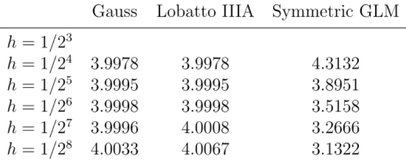
The following methods are based on Gaussian nodes and have respectively order 4 and 6. Gauss methods achieve the maximal order with a ﬁxed number of stages, i.e. 2s if s is the number of stages[11, 71, 70].

3−√3 6 1 4 1 4 − √ 3 6 3+√3 6 1 4 + √ 3 6 1 4 1 2 1 2 (1.33) 1 2 − √ 15 10 5 36 2 9 − √ 15 15 5 36− √ 15 30 1 2 5 36 + √ 15 24 2 9 5 36− √ 15 24 1 2 + √ 15 10 5 36 + √ 15 30 2 9 + √ 15 15 5 36 5 18 4 9 5 18

(26)

1.6.1 Order Conditions

The theory we present in this Section was developed by Butcher, who found a link between the order of a RK method and the elements of the set of rooted trees (see [11]). This theory simpliﬁed a lot the study and construction of RK methods and nowadays it is still actual and still many papers and new theories are based on it. Starting from the ideas of this theory we developed an algebraic theory of order for General Linear Nystr¨om methods for second order ODEs in Section 2.2.1. Many relevant and fundamental contributions have also been given by Hairer and his co-authors (see for example [71, 70]) and by Chartier, Faou and Murua [23].

For the remainder of this Section, in order to simplify the notations, it will be convenient to consider only autonomous initial value problems

y′(x) = f (y(x)), y(x0) = y0.

Butcher’s order theory is based on the observation that a biunivocal correspondence can be found between the derivatives of such problem and the elements of the set of rooted trees we will introduce later in this Section. In practice, the order conditions will be found by comparison between the Taylor expansions of the exact solution and the numerical one. In order to exploit this properties, we write the derivatives of y up to order 3

y′(x) = f (y(x)) (1.34)

y′′(x) = f′(y(x))y′(x) (1.35)

= f′(y(x))f (y(x))) (1.36)

y′′′(x) = f′′(y(x))(f (y(x)), y′(x)) + f′(y(x))f′(y(x))y′(x) (1.37) =f′′(y(x))(f (y(x)), f (y(x)))+f′(y(x))f′(y(x))f (y(x)). (1.38) Note that we used the fact that y is a solution of the diﬀerential problem, thus

y′ = f (y) and we need to compute those derivatives essentially by means of Leibnitz’s rule. Following Butcher (see [11]), we simplify the notations writing f = f (y(x)),

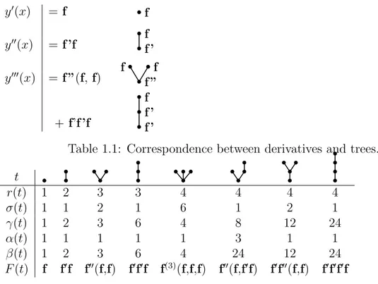
f′ = f′(y(x)), f′′ = f′′(y(x)), . . . , then we observe that these derivatives can be put in correspondence with rooted trees following a simple set of rules

1. a derivative of order n corresponds to a tree with n nodes; 2. each occurrence of f becomes a vertex;

3. a ﬁrst derivative f′ becomes a vertex with one branch;

4. a k-th derivative f(_{k) becomes a vertex with k branches pointing upwards.}

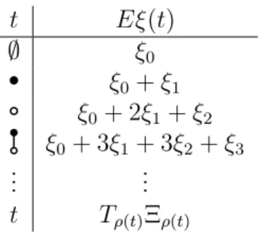
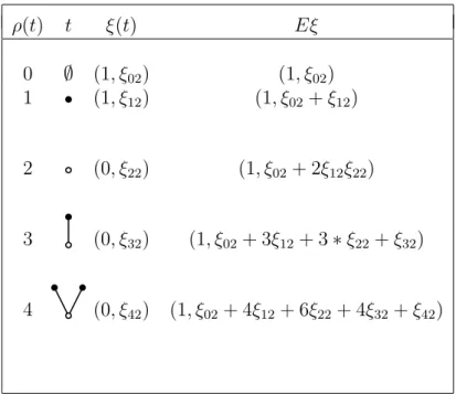
We then obtain Table 1.1 It is now time to introduce a few operators on the set of rooted trees

T ={ , , , , . . .} ,

namely, for a generic tree t∈ T ,

• r(t) is the order of t, i.e. the number of vertices

• σ(t) is the symmetry of t, i.e. the order of the automorphism group of the set

(27)

y′(x) = f f

y′′(x) = f ’f _{f ’}f

y′′′(x) = f ”(f, f) f _{f ”}f + f’f ’f _{f ’}f ’

f

Table 1.1: Correspondence between derivatives and trees.

t r(t) 1 2 3 3 4 4 4 4 σ(t) 1 1 2 1 6 1 2 1 γ(t) 1 2 3 6 4 8 12 24 α(t) 1 1 1 1 1 3 1 1 β(t) 1 2 3 6 4 24 12 24 F (t) f f′f f′′(f,f) f′f′f f(3)(f,f,f) f′′(f,f′f) f′f′′(f,f) f′f′f′f

Table 1.2: Operators on trees up to order 4.

• γ(t) is the density of t

• α(t) is the number of ways of labelling with an ordered set • β(t) is the number of ways of labelling with an unordered set • F (t)(y0) are the elementary diﬀerentials.

Elementary differentials are in practice the various differential terms which combin-ation give the derivatives of y (for more rigorous definitions, see [11, 71]).It is now easy to verify that the exact solution of the given problem y can be expanded in Taylor series around x0 as follows

y(x0+ h) = y0+ ∑ t∈T α(t)hr(t) r(t)! F (t)(y0) (1.39) or, equivalently y(x0+ h) = y0+ ∑ t∈T hr(t) σ(t)γ(t)F (t)(y0)

Next step is to write the numerical approximation provided by a RK method as a series of the form (1.39) and compare the corresponding terms between those two series. We consider expression (1.32) of a Runge-Kutta method and, following [70], we put gi = hki and write

gi = hf (ui), ui = yn+ ∑ j aijgj, yn+1 = yn+ ∑ i bigi. (1.40)

(28)

Now we need to derive these expressions as functions of the stepsize h and evaluate the derivatives in h = 0, since we are interested in the value in yn. Applying

Leibnitz’s rule, we obtain

g_i(q) = h(f(q)(ui)) + q(f(q−1)(ui))

then, in h = 0,

g(_iq) = q(f(q−1)(ui)).

In practice we have the same expression of the derivative of the exact solution multiplied by a term q. This allows us to compute the gi’s derivatives using (1.34),

but we ﬁnd them to depend on the derivative of the ui terms. These terms are easily

computed by linearity, due to the deﬁnition of ui (1.40). It is now easy to combine

all the terms and get the coeﬃcients of the expansion of the numerical solution, that are called elementary weights

Φ(t) =

s

∑

i,j,k=1

biaijc2jaikc2k.

The formal series expansion for the numerical solution is then

y1 = y0 +

∑

t∈T

hr(t)

σ(t)Φ(t)F (t)(y0)

and the order conditions are easily obtained by comparison with (1.39), obtaining the following

Theorem 1.6.1. The Runge-Kutta method (1.32) has order p if and only if

Φ(t) = 1

γ(t)

for each tree t∈ T such that ρ(t) ≤ p.

As anticipated in the introduction to this Section, we found a result analogous to Theorem 1.6.1 for methods belonging to the family of General Linear Nystr¨om methods for second order problems and it is Proposition 2.2.1.

1.7 Linear Stability of Numerical Integrators

Stability is a fundamental property of numerical methods. A method is stable if it is able to handle small errors without amplifying them. Small errors always occur in numerical procedures, due basically to the representation of machine numbers. Other errors are introduced by the numerical procedure, e.g. the LTE (see Section 1.4) in numerical integrators. A stable method is able to keep those perturbations under control in order to avoid them to aﬀect the overall accuracy.

(29)

1.7.1 Introduction

In the numerical integration of initial value problems, stability is classically invest-igated in the linear sense.

Consider an IVP (1.4) and let y and z be solutions respectively corresponding to the initial values y0 and z0; let δy := z− y be the diﬀerence between the solutions. We

aim to ﬁnd a relation connecting the initial values with the corresponding solutions. We derive z using the deﬁnition of δ

z′ = y′+ (δy)′ = f (x, z) = f (x, y + δy), (1.41) and write the Taylor series expansion of f (x, y + δy) based in (x, y), then substitute in (1.41)

y′+ (δy)′ = f (x, y) +∂f

∂yδy + o(||δy||

2_).

Truncating and using the deﬁnition of y we obtain

(δy)′ = J δy + o(||δy||2), (1.42) being J = ∂f_∂y the Jacobian of f .

For linear systems with constant coeﬃcients [86]

y′ = Ay

good stability properties are achieved when the real part of the eigenvalues of A are negative, since in such a case the corresponding solutions are decreasing. We found that the difference δ between two solutions of an IVP satisfies (1.42), i.e. a linear system with non-constant coefficients. It is useful anyway to consider as a test equation

y′ = λy, λ ∈ C (1.43)

or its vector homologous

y′ = Λy

since this allows us to take advantage of the connection between stability and the eigenvalues of Λ. This corresponds to assuming the Jacobian of f to be locally constant, but this is not always coherent with the actual problem.

Example 1.7.1. Consider the system y′ = A(x)y, with

A = [ 0 1 − 1 16x2 − 1 2x ] , x > 0.

A has the only eigenvalue: λ = −_4x1 . If x > 0, λ is negative, so we expect the solutions of the system to be decreasing, but we see that

y = [ 4x14 x−34 ] diverging with x→ ∞.

(30)

1.7.2 Linear Multistep Methods

Given a k step LMM (1.26), the global error satisﬁes the following diﬀerence equation

k

∑

j=0

[αjI− hβjJ ]En+j = ϕ, (1.44)

being En+j the global error and ϕ the LTE in the grid-point xn+j and J the Jacobian

matrix of the system with respect to y. Based on the considerations made in the previous paragraphs, we assume J and ϕ to be constant. Equation (1.44) then becomes

k

∑

j=0

[αj− hλβj]En+j = ϕ

whose characteristic polynomial

π(r, ¯h) =

k

∑

j=0

[αj− ¯hβj]rj, ¯h = hλ

is called stability polynomial of the method. Based on the considerations about the stability of diﬀerence equations made in Section 1.4.3 we give the following

Definition 1.7.1. A linear multistep method is said absolutely stable for ¯h if and

only if all the roots of π(r, ¯h) are less or equal then one in norm and those of norm

equal to one are simple. The set of all ¯h such that the method is absolutely stable

is called absolute stability region of the method.

Definition 1.7.2. A LMM is A-stable if its absolute stability region embeds the

left half plane of the complex numbers set.

1.7.3 Runge-Kutta methods

Applying the Runge-Kutta method (1.32) to the linear scalar test equation (1.43),

we get _       Yi = yn+ ˆh s ∑ j=1 aijYj, i = 1, . . . , s, ˆh = hλ, yn+1 = yn+ ˆh s ∑ i=1 biYi. (1.45) We set Y = (Y1, . . . , Ys)T e = (1, 1, . . . , 1)∈ Rs,

and (1.45) can be written as {

Y = yne + ˆhAY, i = 1, . . . , s,

yn+1 = yn+ ˆhbTY.

(1.46) We derive a relation for the stages from the ﬁrst equation in (1.46)

Y = yne

(

I− ˆhA

(31)

and, substituting it into the second, we obtain yn+1 = yn ( 1 + ˆhbTe ( I− ˆhA )₋₁) . The function R(ˆh) = ( 1 + ˆhbTe ( I− ˆhA )−1)

is called stability function of the method.

The solution to the test equation provided by a Runge-Kutta method is then

yn+1= R(ˆh)yn

going to zero when |R(ˆh)| < 1.

Definition 1.7.3. A Runge-Kutta method is absolutely stable [11, 86] for ˆh if

|R(ˆh)| < 1. The set of all ¯h such that the method is absolutely stable is called absolute stability region of the method.

Analogously to the deﬁnition given for LMM, a RK method is called A-stable if and only if its absolute stability region embeds the left half plane of the complex numbers set.

1.8 Nonlinear stability analysis

The present section is devoted to the analysis on non linear stability of numerical integrators, that turns out to be fundamental in the treatment of problem with invariants [70, 86]. We introduce here the deﬁnition of contractivity for the solutions of a diﬀerential system and we will show how to extend it to the numerical ones.

Definition 1.8.1. Let y(x) and ˜y(x) be solutions of the diﬀerential system y′(x) =

f (x, y(x)), x∈ [x0, X] corresponding to the initial values x0 e ˜x0 respectively. Those

solutions are said to be contractive in [a, b] if and only if for each x1, x2 such that

a≤ t1 ≤ t2 ≤ b, the following condition holds:

||y(x2)− ˜y(x2)|| ≤ ||y(x1)− ˜y(x1)||. (1.47)

Let {yn}, {˜yn} be the numerical approximations of the solution provided by a

k-step numerical method with diﬀerent starting values. We deﬁne{Yn}, { ˜Yn} ∈ Rmk

as Yn:= [yn+kT −1, . . . , y T n] T , ˜ Yn:= [˜yn+kT −1, . . . , ˜y T n] T_.

and give the following

Definition 1.8.2. The numerical approximations{yn}, {˜yn} are contractive for n ∈

[0, N ] if and only if

(32)

Figure 1.1: Contractivity of the solutions of y′ =−y.

Under a geometric point of view, if we consider a one-dimensional system of one equation, we can say that if it has contractive solutions, then the solutions themselves tend to be closer and closer as the independet variable grows. We observe that contractivity is a more general property than the one analyzed in the case of linear stability, in fact it holds for a linear system y′ = Ay with A having eigenvalues with negative real part (fig. (1.1)). Significancy of contractivity is also evident in the context of numerical stability, in fact, if a numerical method is able to preserve it, in the integration of a contractive ODE system the small perturbations introduced by round-off errors or inexact starting procedures do not cause the numerical solutions to vary too much from the exact one.

In order to give a characterization of systems with contractive solutions, we introduce the deﬁnition of one-sided Lipschitz condition in the Euclidean norm.

Definition 1.8.3. We say that a one-sided Lipschitz condition holds for the

function f (x, y) and for the problem y′ = f (x, y) if there exists a function ν(x) deﬁned in [x0, X] such that

⟨f(x, y) − f(x, ˜y), y − ˜y⟩2 ≤ ν(x)||y − ˜y|| 2

2 (1.48)

for each y, ˜y belonging to a convex region Mx containing the exact solution and for

each x∈ [x0, X]. The function ν(x) is called one-sided Lipschitz constant. Remark 1.8.1. Condition (1.48) is more general of the usual Lipschitz condition,

in fact, if f is Lipschitz with constant L, then (1.48) holds with ν(x) = cost = L, due to the Scwartz inequality

⟨f(x, y) − f(x, ˜y), y − ˜y⟩ ≤ ||f(x, y) − f(x, ˜y)|| · ||y − ˜y|| ≤ L||y − ˜y||2_.

Next is an example allowing us to make a few observations

Example 1.8.1. Consider the equations

(33)

2. y′ =−y;

whose f functions are Lipschitz with L = 1 and let’s compute their one-sided Lipschitz constants. For the ﬁrst equation

⟨f(x, y) − f(x, ˜y), y − ˜y⟩ = ⟨y − ˜y, y − ˜y⟩ = ||y − ˜y||2_,

then ν1(x) = 1 = L, while for the other

⟨f(x, y) − f(x, ˜y), y − ˜y⟩ = − ⟨y − ˜y, y − ˜y⟩ = −||y − ˜y||2

,

thus ν2(x) =−1.

We observe that in the case of the second equation we could have chosen ν2(x) =

1 = L, while this was not possible for the ﬁrst. The relevant consideration here is that the ﬁrst system has unbounded solutions, while the second’s are decreasing, then contractive: we will show that the negativity of ν2 is a condition for

contractiv-ity.

Theorem 1.8.1. If the IVP{

y′ = f (x, y), x∈ [x0, X]

y(x0) = η0

(1.49) has a negative one-sided Lipschitz constant then its solutions are contractive in [x0, X].

Proof. Let y(x), ˜y(x)be solutions of (1.49) corresponding to the initial values η, ˜η.

Consider the function

Φ(x) =||y(x) − ˜y(x)||2.

Its derivative reads Φ′(x) = d

dx⟨y(x) − ˜y(x), y(x) − ˜y(x)⟩ = 2 ⟨y

′_(x)_{− ˜y}′_{(x), y(x)}_{− ˜y(x)⟩ =}

= 2⟨f(x, y(x)) − f(x, ˜y(x)), y(x) − ˜y(x)⟩ ≤ 2ν(x)Φ(x). Then

Φ′(x)− 2ν(x)Φ(x) ≤ 0. (1.50) Consider then the integrating factor η(x) = e−2∫0xν(s)ds and multiply it for both

members of (1.50):

Φ′(x)η(x)− 2ν(x)η(x)Φ(x) ≤ 0, thus Φ(x)η(x) is decreasing and

Φ(x2)η(x2)≤ Φ(x1)η(x1) (1.51)

for each x1, x2 such that x0 ≤ x1 ≤ x2 ≤ X. From (1.51) and by hypothesis we

obtain

||y(x2)− ˜y(x2)||2 ≤ e ∫_x2

x1 ν(s)ds||y(x₁₎− ˜y(x₁₎||2 ≤ ||y(x₁₎− ˜y(x₁₎||2_,

which proves the statement.

Theorem 1.8.1 holds in particular if ν(x) = 0, then we give the following

Definition 1.8.4. System y′ = f (x, y) is dissipative in [x0, X] if

⟨f(x, y) − f(x, ˜y), y − ˜y⟩ ≤ 0 (1.52) for each y, ˜y∈ Mx and each x∈ [x0, X].

(34)

1.8.1 Non–linear stability of implicit Runge–Kutta methods

In the remainder of this Section, we consider an s–stages Runge-Kutta method having as Butcher tableaux

c A

bT

.

Definition 1.8.5. A Runge-Kutta method is B-stable [11] if it provides contractive

solutions whether applied to a dissipative autonomous system with any step-size. The method is called BN-stable if it provides contractive solutions whether applied to a dissipative non-autonomous system with any step-size.

Butcher [11] proved the following suﬃcient condition for the B-stability of a method. Let B and Q be the s× s matrices

B :=      b1 0 · · · 0 0 b2 . .. ... .. . . .. ... 0 0 · · · 0 bs     Q := BA−1+ A−TB− A−TbbTA−1, (1.53) If B and Q are non-negative deﬁnite, then the method is B-stable.

Example 1.8.2. For the Radau IA method

0 1₄ −1₄ 2 3 1 4 5 12 1 4 3 4 we have B = ( ₁ 4 0 0 3₄ )

which is positive deﬁnite and

Q =

(

1 −1.11e − 16

−3.33e − 16 4.44e − 16

)

which is positive deﬁnite, having as eigenvalues 1, 4.44e− 16. Thus the method is B-stable.

The Lobatto IIIC method

0 1₂ −1₂ 1 1₂ 1₂

Multi-Value Numerical Modeling for Special Di erential Problems

Universit´

a degli Studi di Salerno

Multi-Value Numerical Modeling

for Special Differential Problems

Contents

I

7

II

93

Introduction

Chapter 1

Ordinary Differential Equations:

Mathematical Background and

Introduction to Numerical

Integration

1.1

Introduction

1.1.1

The Initial Value Problem

1.2

Examples

1.2.1

Models from Life Sciences

1.2.2

Models from Physics

1.2.3

Other Problems

1.3

Hamiltonian Systems

1.3.1

History and Motivations

1.3.2

Examples

1.3.3

Geometric properties of Hamiltonian systems

1.3.4

Quadratic Invariants

1.4

Introduction to Numerical Integration

1.4.1

Finite Differences

1.4.2

The Euler’s method

1.4.3

Difference Equations

1.5

Linear Multistep Methods

1.5.1

Consistency and Order Conditions of LMM

1.5.2

Zero-stability and Convergence

1.6

Runge-Kutta Methods

1.6.1

Order Conditions

1.7

Linear Stability of Numerical Integrators

1.7.1

Introduction

1.7.2

Linear Multistep Methods

1.7.3

Runge-Kutta methods

1.8

Nonlinear stability analysis

1.8.1

Non–linear stability of implicit Runge–Kutta methods