Study of background in the CMS barrel muon detectors with LHC Run2 data

(1)

Alma Mater Studiorum · Universit`

a di Bologna

Scuola di Scienze

Dipartimento di Fisica e Astronomia Corso di Laurea in Fisica

Study of background in the CMS barrel

muon detectors with LHC Run2 data

Relatore:

Dott. Luigi Guiducci

Correlatore:

Dott.ssa Francesca R. Cavallo

Presentata da:

Martina Foschi

(2)

(3)

Abstract

The Large Hadron Collider is the particle accelerator built at Cern where every year dozens of PetaBytes of data from proton-proton and heavy ions collisions are collected. The Compact Muon Solenoid (CMS) is one of the main detectors at LHC. CMS is a general pourpose detector designed to search for signatures of new physics, and since many of these signatures include muons, it is constructed with subdetectors to identify them. In this thesis we will focus on the Drift Tube subdetector (DT) which covers the barrel part, in particular on background studies. Actually, high levels of background can cause an early ageing of the detector and could affect the muon trigger performance and pattern recognition of muon tracks. Because of that, our main goal was to assess the origin of background which mainly affects the innermost and outermost stations.

(4)

(5)

Introduction

The Large Hadron Collider is the particle accelerator built at Cern where every year dozens of PetaBytes of data from proton-proton and heavy ions collisions are collected. LHC consists of a 27 km ring where four main detectors are placed. The Compact Muon Solenoid is one of them. CMS is a general pourpose detector designed to search for signa-tures of new physics, and since many of these signasigna-tures include muons, it is constructed with subdetectors to identify them. These latter are the Cathode Strip Chambers (CSC), the Resistive Plate chambers (RPC) and the Drift Tube chambers (DT), which surround the interaction point. In this thesis we will focus on the DT chambers, especially on background studies. Background analysis is crucial for the detector: background could affect the muon trigger performance and pattern recognition of muon tracks, and, most important, it could cause detector ageing. Because of that, our main goal was to assess the origin of background which mainly affects the the innermost and outermost stations. Our approach was to classify the track segments reconstructed within individual DT chamber either as signal or background based on the information of reconstructed muon tracks. We used position and direction information associated to the segments to inves-tigate their origin within the CMS detector volume.

The first chapter of this work introduces the LHC accelerator and provides a brief ex-planation of the main physics goals of the experiments studying LHC collisions.

In chapter 2 we discuss the Compact Muon Solenoid detector components, with grater details about the drift tube chambers in the first section, and the muon trigger and reconstruction in the second section.

In chapter 3 we present background measurement techniques and introduce the back-ground characteristics in the drift tube chambers.

Finally, in the last chapter we present the analysis performed in this thesis and discuss the results we obtained.

(8)

(9)

Chapter 1 LHC and Particle Physics

1.1 The LHC at CERN

The Large Hadron Collider (LHC) is the particle collider built at CERN, in the loca-tion that previously hosted the Large Electron Positron collider (LEP). Its main goal, is both providing extremely accurate experimental evidences for the Standard Model and discovering new physics inside the SM or even beyond it, thanks to its ever growing technology.

LHC consists of a 27 km ring of superconducting material and accelerating structures whose goal is to both boost and manipulate the trajectory of running particles, namely protons and heavy ions.

These particles are particularly fit for the LHC experiments as protons and heavy ions suffer from a reduced energy loss due to synchrotron radiation. Heavy ions, moreover, allow to recreate early universe conditions possibly providing informations about the primeval Quark-Gluon plasma.

Particles travel inside pipes kept at ultra high vacuum conditions in two separate beams, one running clockwise and one running counter-clockwise. Here magnetic n-poles, work-ing at 1.9 K thanks to a Helium-fuelled cryogenic system, are used to curve and focus the beam’s trajectory. For instance, magnetic dipoles provide beam bending while other n-poles are employed to improve the focus of the beam, the goal being to maximize the Luminosity. This latter is defined as the quantity that measures the ability of a particle accelerator to produce the required number of interactions; quantitatively, the Lumi-nosity (L) is the proportionality factor between the ratio of events per second and the production cross-section following from :

dR

dt = L · σp (1.1)

LHC luminosity design value is about 1034 _cm−2_s−1_{. After operating at this value for}

(10)

The HL-LHC project aims to rise the performance of the accelerator in order to increas the potential for discoveries after 2025. The objective is to increase luminosity by a factor of 10 beyond the LHC’s actual design value.

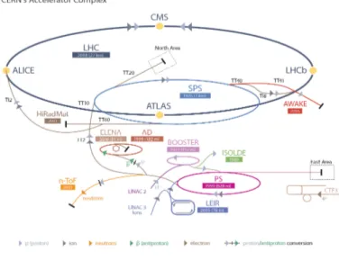
Particle injection in LHC is done employing pre-existing accelerators, following those steps:

• Protons are injected inside the Linear Accelerator LINAC2, that makes them reach 50 Mev;

• then particles pass through the Booster reaching 1.4 Gev;

• in the Proton Sychrotron (PS) protons are accelerated up to 0.99c, thus reaching 25GeV;

• the Super Proton Synchrotron (SPS), which is a sub-ring of 7 Km, makes the particles reach 450 GeV;

• the beam is finally injected into the LHC ring, where it gets accelerated up to the final center-of-mass energy of 13 TeV.

Figure 1.1: LHC Complex

The LHC beam filling requires about two hours. The beam lifetime is about 22 hours, however data are usually taken only in the first 10 hours, then the beams are dumped and a new fill is started in order to restart at maximum beam intensity to maximize the integrated luminosity collected by the detectors. Beams have a bunched structure with a crossing frequency f = 40MHz, corresponding to a time between collisions of 25ns.

(11)

Bunches contains about N = 1.1 · 1011 _{protons each.}

There are seven experiment currently installed at LHC, four of which are considered the main ones:

• ALICE is a detector whose goal is to study heavy ion colisions giving special atten-tion to Quark-Gluon plasma phenomena and the restoraatten-tion of the chiral symmetry.

size 26m(length), 16m(height), 16m(width)

weight 10000 tons

location Sergy (France)

• ATLAS is a multipurpose detector able to cover a wide variety of phenomena from high precision measurements to the discovery of new physics.

weight 7000 tons

location Meyrin(Switzerland)

• CMS detector is another multi-purpose detector with a very different technical design with respect to ATLAS. Further informations will be given in Chapter 2.

weight 12500 tons

location Cessy (France)

• LHCb is specialized in studying the asymmetry between matter and anti-mater in processes involving particles containing b quark.

weight 5600 tons

(12)

1.2 Physics at the Large Hadron Collider

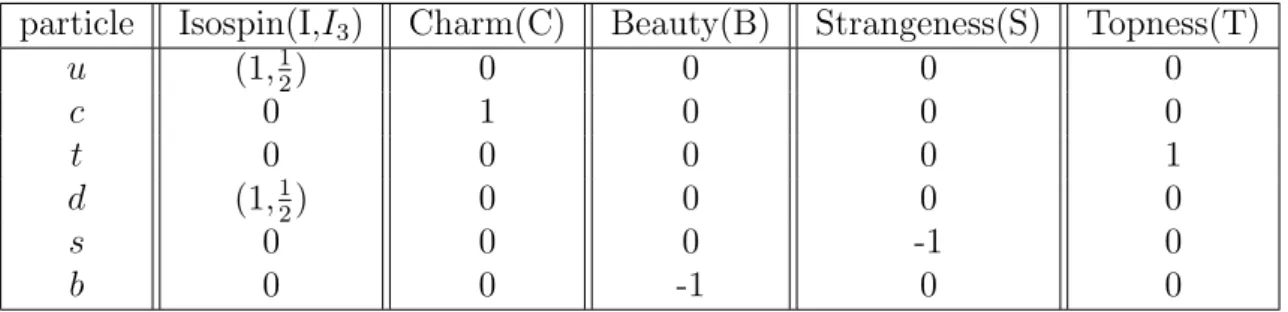
The Standard Model (SM) is currently the most advanced theory we can use to de-scribe the complex nature of subnuclear phenomena. Starting from a small cluster of particles and three fundamental forces, mathematically expressed via Gauge theory, the SM provides an accurate description of particle physics.

Figure 1.2: Standard Model

The particles in the SM can be split in two macro-groups: Fermions and Bosons. Fermions obey to Fermi-Dirac Statistics and, most importantly, Pauli’s exclusion prin-ciple. Bosons, on the other hand, obey to the Bose-Einstein Statistics. This difference will have, for instance, crucial consequences in the mathematical treatment of nuclei. Focusing on Fermions, we can split them into two further families: Leptons and Quarks. Leptons (e,µ,τ ) have unitary charge, defined in terms of single electron charge (e =

1.6 · 10−13C) and they interact only via the Electromagnetic force. There are three other

leptons, namely the three types of Neutrino(νe; νµ; ντ) whose charge is strictly zero and

the interaction they undergo is only the Weak one. Each Lepton has its own AntiLep-ton, this latter being a particle with same mass as the former but endowed with opposite electric charge.

Particle Mass(MeV) Charge(e)

e 0.5 -1 µ 106 -1 τ 1770 -1 νe < 2 · 10−6 0 νµ < 0.19 · 10−6 0 ντ < 18.2 · 10−6 0

(13)

Quarks (u,c,t,d,s,b) are subject to all the SM interactions and have half integer charge (see table 1.2). We can classify these particles introducing a new quantum number called flavour; for more details see Table 1.3.

Each Quark has its own AntiQuark, a particle with same mass but opposite electric charge.

Quarks have not been directly observed since a well comprehended property of their nature, namely “Confinement”, makes apparently impossible to disengage and isolate a single Quark.

Thus, only bound states of Quarks, expressely Hadrons, have been observed.

We can split the whole Hadron family in two branches: Mesons and Baryons, their dif-ference being in the internal composition.

Mesons are in fact composed by a Quark-AntiQuark couple whereas Baryons are formed by a triplet of Quarks or AntiQuarks.

particle Mass(MeV) Charge(e)

u 350 2₃ c 1500 2₃ t 180000 2 3 d 350 -1₃ s 500 -1₃ b 4500 -1 3

Table 1.2: Masses and charges of Quarks.

particle Isospin(I,I3) Charm(C) Beauty(B) Strangeness(S) Topness(T)

u (1,1₂) 0 0 0 0 c 0 1 0 0 0 t 0 0 0 0 1 d (1,1₂) 0 0 0 0 s 0 0 0 -1 0 b 0 0 -1 0 0

Table 1.3: Classification of Quarks via Flavour quantum numbers.

We shall now take a closer look to interactions.

In Nature, four interactions are known to exist: Gravitational, Strong, Weak and Elec-tromagnetic. The SM, by the way, is able to provide a quantitative description only as far as the last three are taken into account. The mathematical frame used to do so is the Gauge theory.

Basically the main idea behind Gauge theory is the following: taking into account a given system, its Lagrangian is written down and its symmetries, which are valid in each

(14)

point of the space (global symmetry), get tracked down. Then, an Ansatz is made: the Lagrangian should have also local symmetries which can be deduced from the global ones.

Thus we introduce a gauge field whose property is to correctly couple particles to fields. The symmetry underlying the SM, expressed in group formalism, is the following:

SU (3) × [SU (2) × U (1)]

The dimension of each representation is connected to the number of charges involved in the interaction.

SU(3) represents the Strong interaction and predicts three charges, which happen to be the colour charges (red, blue, green) of Quarks, and eight fields, that correspond to

Gluons1.

SU(2) is connected to the Weak interaction and correctly predicts two charges involved,

the Isospin couple, and three fields (Z0_{; W}± _bosons).

U(1) represents the Electromagnetic interaction and only one charge is theoretically needed.

1.2.1 Beyond the Standard Model

The Standard Model of particle physics agrees very well with experiments, but many physical phenomena in nature are not adequately explained. For example the SM does not explain gravity. The approach of simply adding a “ graviton ” to the theory does not account what is observed experimentally. On the other hand, the SM cannot be included in the most successful Einstein’s theory of general relativity.

Another problem which the SM does not answer to is the precence of dark matter. Cosmological observations tell us the standard model explains about 5% of the energy present in the universe. About 26% should be dark matter which only interacts weakly with the Standard Model fields. Yet, the SM does not supply any fundamental particles that are consistent dark matter candidates.

The remaining 69% of the energy in the universe should be so called “ dark energy ”, a constant energy density for the vacuum. Attempts to explain dark energy in terms of vacuum energy of the SM lead to a mismatch of 120 orders of magnitude.

As we can see from figure 1.3, neutrinos are massless particles in the context of the Standard Model. However neutrinos oscillation experiments have shown that neutrinos do have mass. Mass terms can be added to the theory “ by hand ”, but this lead to new theoretical problems. For instance, the mass terms need to be extrimely small and it is not clear if the neutrino masses would arise in the same way as the masses of other

1_{This is obtained following Yang-Mills theory. Given a representation dimension N, the number of}

(15)

Figure 1.3: Physics beyond the Standard Model

fundamental particles do in the Standard Model.

Finally there is the crucial problem of matter-antimatter asymmetry. The Universe is made out of mostly matter. However, the standard model predicts that matter and antimatter should have been created in equal ammounts if the initial conditions of the universe did not involve disproportionate matter relative to antimatter. Yet, no mech-anism to explain this asymmetry exists in the Standard Model. It is because of these unsolved problems that experimental physicists continue to upgrade and improve exper-iments to investigate nature.

(16)

Chapter 2 The Compact Muon Solenoid

experiment

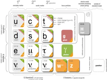
The Compact Muon Solenoid (CMS) detector at CERN LHC is a general purpose device designed to search for signatures of new physics in proton-proton and heavy ion colisions. Since many of these signatures include muons, CMS is constructed with subdetectors to identify muons, trigger the CMS readout upon their detection, and measure their momentum and charge over a broad range of kinematic parameters.

Figure 2.1: The Compact Muon Solenoid

Kinematics in CMS is described according to a right-handed coordinate system where the origin is placed in the p-p interaction point. The z axis is along the beam pipe, the

(17)

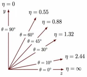
abscissa points at the centre of LHC and the ordinates points upwards. Polar coordinates (R,θ,φ) are often used to describe kinematics of collision products. The polar angle θ is defined in the zy plane, while the azimuthal angle φ is defined in the xy plane. In this latter the track bending in the magnetic field happens and the momentum component on

this plane is called transverse momentum pT. Another significal parameter, often used

in collider physics, is the rapidity defined as

y = −1

2ln

E + pz

E − pz

(2.1) since it is invariant for Lorentz boost. Considering that rapidity depends on quantities that can’t be directly measured,a further crucial parameter is the pseudorapidity defined as

η = −1

2ln

θ

2 (2.2)

Pseudorapidity approximates rapidity in the ultra relativistic regime.

Figure 2.2: Pseudorapidity range

2.1 The CMS detector

The CMS detector has a cylindrical geometry with several concentric layers of com-ponents [1]. The innermost element of the detector is the Silicon Tracker which records paths taken by charged particles, bended by the 3.8T magnetic field produced by the solenoid magnet, finding their positions at a number of key points. The tracker can

(18)

reconstruct paths of high-energy muons, electrons and hadrons as well as see tracks com-ing from the decay of very short-lived particles. In view of this variety of particles the detector includes two kinds of calorimeters. The Electromagnetic Calorimeter (ECAL), the internal layer of the two, measures the energy of electrons and photons by stopping them completely. Conversely hadrons, made up by quarks and guons, fly through the ECAL and are stopped by the outer layer called the Hadron Calorimeter (HCAL).

Figure 2.3: CMS components

As previously mentioned, CMS main goal is to detect muons, which can penetrate several metres of iron without interacting, unlike most of particles that are stopped

by calorimeters. Therefore, the muon system is located outside the solenoid and it

is composed of gaseous detectors, interposed among the layers of the steel flux-return yoke, that allow a traversing muon to be detected at multiple points along the track path. Muon system is composed of three types of gas ionization chambers, DT, CSC and RPC. The drift tubes chambers (DT) are segmented into drift cells so the position of muons is determined by measuring the drift time to an anode wire of a cell with a shaped electric field. The cathode strip chambers (CSC) operate as standard multi-wire proportional counters but add a finely segmented cathode strip readout, which yelds an accurate measurement of the postion of the bending plane (R-φ) coordinate at which

the muon crosses the gas volume. The resistive plate chambers (RPC) are

double-gap chambers operated in avalanche mode and are primarly designed to provide timing information fot the muon trigger. The DT and CSC chambers are located in the regions |η| < 1.2 and 0.9 < |η| < 2.4 respectively, and are complemented by RPCs in the range

(19)

|η| < 1.9. Three regions can be distinguished, naturally defined by cylindrical geometry of the detector, referred to as the barrel |eta| < 0.9, overlap 0.9 < |η| < 1.2 and endcap 1.2 < |η| < 2.4 regions. In the barrel a station is a ring of chambers assembled between two layers of the steel flux-return yoke at approximately the same value of radius R. There are four DT and four RPC stations in the barrel, labeled MB1-MB4 and RB1-RB4, respectively. Conversely in the endcaps a station is a ring of chambers assembled between two disks of steel flux-return yoke at approximately the same value of z. There are four CSC and four RPC stations in each endcap, labelled ME1-ME4 and RE1-RE4, respectively. Between Run1 and Run2 additional chambers were added in ME4 and RE4 to increase redundancy, improve efficiency and reduce misidentification rates.

2.1.1 The Drift Tube chambers system

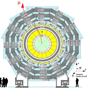
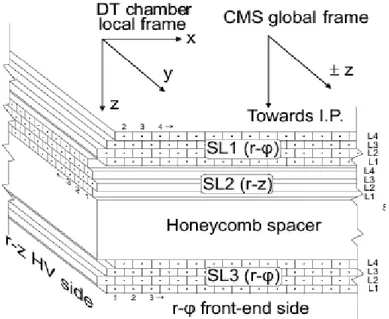
In the barrel region the muon rate is low, the neutron background is relatively small except in the outermost station MB4 and the magnetic field is mostly uniform with strength below 0.4T in between the yoke segments. Here drift chambers with standard rectangular cells and electrical field shaping are employed. The DT detector is composed by 5 wheels along the beam direction (z). They are called “YB ”(Yoke Barrel) and are organized into 12 φ−segments per wheel, forming four stations at different radii inter-spersed between plates of the magnetic flux return yoke called MB1-MB4. Each station consists of eight layers of tubes measuring the position in the bending plane and four layers in the longitudinal plane.

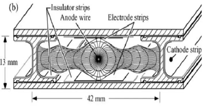
The basic element of the DT system is the drift cell which has a transverse size of

42 × 13mm2 with a 50µm diameter gold-plated stainless steel anode wire at the

cen-ter that operates at +3600 V. The gas mixture(85%/15% of Ar/CO2) provides good

quenching properties and a saturated drift velocity of about 55µm/ns. The maximum drift time is almost 400ns. The cell design uses four electrodes to shape the effective drift field, two on the side walls of the tube and two above and below the wires on the ground planes between the layers. Four staggered layers form a superlayer (SL), while a chamber consists of two superlayers that measure the r − φ coordinates with wires parallel to the beam line, and a othogonal superlayer that measures the r − z coordinate. This is except from the MB4 which has only an r − φ superlayer.

Chambers are limited in size in the longitudinal direction by the segmentation of the barrel yoke and are about 2.5 m long. On the transverse size their lenght varies with the station ranging from 1.9 m, for MB1, to 4.1 m for MB4.

The DT and CSC muon detector elements together cover the full CMS pseudorapidity interval |η| < 2.4 with no acceptance gap, ensuring good muon identification over a

range corresponding to 10◦ < θ < 170◦. Offline reconstruction efficency for the muons

(20)

Figure 2.4: CMS azimuthal view

transition region between the barrel outer wheels and the endcap disks. The amount of absorbing material before the first muon station reduces the contribution of punch-through particle to about 5% of all muons reaching the first station and to about 0.2% of all muons reaching further muon stations. Crucial properties of the DT system are that it can identify the collision bunch crossing that generated the muon and trigger on

the pT of muons with good efficiency and that it has the ability to reject background by

means of timing discrimination. The DT system calibration

Charged particles, crossing a drift cell in the DTs, ionize the gas in the cell. The drift time of the ionization electrons is obtained by using a time-to-digital converter (TDC), after substracting a time pedestal. This latter contains contributions from the latency of the trigger and from the propagation time of the signal within the detector and the data acquisition chain. The hit position is reconstructed as

xhit = tdrif t· vdrif t = (tT DC − tped) · vdrif t (2.3)

where tT DC is the measured time, tped the time pedestal, and vdrif t the effective drift

velocity, which we assume being approximately constant in the cell volume [2].

In an ideal cell the time distribution from the TDC would have a box shape starting at close to 0 ns for muon tracks passing near the anode and extending up to 380 ns for

(21)

Figure 2.5: DT layers and superlayers

those passing close to the cathode. In practise different time delays related to the trigger latency and the length of the cables to the readout electronics contribute to the time measured by the TDC:

tT DC = tdrif t+ twire0 + tL1+ tT OF + tprop (2.4)

where the different contributions to the time pedestal are classified as

• twire

0 , the channel by channel signal propagation time to the readout electronics,

relative to the average value in a chamber ; it is used to equalize the response of all the channel in a chamber;

• tL1, the latency of the Level-1 trigger;

• tT OF, the time of flight of the muon produced in a collision event, from the iteraction

point to the cell;

• tprop, the propagation time of the signal along the anode wire.

The inter-channel synchronisation twire₀ is determined by test pulse calibration runs. It is

a fixed offset since it depends only on the cable lenght. The remaining contribution to the time pedestal is extracted from the data for each SL. It is computed as the turn-on point of the TDC time distribution , after correction for the inter-channel synchronisation.

(22)

Figure 2.6: Section of a drift tube cell

includes the contributions from the average time-of-flight, as well as the average signal propagation time along the anode wire, taken from the centre of the wire to the front-end board. The correction for the propagation time along the wire and the muon time-of-flight to the cell is performed at the reconstruction level, after the 3D position of the track segment is determined. Finally to define the turn-on point of the TDC time distributions

more precisely, a correction to the ttrig pedestal is calculated by using the hit position

residuals. These latter are computed as the distance between the hit position and the intersection of the 3D segment with the layer plane.

The drift velocity depends on the gas mixture, purity and the electrostatic configuration of the cell. The effective drift velocity is further affected by the presence of the residual magnetic field and the track incidence angle and is computed as an average for each SL system. To determine the drift velocity we use two methods where the first is based on the “ mean-time ” tecnique and the second is based on the local muon reconstruction in which a track is fitted to measurements from one chamber at a time. The mean-time method exploits the staggering of the chamber layers. Because of the staggering, ionization electrons drift in opposite directions in even and odd layers. Therefore the

maximum drift time tmaxin a semi-cell can be calculated from the drift times of hits from

the track crossing nearby cells in consecutive layers. The appropriate mean-time relation is chosen for each track by using the three-dimensional position and direction of the track segment in the SL. To determine the drift velocity we use the linear approximation

vef f_{drif t}= Lsemi−cell/ < tmax > (2.5)

where Lsemi−cell = 2.3mm is approximately half the width of a drift cell.

An alternative method for computing the drift velocity relies on the full reconstruction of the trajectory in the muon system. A track is reconstructed by assuming the nominal drift velocity and in a second step is refitted with the drift velocity and the time of passage of the muon through the chamber as free parameters. This method is applied to the r − φ view of the track segment in a chamber, but cannot be applied to the r − z

(23)

SLs where only four points are available in the fit to disentagle the drift velocity and synchronisation contributons. Finally a notable reduction of drift velocity of about 2% is observed in the innermost chambers of the outer wheels because of the Lorentz angle induced by the stronger magnetic field.

2.2 Muon Triggering and Reconstruction

2.2.1 The Trigger system

The triggering scheme of the CMS muon system relies on two indipendent and com-plementary triggering technologies, one based on the precise tracking detectors in the barrel and endcaps, and the other based on the RPCs. The tracking detectors provide exellent position and time resolution, while the RPC system provides exellent timing but with poorer spatial resolution.

For values of the transverse momentum pT up to 200 GeV/c, the momentum resolution

is dominated by the large multiple scattering in the steel, combined in the endcaps with the effect of the complicated magnetic field that is associated with the bending of the field lines returning through the barrel yoke.

The large number of layers in each tracking chamber is exploited by a trigger hardware processor that constructs tracks segments in the chambers with a precision sufficient to set sharp transverse momentum thresholds at the level-1 trigger level up to 100GeV/c, and to tag the parent bunch crossing (BX) with very good time resolution. This com-ponent of the L1 trigger is called the “ local trigger ” since it operates purely with information local to a chamber.

Originally the Muon Trigger was designed to preserve the complementarity and redun-dancy of CSC, DT and RPC which were used to build tracks separately until they were combined in the Global Muon Trigger.

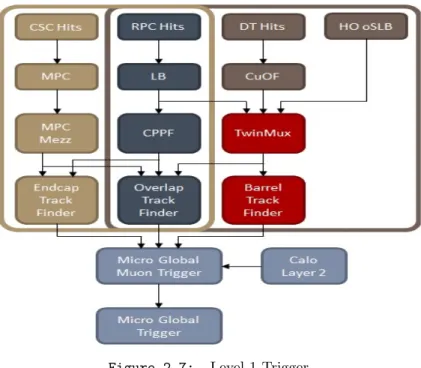
Now all the hits contribute to the track whatever subsystem detects them. Furthermore the upgrade introduced a regional segmentation that treats muon tracks separately de-pending on η. It distinguishes a barrel region(low η), an endcap region (high η) and a transition region between them (|η| ≈ 1) called overlap. Such regions result in different triggering algorithms but also in different deployments of hardware processors. The final sorting and ghost track cancellation of muon candidates are hanled separately for each of the three regions in η. Finally all the informations are sent to the Global Trigger which takes the final decision wether to reject or accept the event, based on a menu of hundreads of different decision algorithms, tuned for different physics cases.

(24)

Figure 2.7: Level 1 Trigger

A suitably steep transverse momentum treshold is obtained by requiring a local spatial resolution of the segments on the order of a couple of millimetres. This resolution is necessary to guarantee a high trigger efficiency and defines a lower limit on the accurancy that must be reached by the alignment of the chamber positions.

2.2.2 Muon reconstruction

The geometry of CMS has a deep influence on the performance of the muon system. The change in the direction of the magnetic field in the return yoke causes the curvature of the muon trajectory to reverse. Therefore the first muon detector stations, in both the barrel and endcap regions, are critical since they provide the largest sagitta and hence the most important contribution to the measurement of the momentum of high momenta muons, for which multiple scattering effects become less significant.

Reconstruction proceeds by first identifying hits in the detection layers of a muon cham-ber due to the passage of a muon or another charged particle, and in the DT and CSC systems by then building straight-line track segments from these hits. Local reconstruc-tion in DT chambers is performed in steps [3]:

• drift time is converted in a drift distance from a wire in a DT cell;

• cell hits are used to fit 2D segments indipendently in r − φ (up to 8 hits) and r − z superlayers (up to 4 hits);

(25)

• the two projection are combined to build a 3D segment in the chamber which will be used in the track fit

This is referred to as local reconstruction. The reconstruction of muon tracks from these hits and segments is called global reconstruction. Muon tracks can be reconstructed by using hits in the muon detectors alone so the resulting muon candidates are called stan-dalone muons. Alternatively the reconstruction can combine hits in the muon detectors with those in the central tracker and the resulting muon candidates are called global muons. Finally the muon system can also be used purely to tag extrapolated tracks from the central tracker which are called “tracker muons ”.

At large transverse momenta, pT > 200 GeV, the global-muon fit improves the

momen-tum resolution with respect to the tracker-only fit, but as the pT value increases, the

additional hits in the muon system gradually improve the overall resolution. Global muons exploits the full bending of the CMS solenoid and return yoke to achieve the ultimate performance in the Tev/c region.

Figure 2.8: Reconstruction of a muon trajectory

Reconstructed muons are fed into the CMS particle flow (PF) algorithm. This latter combines information from all CMS subdetectors to identify and reconstruct all individ-ual particles for each event, including electrons, neutral hadrons, and muons. For muons PF applies a set of selection criteria to candidates reconstructed with standalone, global or tracker muon algorithms.

(26)

Chapter 3 Background studies

Levels of background radiation in the CMS muon system can in principle affect its overall performance. Any background source, including low energy neutrons or photons, electrons and positrons, punch-through hadrons, low momentum primary and secondary muons, and in general all beam-induced background could affect the muon trigger per-formance and pattern recognition of muon tracks. In particular, spurious hits produced by noise or radiation background could spoil the track reconstruction and promote low transverse-momentum muons to higher momentum. Furthermore the radiation back-ground could affect the detector performance by accelerating the CMS aging and there-fore its efficiency degradation.

3.1 Measurement tecniques

Each of the muon subsystems employ different technology and different materials, thus each one responds differently to the various backgrounds. For example, on one hand, the CSC system has six active planes per chamber and typically requires at least four out of six hits to generate a track segment. Hence, the CSCs are relatively immune to neutrons, which generally affect only a single plane. On the other hand, the CSCs cannot distinguish punch-through background particles from genuine muon tracks. The RPC system provides a single hit per chamber from two gaps, and thus it triggers on neutron hits. However, the RPC system has a very narrow time window of 25 ns and is relatively uneffected by out-of-time signals. Finally the DT system has twelve planes per chamber and the segment reconstruction is mostly immune to neutron hits as long as the rate is not too high. The time window for the DTs, however, is large that so it suffers from out-of-time background, hence high background rate could make track reconstruction difficult, and the event size could become too large for the readout. As a result of these different technologies, each subsystem measures background rates in a different manner. The CSC system measures the trigger rate per chamber. To increase

(27)

the sensitivity to background such as neutrons, the CSC trigger was to run in a special configuration that requires only a single layer coincidence of wire and strip hits within a time window of 75 ns. A coincidence of two or more hits from different layers that satisfy the single track criteria is considered in this configuration as a single triggering event.The RPC average strip rate is calculated by using the incremental counts, perfrmed at the level of the RPC DAQ board, normalized to the strip area. The noise level is estimated of each run and each chamber separately through a linear extrapolation to a value for an istantaneous luminosity at 0, which is then subtracted from the chamber rate. After this noise subtraction, the resulting RPC rate is divided by two to account for the two RPC gaps.

Further informations about DTs will be given in the following paragraph.

3.2 Background in the DT chambers

The DTs consider as background detector signals that aren’t produced by crossing muons. By integrating over the full 1.25 µs readout window, the DTs also measure rates of out-of-time background originating mainly from slow neutrons, hadron punch-through, and hits that originated from other bunch-crossings (pileup). As shown in Figure 3.1, the time distribution of these hits in the full 1.25 µs TDC time window is flat, in contrast to the one for signals generated by prompt muons from proton-proton collisions, which arrive roughly within a 400 ns time interval, corresponding to the drift time across an entire cell. 0 200 400 600 800 1000 1200 1400 time [ns] 0 0.002 0.004 0.006 0.008 0.01 0.012 0.014 0.016 0.018 A.U.

Signal and Background digi time distribution

(28)

The background observed in the DT chambers has two different origins

• The so called “ neutron gas ” which is produced by colliding beams and fill the empty space between the detector and the caver’s ceiling. It is mainly responsible for the background in the external stations (MB4) of the upper sectors;

• The high particle multiplicity in the forward regions related to Pile Up: hadron punch-through and shower leaks are some of the causes of background in the in-ternal stations (MB1), mainly in exin-ternal wheels.

(29)

Chapter 4 Study of DT reconstructed

background segments

Our main goal was to assess the origin of background which affects the DT stations. In the Run 1, study any superlayer with more than two recorded hits was discarded as being potentially crossed by a prompt muon. Furthermore in the Run1 study, only the 0 - 250 ns time range was considered for the background computation. This method is suitable to study hit background but (by definition) it can’t be used to study segments. On the other hand reconstructed track segments in the muon susbsystems are used to seed the muon reconstruction. Therefore monitoring background segments is crucial. For this reason we started from the approach of considering as background whatever signal is not produced by a crossing muon [6]. In order to preserve sensitivity for different types of background, the new approach consists of a tighter definition of the muon signal region and, as a consequence, a larger acceptance for background.

Now we accept as background whatever hits or reconstructed segments are found within the chambers that were not crossed by reconstructed muons, and within in the full range readout by the TDC which is 1275 ns.

4.1 Main tools used for the analysis

The whole analysis was developed using the Root framework.

Root-ples were produced starting from CMS data, in the standard format of the “ DT Tree ”, used by the DT group. This tree contains all relevant information for muon detector performance studies. For our analysis we needed information related to:

• reconstructed muons, to define the signal regions to be discarded;

(30)

The muon related information that was relevant to our analysis was the list of DT chambers crossed by the muon trajectory: this was only defined for reconstructed muons that exploit the tracker information, by means of propagating the inner track to the muon stations. For what concerns standalone-muons, the list of DT segments associated in the muon reconstruction was used instead to identify the chambers to be descarded before background computation. So for every event a loop on the reconstructed muons is performed and the list of crossed chambers is registered. Having identified event by event the remaining chambers to be considered for the background evaluation, we looked at hits and segments (if any) detected within them.

4.1.1 Dataset used

Full event information with both raw and reconstructed data requires several MBytes of disk space per event. Therefore it is impossible to store it for all events registered by CMS, but some datasets have this informations saved for specific need of the analysis groups. Among these, the groups in charge of studying the performance of the muon detectors make use of the so called “ZMu Skim” data: sets of events triggered by a “Single muon trigger” and then selected for containing a candidate Z boson decaying into a pair of muons. The results shown in the following sections have been obtained using nearly five milions events of the ZMu Skim collected by CMS between August 28 to September 6, 2018.

4.2 Analysis workflow

4.2.1 One-dimensional study

In order to identify the origin of the background segments we first propagated them as straight lines in the z − R plane and found the intersection with the z axis (beam line). In the z − R view there is no bending of the tracks. Since we needed positions and directions for all three coordinates in the CMS global reference frame, we could only use segments that are reconstructed in both the transverse and longitudinal views. Thus, this analysis is performed only for the first three stations (MB1, MB2, MB3), as the chambers of the MB4 station have no theta Superlayer, therefore they provide no z measurements (see Section 4.2.4).

For each fully reconstructed segment, in the three inner stations, its coordinates and its director cosines are available. Such information is used to determine a straight line in the z − R plane containing the segment position and the beam line. With some basic trigonometry, we determine the z coordinate of the intersection of the straight line derived from the segment with the z axis.

(31)

• for each segment position, we calculate its distance from the z-axis

r⊥ =

q x2

S+ yS2, (4.1)

where xS and yS are the coordinates of the segment in the transverse plane, in the

global reference frame;

• the angle between the segment direction and the z axis (see Figure 4.1) is defined by the relation

tan θS =

r⊥

zS− zL

, (4.2)

where θS is obatined by the arc cosine of the z director cosine;

• we extract the value zL, as

zL= zS− r⊥ tan θS (4.3) 0 2 4 6 8 10 12 z (m) R ( m ) 1 0 2 3 4 5 6 7 8 1 3 5 7 9 11 5.0 4.0 3.0 2.5 2.4 2.3 2.2 2.1 2.0 1.9 1.8 1.7 1.6 1.5 1.4 1.3 1.2 1.0 0.9 1.1 0.8 0.7 0.6 0.5 0.4 0.3 0.2 0.1 40.4° 44.3° 36.8° 48.4° 52.8° 57.5° 62.5° 67.7° 73.1° 78.6° 84.3° 0.77° 2.1° 5.7° 9.4° 10.4° 11.5° 12.6° 14.0° 15.4° 17.0° 18.8° 20.7° 22.8° 25.2° 27.7° 30.5° 33.5° θ° η θ° η ME4 /1 ME3 /1 ME2 /1 ME1 /2 ME1 /1 ME2 /2 ME3 /2 ME1 /3 R E3 /3 R E1 /3 R E1 /2 MB1 MB2 MB3 MB4 Wheel 0 Wheel 1 RB1 RB2 RB3 RB4 Solenoid magnet Silicon tracker Steel Wheel 2 R E2 /3 R E3 /2 ME4 /2 R E4 /3 R E4 /2 R E2 /2 CSCs RPCs DTs R E2 /2 HCAL ECAL zS zL r⟂ θS segment z

(32)

1000 − −500 0 500 1000 z [cm] 0 0.05 0.1 0.15 0.2 0.25 0.3 0.35 A.U.

MB1 segments extrapolation to beam line

Figure 4.2: MB1 segments extrapolation to beam line 1000 − −500 0 500 1000 z [cm] 0 0.05 0.1 0.15 0.2 0.25 0.3 0.35 0.4 0.45 A.U.

Figure 4.3: MB2 segments extrapolation to beam line 1000 − −500 0 500 1000 z [cm] 0 0.1 0.2 0.3 0.4 0.5 A.U.

Figure 4.4: MB3 segments extrapolation to beam line

In Figures 4.2, 4.3, 4.4, the distribution of values of zL is shown, for signal and

background segments. Here we have superimposed the signal histogram (blue) to the background histogram (red) for each station, normalizing them to each other, for MB1, MB2, MB3 respectively.

4.2.2 Two-dimensional study

We can see that while signal segments precisely point to the region around z ≈ 0, corresponding to the interaction point, background has two bumps approximately at -400 and +400 on the z axis which roughly correspond to the position of the calorimeter cracks. However we couldn’t say precisely were the origin of the tracks actually was. In order to visualize it, we built a two-dimensional histogram to be filled with the straight

(33)

lines extrapolated from the segment positions and angles: we expect that entries in this histograms will accumulate around the region where tracks are produced. For every value “ i-th ” of the radius we calculated its corresponding value of z as follows

r⊥,i = r⊥− ri (4.4)

zL= zS−

r⊥,i

tanθ (4.5)

and for each (r⊥,i, zL,i) pair we filled the corresponding bin of the histogram.

4.2.3 Results

In Figures 4.5, 4.6 and 4.7,the distribution of straight lines described in the previous paragraph is shown for signal segments. As expected, the most occupied regions of are located at (r,z)=(0,0) for signal segments, consistent with the fact that the corresponding tracks are originated at the interaction point.

1000 − −500 0 500 1000 z [cm] 0 100 200 300 400 500 600 700 800 R [cm] 0 100 200 300 400 500 600 700 800 900 3 10 × Signal segments in MB1

Figure 4.5: R − z plot of line densi-ties for signal segments in MB1

1000 − −500 0 500 1000 z [cm] 0 100 200 300 400 500 600 700 800 R [cm] 0 100 200 300 400 500 600 700 800 3 10 × Signal segments in MB2

1000 − −500 0 500 1000 z [cm] 0 100 200 300 400 500 600 700 800 R [cm] 0 100 200 300 400 500 600 700 3 10 × Signal segments in MB3

In Figures 4.8, 4.9, 4.10 we can see the straight line trajectory of background seg-ments. In all three histograms the CMS geometry is clearly visible. For instance,at

(34)

the radius value which corresponds to the station position, we can see four low density regions that correspond to the gaps between consecutive wheels where no segment can be reconstructed (see Figure 4.11).

1000 − −500 0 500 1000 z [cm] 0 100 200 300 400 500 600 700 800 R [cm] 0 5000 10000 15000 20000 25000 30000 Background segments in MB1

Figure 4.8: Background segments in MB1

1000 − −500 0 500 1000 z [cm] 0 100 200 300 400 500 600 700 800 R [cm] 0 500 1000 1500 2000 2500 3000 Background segments in MB2

1000 − −500 0 500 1000 z [cm] 0 100 200 300 400 500 600 700 800 R [cm] 0 100 200 300 400 500 600 700 Background segments in MB3

In Figure 4.8, where MB1 stations are shown, we can see two outstanding accumu-lations at about -500 cm and 500 cm on the z axis and between 400 cm and 300 cm on the R axis which are supposed to be the origins of background segments. Even if we are considering background segments, some of them are found to point to the interaction point.

In Figure 4.9 the distribution is different. Actually in MB2 stations the accumulations are at larger radius and there are more background segments that point to the origin. Finally in Figure 4.10 we can see that MB3 shows more tracks coming from the inter-action region and none at |z| ≈ 500cm It should be noticed that the maximum of the

(35)

1000 − −500 0 500 1000 z [cm] 0 100 200 300 400 500 600 700 800 R [cm] 0 5000 10000 15000 20000 25000 30000 Background segments in MB1 0 2 4 6 8 10 12z (m) R ( m ) 1 0 2 3 4 5 6 7 8 1 3 5 7 9 11 5.0 4.0 3.0 2.5 2.4 2.3 2.2 2.1 2.0 1.9 1.8 1.7 1.6 1.5 1.4 1.3 1.2 1.0 0.9 1.1 0.8 0.7 0.6 0.5 0.4 0.3 0.2 0.1 40.4° 44.3° 36.8° 48.4° 52.8° 57.5° 62.5° 67.7° 73.1° 78.6° 84.3° 0.77° 2.1° 5.7° 9.4° 10.4°11.5° 12.6° 14.0° 15.4° 17.0° 18.8° 20.7° 22.8° 25.2° 27.7° 30.5° 33.5° θ° η θ° η ME4 /1 ME3 /1 ME2 /1 ME1 /2 ME1 /1 ME2 /2 ME3 /2 ME1 /3 R E3 /3 R E1 /3 R E1 /2 MB1 MB2 MB3 MB4 Wheel 0 Wheel 1 RB1 RB2 RB3 RB4 Solenoid magnet Silicon tracker Steel Wheel 2 R E2 /3 R E3 /2 ME4 /2 R E4 /3 R E4 /2 R E2 /2 CSCs RPCs DTs R E2 /2 HCAL ECAL 0 2 4 6 8 10 12 z (m ) R ( m ) 1 0 2 3 4 5 6 7 8 1 3 5 7 9 11 5.0 4.0 3.0 2.5 2.4 2.3 2.2 2.1 2.0 1.9 1.8 1.7 1.6 1.5 1.4 1.3 1.2 1.0 0.9 1.1 0.8 0.7 0.6 0.5 0.4 0.3 0.2 0.1 40.4° 44.3° 36.8° 48.4° 52.8° 57.5° 62.5° 67.7° 73.1° 78.6° 84.3° 0.77° 2.1° 5.7° 9.4° 10.4° 11.5 ° 12.6° 14.0° 15.4° 17.0° 18.8° 20.7° 22.8° 25.2° 27.7° 30.5° 33.5° θ° η θ° η ME4 /1 ME3 /1 ME2 /1 ME1 /2 ME1 /1 ME2 /2 ME3 /2 ME1 /3 R E3 /3 R E1 /3 R E1 /2 MB1 MB2 MB3 MB4 Wheel 0 Wheel 1 RB1 RB2 RB3 RB4 Sole noi d m agn et Silic on trac ker Steel Wheel 2 R E2 /3 R E3 /2 ME4 /2 R E4 /3 R E4 /2 R E2 /2 CSC s RPC s DTs R E2 /2 HCAL ECA L

Figure 4.11: Superposition of the MB1 histogram with CMS z − R section

color scale in the three plots is different from each other. Indeed in MB1 the maximum density value is 30 000, while in MB2 is 3000, and finally in MB3 is 700.

MB1 stations have a very high background which comes from the calorimeter cracks: particles passing through the cracks interact in the solenoid or in the iron yoke, forming the accumulation visible in Figure 4.8. In MB2 stations, we see particles which passed through the cracks but didn’t interact before the second iron layer of the yoke between MB1 and MB2. In fact, their density is lower.

Finally, the acceptance of MB3 stations does not cover the cracks and so the two accumu-lations are no more visible. Another source of background seems to be in the calorimeter, around z=0: it is well visible in the MB3 (Figure 4.10), less in the MB2 (Figure 4.9) and not at all in the MB1 (Figure 4.8), due to the different color scale.

Finally in all three stations there is a component which comes from the interaction point. These could be segments belonging to muons which were not reconstructed properly or to prompt muons from a different bunch crossing. To verify the hypothesis, we reproduced the graphics dividing in-time from out-of-time segments. Each reconstructed segment has a value of time, derived from the hit fit, referred to the collision time: a perfectly

timed segment will have tS ≈ 0. In order to define in-time segments, we apply a cut

on this value, |tS| ≤ 13 ns, while all segments not passing this cut are classified as

(36)

1000 − −500 0 500 1000 z [cm] 0 100 200 300 400 500 600 700 800 R [cm] 0 100 200 300 400 500 600 700 800 3 10 ×

In-time signal segments in MB1

Figure 4.12: MB1 in-time signal

1000 − −500 0 500 1000 z [cm] 0 100 200 300 400 500 600 700 800 R [cm] 0 1000 2000 3000 4000 5000 6000 7000

In-time background segments in MB1

Figure 4.13: MB1 in-time background

1000 − −500 0 500 1000 z [cm] 0 100 200 300 400 500 600 700 800 R [cm] 0 2000 4000 6000 8000 10000 12000 14000 16000 18000 20000 22000 24000 Out-of-time background segments in MB1

Figure 4.14: MB1 out-of-time background

In MB1 the ratio of entries of in-time background segments (Figure 4.13) and out-of-time background segments (Figure 4.14) is three. Histograms are slightly different from each other. In the out-of-time histograms there are more segments that point to the interaction point, which is consistent with the hypothesis that some of the segments classified as background correspond to prompt muons that could not be reconstructed because they were produced in out-of-time collisions.

(37)

1000 − −500 0 500 1000 z [cm] 0 100 200 300 400 500 600 700 800 R [cm] 0 100 200 300 400 500 600 700 800 3 10 ×

1000 − −500 0 500 1000 z [cm] 0 100 200 300 400 500 600 700 800 R [cm] 0 100 200 300 400 500 600

1000 − −500 0 500 1000 z [cm] 0 100 200 300 400 500 600 700 800 R [cm] 0 500 1000 1500 2000 2500

Out-of-time background segments in MB2

In MB2 stations the rate of entries of background in-time segments (Figure 4.16) and the entries of out-of-time segments (Figure 4.17) is about 0.27. Again in Figure 4.16 (in-time) we cannot see clear “paths” which point to the IP while, in Figure 4.17 (out-of-time) there is an accumulations near the interaction point.

(38)

1000 − −500 0 500 1000 z [cm] 0 100 200 300 400 500 600 700 800 R [cm] 0 100 200 300 400 500 600 3 10 ×

1000 − −500 0 500 1000 z [cm] 0 100 200 300 400 500 600 700 800 R [cm] 0 20 40 60 80 100 120 140

1000 − −500 0 500 1000 z [cm] 0 100 200 300 400 500 600 700 800 R [cm] 0 100 200 300 400 500 600

Out-of-time background segments in MB3

Finally, in MB3, we find that the rate of entries in the in-time background histogram (Figure 4.19) and in the out-of-time background histogram (Figure 4.20) is about 0.23. In figure 4.19 there is a light accumulation in the IP zone and some points at high density near the gaps between wheels suggesting that signal segments near the gaps failed to be associated to the reconstructed muon whose extrapolation likely passed in the gaps themselves. In Figure 4.20 similar patterns are visible, superimposed to a component originated in the calorimeter.

We can see that the rate of in-time background segments and out-of-time background segments decreases from MB1 to MB3.

Summarizing, we found that:

• some of the segments classified as background seems to be produced by prompt muons from out of time collisions, which are not reconstructed for this reason; • the contribution of out of time dominates in the outer stations, where the

(39)

ground rate is overall small; instead, it amounts to only 1/4 of reconstructed back-ground segments in MB1, where he backback-ground rate is larger;

• In MB3, also most of the in-time background seems to be due to segments related to prompt muons which were not reconstructed because of acceptance (escaping throug the gaps between the wheels).

4.2.4 Background in MB4 stations

The MB4 stations must be studied in a different way. This is because of two reasons. First, because of the lack of the θ Superlayer, the MB4 stations don’t reconstruct seg-ments in the z view.

Second, unlike the inner stations, in the MB4 stations we don’t expect background from the inside of the detector, but background produced by so called neutron gas and coming from above the detector.

Neutrons are originally produced by secondary interactions in the detector material and especially in the calorimeters. They diffuse outside like a gas, reach thermal energy and fill the empty space between the detector and the cavern ceiling. From there, they will randomly hit back the detector and, through nuclear capture, produce very soft electrons which in turn ionize the DT gas and give signals.

It is supposed that this mechanism is confined in one cell volume, but actually low quality segments are also reconstructed (Figure 4.21). The mechanism in under investigation. Two hypothetis were considered: segments could originate from casual alignments of background hits or they could be produced by electronics crosstalk.

Considering the first hypothetis we calculated the probability of the casual alignment of three hits.

We started from calculating the surface of the cell which is S=1023 cm2_{, hence the rate}

could be seen as S·R, where R=7Hz/cm2_{. Then, the average number of hits per event is}

rate·400ns, where 400ns is the drift time. Finally, using the Poisson distribution

Pλ(n) =

λn

n! exp{−λ}, (4.6)

we calculated the probability of a casual alignment of three hits and we found that this

(40)

0 1 2 3 4 5 6 7 8 9 10 Number of hits 0 50 100 150 200 250 300 350 400 3 10 × Entries Hits distribution in MB4

Figure 4.21: Number of hits associated to reconstructed background (red) and signal (blue) segments in MB4

We repeated the study performed with MB1, MB2, MB3 for the MB4, but this time on the R − ϕ plane. Only prompt muons with a high transverse momentum, and hence almost no bending arrive in MB4 stations as we can see from Figure 4.23. Background segments instead concentrates in the top sector and their origin seems to be immediately outside the detector (Figures 4.22, 4.24). From Figure 4.24 it can be seen that the level of background in the top sector is lower than that in the adjacent sectors because of the shield of lead and polyethylene, which is under construction for the other sectors.

1000 − −800 −600 −400 −200 0 200 400 600 800 1000 x [cm] 1000 − 800 − 600 − 400 − 200 − 0 200 400 600 800 1000 y [cm] 50 100 150 200 250 300 350 3 10 × Background segments in MB4

Figure 4.22: Transverse view of background seg-ments in MB4 1000 − −800 −600 −400 −200 0 200 400 600 800 1000 x [cm] 1000 − 800 − 600 − 400 − 200 − 0 200 400 600 800 1000 y [cm] 2 4 6 8 10 12 6 10 × Signal segments in MB4

Figure 4.23: Transverse view of signal segments in MB4

(41)

1000 − −800 −600 −400 −200 0 200 400 600 800 1000 x [cm] 1000 − 800 − 600 − 400 − 200 − 0 200 400 600 800 1000 y [cm] 50 100 150 200 250 300 350 3 10 ×

Background segments in MB4

Figure 4.24: Superposition of the MB4 histogram and the CMS transverse cross section

In the previous plots (Figures 4.22,4.23) we focused on the global reference system. Now, considering the chamber local reference system in the R − ϕ view, we obtain the distribution of local direction of signal and background segments.

1.5 − −1 −0.5 0 0.5 1 1.5 cos x 0 20 40 60 80 100 120 140 160 180 200 220 3 10 × Entries

MB4 local segments direction

Figure 4.25: MB4 background (red) and signal (blue) local segments direction

In figure 4.25 signal (blue) and background (red) are clearly different. Considering signal segments, we can see that they peak at 0 as we expected. Actually only prompt muons with enough transverse momentum arrive at the MB4 stations, with little bending and hence almost perpendicular to the chamber.This can be seen even in Figure 4.23, where high trasverse momentum prompt muons in MB4, extrapolated as straight lines, head to the interaction point. Instead, background distribution has two peaks at about

(42)

-0.8 and 0.8 from which we can assume that background segments hit the station with high inclination. This means that, as we can see from figure 4.25 background segments do not come from the interaction point, but could come from the neutron gas outside the detector.

(43)

Conclusions

High levels of background can cause early ageing of the detector and could affect the muon trigger performance and pattern recognition of muon tracks. This thesis focuses on the study of background segments in the drift tube chambers of the CMS detector. In fact segments are used to seed the muon reconstruction, therefore they may also affect the physics analysis.

Our main goal was to assess the origin of background segments in the innermost and outermost stations. We adopted a definition of background, where we consider as back-ground whatever signal is not associated to a reconstructed crossing muon. In order to visualize the origin of background segments, we built two-dimensional histograms where we superimposed the straight lines derived from segment extrapolation: actually entries in this histograms will accumulate around the region where tracks are produced. For each station we obtained two histograms: for signal and background. Signal histograms were more or less identical to each other, with only one peak at the interaction point as expected. Conversely, background histograms were different from each other. In the two inner stations we have two high density points at approximately (z,R)=(-500,400) cm and (z,R)=(500,400) cm, which correspond to the regions just outside the cracks, between the barrel and endcaps calorimeters. In addition some components are visi-ble that point to the interaction point. These are dominant in the third station where acceptance doesn’t cover the calorimeter gaps. They appear to be produced by signal segments that failed to be associated to reconstructed muons (these accumulate near the gaps between wheels), or signal segments associated to out-of-time muons. To investi-gate these features we refined the analysis dividing in-time from out-of-time segments. We also studied background segments in the fourth station where the z information is not avalaible. We repeated the study performed on the inner stations but this time on the R − ϕ plane. Again signal segments point to the interaction point and form a clear peack in (x=0,y=0). Background segments concentrate in the topsectors and their ori-gin seems to be immediately outside the detector. This is consistent with the hypothesis that background in the top external chambers is produced by a gas of thermal nuotrons setting up in the experimental cavern.

(44)

Bibliography

[1] CMS collaboration, Performance of the CMS muon detector and muon reconstruction

with proton-proton collisions at √s = 13 Tev 2018

[2] CMS collaboration, The performance of the CMS muon detector in proton-proton

collisions at √s = 7 Tev at the LHC 2014

[3] Masetti G, Cavallo F, Collision induced background in the DT chambers 2013 [4] Guiducci L, (Private communication)

[5] Cavallo F, (Private communication)

[6] Bonelli G, Study of the background induced by LHC colliding beams in the Muon Barrel Detector of CMS 2017

[7] https://cms.cern

Study of background in the CMS barrel muon detectors with LHC Run2 data

Alma Mater Studiorum · Universit`

a di Bologna

Study of background in the CMS barrel

muon detectors with LHC Run2 data

Relatore:

Dott. Luigi Guiducci

Correlatore:

Dott.ssa Francesca R. Cavallo

Presentata da:

Martina Foschi

Contents

Introduction

Chapter 1

LHC and Particle Physics

1.1

The LHC at CERN

1.2

Physics at the Large Hadron Collider

1.2.1

Beyond the Standard Model

Chapter 2

The Compact Muon Solenoid

experiment

2.1

The CMS detector

2.1.1

The Drift Tube chambers system

2.2

Muon Triggering and Reconstruction

2.2.1

The Trigger system

2.2.2

Muon reconstruction

Chapter 3

Background studies

3.1

Measurement tecniques

3.2

Background in the DT chambers

Chapter 4

Study of DT reconstructed

background segments

4.1

Main tools used for the analysis

4.1.1

Dataset used

4.2

Analysis workflow

4.2.1

One-dimensional study

4.2.2

Two-dimensional study

4.2.3

Results

4.2.4

Background in MB4 stations

Background segments in MB4

Conclusions

Bibliography