4. Analysis of Supercritical Water Data

(1)

41

4. Analysis of Supercritical Water Data

In this chapter, the analyses made for evaluating the heat transfer for supercritical water are described. No experiment with carbon dioxide is considered, addressing only water, as the working fluid for power applications both in traditional and nuclear power plants (including supercritical water reactors).

The calculations are mainly performed using an in-house code called THEMAT and partly STAR CCM+, in comparison with experimental and LES data.

Understanding the behaviour of supercritical fluids and, specifically of heat transfer, is very important to explain the prediction capabilities. The experimental data have been taken from Pis’menny et al. (2005), Ornatskii (1971) and Watts (1980).

In particular, Pis’menny et al. (2005) data are considered because in these experiments it is possible to find a wide range of operating temperatures and inlet conditions leading to different phenomenon challenging for predictions by turbulent models. The critical conditions for water are 22.06 MPa and 373.95 °C. In Pis’menny et al. experimental data the operating pressure is 23.5 MPa with inlet temperatures in the range between 17 °C and 300 °C, and with varying conditions of mass flux, heat flux and flow direction.

Simulations are also made at 25.5 MPa, for Ornastkii’s experimental data, and at 25 MPa, for Watts’s experimental data, respectively. It is worth pointing out that also in Watts’s experimental data there is a wide range of inlet temperatures varying around the pseudocritical temperature, while Ornatskii’s data involve only two inlet temperatures under the pseudocritical one.

With respect to the previous thesis works, where the heat transfer has been analysed with two- equation turbulent models using STAR CCM+ (Badiali, 2011) and with four-equation turbulent models with THEMAT (Pucciarelli, 2013), in this part of the present thesis two- and four-equation models are used in conjunction with a broad sensitivity analysis aiming to show the importance of the turbulent Prandtl number and of the coefficient appearing in balance equations.

4.1 Experimental data Pis’menny et al. (2005)

In this section the results from the numerical analysis of Pis’menny et al. (2005) data at various operating conditions are presented. Specifically, different values of and are used in order

(2)

42

In most cases, it is found that as the turbulent Prandtl number decreases, the heat transfer due to turbulence decreases and the peaks of wall temperature observed in case of strong deterioration move in the downstream direction, being somehow delayed. The effect of the different components in the AHFM model was also studied considering varying values . This shows an

interesting effect, since it influences the production term due to buoyancy and affects the prediction of temperature at the wall.

Each case has a different behaviour depending on to the inlet temperature, on the diameter of the tube, on the heat and the mass flux. As a consequence of this variability, the predicted values of wall temperature obtained by the simulation cross the pseudocritical temperature or do not. Basing on previous experience with a broad class of models, it is very important whether the experimental data of wall temperature are lower or close to the pseudocritical temperature; in fact, models generally tackle pseudocritical conditions in completely different ways, so that at some extent it is possible trying to choose the model that better predicts the experimental trend. The analysis shows that across the pseudocritical condition each model has its own sensitivity and responds in a different way. Specifically, the models usually overestimate the experimental trends in case of heat transfer deterioration while the models underestimate it. It is also interesting to adopt mixed models by putting together a turbulent velocity field model with a turbulent thermal field model in a hybrid way, choosing in the set of models implemented in the codes. In this way, it is possible to obtain new formulations for making the simulation, with the aim to achieve a better prediction. This is, in particular, one of the motivations of the present work, building on the results of previous researches to identify if possible better simulation strategies, by combining different models and different parameter values.

The simulations start using Pis’menny et al. (2005) experimental data because they cover a wide range of temperatures and allow to analyse a gradual change of the inlet conditions. In the simulations, the THEMAT code is used, which adopting a finite volume discretization method for the transport equations. The SIMPLEC method is used for pressure-velocity coupling; the adopted convection scheme is the upwind one while the buoyancy production model may take into account a buoyancy term evaluated on the basis of the turbulent heat flux evaluated by the AHFM. The fluid properties are function of temperature only, while the pressure is assumed constant. This last assumption seems reasonable as the pressure drop along the pipe is very small. The thermodynamic properties are calculated through NIST (2002).

The nodalization is the same as in previous studies (Pucciarelli, 2013). However, in some case it was necessary to reduce the radial mesh to run the simulations with stable convergence. The model neglects heat conduction in the wall; the axial dimension of the cells is constant while the

(3)

43

radial dimension is scaled by a geometrical progression (Ratio = 1/1.08). This allows obtaining a value for y+ that is lower than 0.5 for the first node near the wall.

The parameters of the nodalization for the experimental data by Pis’menny et al. (2005) when the diameter is 6.28 mm are as follows:

 number of axial nodes: 101;

 number of radial nodes: 80.

The parameters of the nodalization for the experimental data by Pis’menny et al. (2005) when the diameter is 9.5mm are as follows:

4.1.1 Case series 1: D = 6.28 mm, Tin = 300 °C, G = 509 kg/(m

2

s), q’’ = 390

kW/m

2

Upward flow

The first case analysed is a sort of reference, very challenging case, involving strong deterioration, on which models were often tested for their accuracy in previous analyses. Deterioration occurs because the inlet temperature is not too far from the pseudocritical value and a high temperature peak is present (Sharabi, 2008). Under these conditions, the fluid temperature crosses the pseudo-critical temperature threshold, where the density and also other fluid properties vary sharply, thus producing strong buoyancy forces.

This is an interesting example of how modifying and it is possible to obtain predictions

(4)

44

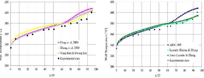
Fig. 12. Zhang et al. (2010) model Wall temperature distribution with

Fig. 12 shows the simulations of the wall temperature as a function of x/D obtained by using the four-equation model by Zhang et al. (2010). The best simulation is obtained with . The results are not surprising given that the model is designed for a constant turbulent Prandtl number equal to 0.9. However, is possible to obtain good results also by imposing .

a) b)

Fig. 13 Wall temperature distribution obtained by Deng et al. (2000) with different values of and

The simulations obtained with the model of Deng et al. (2000) (

Fig. 13) show that the predicted wall temperatures are very much influenced by the turbulent Prandtl number, though they are less influenced by (other cases in which the influence of is greater are reported below). In this case, the temperature peak decreases of about 36 °C and it still shows high overestimation of the experimental data. The results suggest further investigation in order to understand the capability of the different models.

(5)

45

a) b)

Fig. 14. Wall temperature distribution obtained by AKN (1995) with different values of and

Fig. 14 shows the results obtained with the model of AKN (1995). The best simulation, at least considering the location of the deterioration phenomenon along the pipe, is obtained with , but with respect to the simulation made with the Deng et al. model there is an increased recovery and an increase in the difference between the peaks for and

that is approximately equal to 95 °C.

More interesting results were obtained using the “hybrid model” Yang Shih + Hwang Lin (Fig. 15). This model exhibits the deterioration near the wall and the recovery. We started the series of simulations with high values of and as the trend of the experimental data is overestimated in these cases and we corrected them by gradually decreasing the values of these two parameters to the values and .

(6)

46

a) b) .

c)

Fig. 15. Wall temperature distribution obtained by Yang Shih + Hwang Lin. with different values of

In Fig. 15 c) the temperature peaks are almost coincident and the deterioration near the wall decreases. These results become very close to experimental data. On this basis, it is possible to consider other cases where different turbulent velocity field two-equation models are combined with turbulent thermal field models. Fig.16 shows the combination of Launder and Sharma (1974) model and Zhang et al. (2010) model.

(7)

47

a) b) .

c)

Fig.16 Wall temperature distribution obtained by LS+Zhang. with different values of

These models have obtained a reasonable result for the level of wall temperature; furthermore, the deterioration is not far from the experimental data but the recovery is now completely predicted. Both models are quite reactive to changes in both the considered values; specifically, decreasing leads to a decrease in the term of turbulent dissipation rate and an increase of turbulent kinetic energy, while decreasing , the wall temperature becomes closer to the experimental data because the temperature peak is delayed.

In (Fig.17, Fig. 18, Fig. 19) the distributions as a function of y+ of the production of turbulent kinetic energy due both the shearing and the buoyancy are shown all along the pipe for LS+Zhang model. It is possible to notice how the distribution changes with changing the considered parameters.

(8)

48

a) and b) and

Fig.17. Production of turbulence due to buoyancy obtained by LS+Zhang model

a) and b) and

Fig. 18. Production of turbulence due to shearing obtained by LS+Zhang model

a) and b) and

(9)

49

a) b)

c) d)

e)

Fig. 20. Wall temperature distribution obtained by LS+Deng model with different values of

In the previous cases (Fig. 20) these two changes in model parameters are tested, even though Launder and Sharma + Deng model is less reactive than the models shown above. Specifically, the Launder and Sharma + Deng model demonstrates that by changing the equations of thermal

(10)

50

fields, the result of the simulation are very different. This happens because the Zhang et al (2010) model is less reactive to deterioration and underestimates the wall temperature, while; on the contrary, in the Deng et al. (2000) model the temperature is overestimated.

Other simulations using Jones-Launder + Zhang models were performed. Fig. 21 shows that the sensitivity of the new hybrid model is still high. The recovery is better than for the LS+Zhang model. Finally, when decreasing the coefficient , both recovery and deterioration decrease.

a) b)

c) d)

Fig. 21 Wall temperature distribution obtained by JL+Zhang with with different values of

To sum up, the hybrid models are very sensitive to variations of both the turbulent Prandtl number and the coefficient. This means that, across the pseudocritical temperature, each model is “reactive” to deterioration. In these conditions, the decrease of the turbulent dissipation rate and the increase of the turbulent kinetic energy lead to a significant change of the simulation results. Therefore, only with a four-equation model it is possible to adjust the trend of the wall temperature. Other simulations were made also using the model, as shown in Fig. 22. This

(11)

51

model underestimates the wall temperature and it is therefore necessary to increase the coefficient accordingly, thus increasing the turbulent Prandtl number in order to decrease the turbulent heat diffusion in the flow, which makes the heat transfer less effective (Jaromin, 2012).

Fig. 22 Wilcox. Wall temperature distribution

Downward flow

Fig.23. and as default values in THEMAT

We observe in Fig.23 that for downward flow there are good results even for the default values and . As already observed, for a fluid close to pseudocritical conditions, the molecular Prandtl number is very much higher than unity. For instance, when the operating pressure is 23.5 MPa water reaches a value of greater than 14 at the peak. In order to investigate this effect, calculations were performed by implementing the following formulation for the turbulent Prandtl number as in Gräber (1970):

(12)

52

Fig. 24. and Gräber relation for Prt implemented in THEMAT

Fig. 24 shows that there is no significant difference between the results obtained with the default turbulent Prandtl number implemented in THEMAT code and those obtained when using the Gräber formulation. This result can be justified if we take into account that the region in which there is a strong variation of the molecular Prandtl number is concentrated over very short segment of the pipe.

It is worth noting that the results shown in Fig. 24 present a good trend, thus it is not necessary to reduce the turbulent Prandtl number as was instead needed in the case of upward flow to search for a better approximation. Hence, when considering the downward flow the buoyancy effect is not significant with respect to the upward flow case.

Nevertheless, some models do not work very well as the wall temperature crosses the pseudocritical temperature. Indeed, AKN (1995) and Deng et al. (2000) exhibit a very similar trend overestimating experimental data. On the contrary, the LS+Zhang model works better. Also Zhang et al.(2010) gives good results, this is hardly surprising given that this model is based on . As for the other three models, two of them are based on the Zhang model for the thermal field, they basically evolve following the experimental data.

(13)

53

4.1.2 Comparison between LES data and STAR CCM+

Case series 1: D = 6.28 mm, Tin = 300 °C, G = 509 kg/(m

2

s), q’’ = 420 kW/m

2

Upward flow

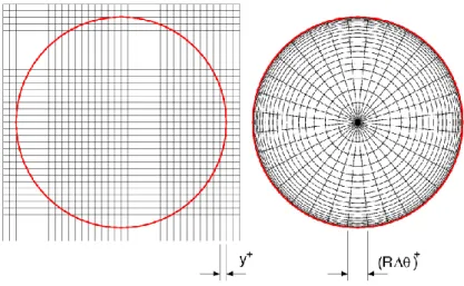
In this section, a new set of analysis based on LES data, available from the Swiss research centre Paul Scherrer Institut (PSI), is presented. These data have been already used by researchers at PSI to study the Pis’menny case because the computational domain is shorter with respect to other available cases. Furthermore the Reynolds number is lower (around 11200). The main difficulty when using the Pis'menny pipe for the available LES code was constituted by the non-Cartesian geometry. At first time, the experiment of Pis'menny was conducted in a tube with circular cross section ( Fig. 25) making use of different choices, but this led to computational problems. Finally, it was decided to consider a Cartesian domain with the same hydraulic diameter (6.28mm) (Fig. 26). This approach was based on the assumption that the phenomena that lead the heat transfer enhancement or deterioration at supercritical pressures are confined to the vicinity of the heated walls, and that the curvature of these walls plays a secondary role. This is confirmed in the work of Kim et al. (2007), where DHT has been studied experimentally in flow channels of circular and non-circular tube. The data showed very similar behaviour to the channel wall temperature circular and rectangular cross-section for the same boundary conditions.

Fig. 25. Possible approaches to cover cylindrical pipe with orthogonal grid: (a) using IBM method, (b) using cylindrical grid

(14)

54

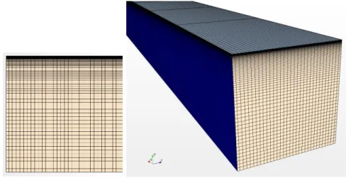
Fig. 26 Original problem domain (left) and the one considered in this work (right).

Thus, maintaining unchanged the other initial conditions, they have verified that in order to obtain comparable data with respect to the original case, it was necessary to increase the heat flux from 390 kW/m2 to 420 kW/m2. Specifically, they decided to increase the heat flux as the pipe has a larger surface area than the channel per unit volume of fluid. To perform numerical trials, they used two-equations only with SGDH. The experimental results from Pis’menny can be used for a reference comparison - without claiming they are exactly similar but very close to them, in order to make judgement about the quality of simulations (Fig. 27). The analyses were made for upward and downward flow. Fig. 27 shows that the model is very close to experimental data as concerned the distribution of the wall temperature for both upward and downward flow.

Fig. 27 Wall temperature distribution with q=420 kW/m2 calculated by LES

STAR CCM+ is used in this thesis to make a comparison with LES data. To this aim, we maintained the same channel geometry and the same inlet conditions, thus imposing a heat flux that is equal to 420 kW/m2. The computational domain is shown in Fig. 28. Specifically, on the

(15)

55

left side of Fig. 28, the inlet channel section is represented, while on the right side a three-dimensional representation of the channel is shown. On the top of the channel there is the wall, which is heated as in the experiment after 0.4 m from the inlet, in order to stabilise the flow before starting the heating process. The computational domain is characterised by the following dimensions:

 streamwise: x = 1000 mm;

 normal: y =3.14 mm;

 spanwise: z = 3.14 mm.

Fig. 28. Detailed view of the mesh adopted with STAR-CCM+ for the channel

We made the analyses on the three-dimensional geometry using volumetric meshes and a computational grid adapted from the one of Badiali (2011) for a cylindrical pipe; more specifically:

 base size: 0.1 mm;

 prism layer stretching: 1.07;

 prism layer thickness: 1.54 mm;

 number of prism layers: 55.

The value of y+ at the wall is always less than 0.5, as it is suggested for low-Reynolds number turbulence models.

In Fig. 29, Fig. 30, Fig. 31, Fig. 32 and Fig.33 it is possible to observe that the low-Reynolds models tend to overestimate, as usual, the wall temperature, while the model tends to underestimate the experimental data, without detecting the phenomena of deterioration and recovery. Specifically, from the simulation it is possible to observe that the wall temperature rapidly increases starting from x/D = 55, showing the usual peak when x/D is around 75. So,

(16)

56

with respect to the experimental data (x/D = 90), both the peak and the recovery phase occur before the experimental data.

However, the turbulent models can predict quite well the wall temperature in the normal heat transfer region (x/D < 55), while the model exhibits a good performance up to x/D = 60, even though it does not calculate properly the deterioration and the recovery. Finally, the temperature peak is delayed.

The temperature distribution in the region around the wall is very steep, thus creating strong buoyancy forces. In Fig. 29, Fig. 30 and Fig. 31 it is indeed possible to see a strong buoyancy effect that leads to expected M-shaped velocity profiles. When looking at Fig. 32 and Fig.33 it can be noted that the velocity profile becomes flatter with increasing the axial coordinate.

a) b)

Fig. 29. AKN model. a) Axial velocity. b) Wall temperature distribution with .

a) b)

Fig. 30. Lien –the model is implemented in STAR CCM+ with the name “Standard low- Reynolds model”. a) Axial

(17)

57

a) b)

Fig. 31. V2F . a) Axial velocity. b) Wall temperature distribution with

a) b)

Fig. 32. SST . a) Axial velocity. b) Wall temperature distribution with

a) b)

(18)

58

Downward flow

The same flow and heat flux conditions are then imposed for the downward flow (Fig.34, Fig.35, Fig. 36, Fig. 37 and Fig. 38). The operating conditions are close to the pseudo-critical temperature and the models show relatively good performances. The only one that does not match too closely the expected trend is V2F. It is remarkable to note that, as usual, these completely different results were obtained by just changing the direction of gravity in the flow domain, showing the dramatic effect that “aided” mixed convection may have in deteriorating heat transfer with respect to “opposed” mixed convection. Very evidently the adopted models are capable to recognise this trend, though the quantitative accuracy in upward flow is far from desirable.

Fig.34 AKN model. a) Axial velocity. b) Wall temperature distribution with .

Fig.35. Lien –the model is implemented in STAR CCM+ with the name “Standard low- Reynolds model”. a) Axial

(19)

59

Fig. 36. V2F . a) Axial velocity. b) Wall temperature distribution with

Fig. 37. SST . a) Axial velocity. b) Wall temperature distribution with

(20)

60

4.1.3 Case series 2: D = 6.28 mm, Tin = 17 °C, G = 428 kg/(m

2

s), Upward flow

In this section, each simulation is made with reference to a low inlet temperature. In none of the experiments the pseudo-critical temperature is achieved at the wall or in the bulk fluid. The heat flux is gradually increased while the other conditions are kept constant. It is interesting to analyse these cases in order to evaluate whether the results presented above are still valid.

The analyses made for q’’= 113 kW/m2, shows that most models result in an almost monotone trend of the wall temperature, except for LS+Zhang where there is a very short recovery phase in the inlet region of the pipe. The results obtained by applying AKN (1995), shown in Fig. 39 and Deng et al. (2000), shown in Fig.40, are quite good resulting where experimental data are very close to the simulations. They do not change significantly for either variation in model parameters. The results obtained are very similar to Pucciarelli (2013) simulations.

The combination JL+Zhang, Fig.41, is quite “reactive” to both the changes of turbulent Prandtl number and less to the buoyancy coefficient. This happens also for LS+Zhang Fig.42. So, it is possible to obtain at low inlet temperature some variation in the simulation results, but this is strictly influenced by the model.

The worst simulations are with Yang Shih + Hwang Lin, Fig.43, and Zhang et al (2010), Fig.44. They underestimate the wall temperature more than the others, but they capable to react to the input change for both components.

a) b)

(21)

61

a) b)

Fig.40: Wall temperature distribution obtained by Deng et al. (2000) for different and

a) b)

Fig.41: Wall temperature distribution obtained by JL+Zhang for different and

a) b)

(22)

62

a) b)

Fig.43: Wall temperature distribution obtained by Yang Shih + Hwang Lin for different and

a) b)

Fig.44:Wall temperature distribution obtained by Zhang et al (2010) for different and

For the case with q’’= 181 kW/m2, some variation with respect to the previous cases is obtained when changing the values of the model parameters. The results obtained by applying AKN (1995), shown in Fig.45 and Deng et al. (2000), shown in Fig.46, do not change significantly from each other. Hence for these two models the buoyancy effect is negligible. However, they are very close to the experimental data and, as in the case with q’’= 113 kW/m2, even though both models underestimate it when the bulk enthalpy is low. Zhang et al. (2010) and the other three hybrid models are reactive to both the change of turbulent Prandtl number and the buoyancy coefficient as it is shown below in Fig.47, Fig. 48,Fig.49 and Fig.50. All these models are influenced by the increase of the turbulent heat diffusion along the tube. Fig.47b), Fig. 48b) and Fig.49b) show that the decrease of is relevant in the end of the pipe. The result are quite

(23)

63

good for JL+Zhang model with and and for YS+HL for and

.

Fig.50 highlights that the Zhang et al. (2010) model is influenced by buoyancy effect and the heat transfer.

a) b)

Fig.45. Wall temperature distribution obtained by AKN (1995) for different and

a) b)

(24)

64

a) b)

Fig.47. Wall temperature distribution obtained by JL+Zhang for different and

a) b)

Fig. 48. Wall temperature distribution obtained by LS+Zhang for different and

a) b)

(25)

65

a) b)

Fig.50. Wall temperature distribution obtained by Zhang et al. (2010) for different and

The results for q’’= 277 kW/m2, have a different characteristic than in the previous case. Fig.51 and Fig.52 show that AKN (1995) and Deng et al. (2000) give similar results like the previous case. The trend still increases in a monotonic way. Moreover, the problem is that the recovery is not noticed. JL+Zhang model, Fig.53, has an advantage, compared to Deng et al. (2000), because it can simulate a short recovery. However, this recovery takes place earlier with respect to the experimental data. These models, as LS+Zhang Fig. 54, are very interesting, because they do not show the characteristic overestimation of wall temperature, as other models or its underestimate as models. These hybrid models allow sometimes the possibility to quite regulate the sensitivity through the model coefficient and the in order to achieve better agreement with the experimental data. The combination YS+HLFig.55

, shows a very similar trend to that of the other previous models.

The Zhang et al. (2010) model Fig. 56 is more reactive than the hybrid models. Its limitation is to always underestimate the data especially if the wall temperature does not exceed the pseudocritical one. In this case, the model parameter for buoyancy has an interesting influence. For the three models before (Fig.53, Fig. 54 and Fig.55) decreasing the simulations results leading lower predictions of the wall temperature. Instead, for Zhang et al. model, decreasing

the simulated trend of wall temperature moves the peak temperature upstream and the model begins to show a small recovery.

(26)

66

a) b)

Fig.51. Wall temperature distribution obtained by AKN (1995) for different and

a) b)

Fig.52. Wall temperature distribution obtained by Deng et al. (2000) for different and

a) b)

(27)

67

a) b)

Fig. 54. Wall temperature distribution obtained by LS+Zhang for different and

a) b)

Fig.55. Wall temperature distribution obtained by YS+HL for different and

a) b)

(28)

68

The results for q’’= 370 kW/m2, have further different characteristics. An apparent deterioration is presented for the AKN (1995) model as shown in Fig.57 for with Unexpectedly, this model present an early recovery. This is the only cases where the profile of temperature, for AKN (1995) model, that reproduce an apparent deterioration for an heat transfer at low inlet temperature (Tin = 17 °C).

Deng et al., (2000) model (Fig. 58) does not change, at both different values of turbulent Prandtl

number and . The hybrid models (Fig. 59 and Fig.60), underestimate the results and anticipate the recovery. This effect is not evident as for cases with crossing the pseudocritical temperature. Furthermore, at high inlet temperatures it was necessary to decrease both the turbulent Prandtl number and , while for low inlet temperature we should act in the opposite way in order to get better results.

The YS+HL model, Fig.61, does not show considerable changes by assuming different turbulent Prandtl number values, but it shows changes with different values of . For , Fig.61

b); in particular, it changes in a unexpected way after 300 kJ/kg showing a flat trend following the slope of the other two simulations.

The results from Zhang et al. model shown in Fig. 62 is the most reactive to model parameter changes. In this case, it is also evident that decreasing the peak in the simulation becomes

thinner and it still moves on towards the upstream.

a) b)

(29)

69

a) b)

Fig. 58 Wall temperature distribution obtained by Deng et al. (2000) for different and .

a) b)

Fig. 59. Wall temperature distribution obtained by JL+Zhang for different and .

a) b)

(30)

70

a) b)

Fig.61. Wall temperature distribution obtained by YS+HL for different and .

a) b)

Fig. 62. Wall temperature distribution obtained by Zhang et al (2010) for different and .

To summarise, at low inlet temperatures there is no specific model that can be considered as the best, but it was possible to highlight which models are sensitive to parameter changes. Only Deng et al. (2000) and AKN (1995) behave for predicting the heat transfer deterioration but the recovey of heat transfer is not predicted. All the other models, instead, underestimate the experimental data.

(31)

71

4.1.4 Case series 3: D = 6.28 mm, Tin = 200 °C, G = 249 kg/(m

2

s), Upward flow

Also the experiments considered in this section do not achieve the pseudo-critical temperature at the wall. The mass flux is still low, but the inlet fluid temperature is higher than in previous cases and it is possible to observe deterioration. The heat flux is gradually increased while the other conditions are kept constants. It is interesting to analyse these cases in order to evaluate whether the results obtained from the analysis of the other cases above are still valid.

As before, we started considering the case with a heat flux of 167 kW/m2. Initially, we evaluated each model with for different values of the turbulent Prandtl number. Then, we choose the best simulation for evaluating the importance of buoyancy generation through the coefficient

. Sometimes we tested this coefficient for two different values of the turbulent Prandtl

number.

Fig. 63 a) b)

Fig. 63 shows that AKN (1995) has become reactive to parameters changes and its trend is quite similar to the experimental data. The results obtained here are very different to the calculation made by Pucciarelli (2013), who adopted AHFM models with the parameters used by Kenjereš. AKN (1995) overestimates the experimental data and its best performance is with and

. Therefore it is important to decrease the buoyancy effect and again the peak of

temperature moves to the left. Nevertheless, AKN (1995) seems to be the best model for this case, Fig.64. The Deng model still has a similar trend with respect to the one of the AKN model. JL+Zhang, Fig. 65a), shows significant variation of the wall temperature changing the turbulent Prandtl number, and the first temperature peak moves from x/D=45 to x/D=50. We also made the simulation for Fig. 65b). LS+Zhang Fig. 66a) has a similar trend with respect to the previous model. The simulations calculate the peak temperature earlier at x/D=44.5. In Fig. 67, the YS+HL model shows a flat trend decreasing and a peak appears with changing . In Fig.68 Zhang et al. model (2010) fails in predicting the main phenomena as YS+HL.

(32)

72

a) b)

Fig. 63. . Wall temperature distribution obtained by AKN (1995) for different and .

a) b)

Fig.64 . Wall temperature distribution obtained by Deng et al (2000) for different and .

a) b)

(33)

73

a) b)

Fig. 66. Wall temperature distribution obtained by LS+Zhang for different and .

a) b)

Fig. 67. . Wall temperature distribution obtained by YS+HL for different and .

a) b)

(34)

74

The results for q” = 253 kW/m2 show again deterioration. Now the experimental data of wall temperature are quite close to the pseudocritical value. Also in these models cases it is possible to observe the modification made changing the two model parameters; Fig.69 and Fig.70 present the simulation made with AKN (1995) and Deng et al. models (2000). As usual, all simulations overestimate the experimental data, except for Zhang et al. (2010), but they catch the overall trend. It is important to notice that the recovery phase occurs later for AKN (1995) and Deng et al. (2000), but with JL+Zhang (Fig.71), LS+Zhang (Fig.72) and YS+HL (Fig.73) it starts at x/D=30 as in the experimental data. In Fig. 74, the Zhang et al. (2010) model once again underestimates the peaks in the wall temperature, but it is the best when getting closer to pseudocritical condition.

a) b)

Fig.69 . Wall temperature distribution obtained by AKN (1995) for different and .

a) b)

(35)

75

a) b)

Fig.71. Wall temperature distribution obtained by JL+Zhang for different and .

a) b)

Fig.72 . Wall temperature distribution obtained by LS+Zhang for different and .

a) b)

(36)

76

a) b)

Fig. 74. . Wall temperature distribution obtained by Zhang et al (2010) for different and .

The results for q’’= 289 kW/m2, have similar characteristics to the previous case. Now the experimental data of wall temperature cross the pseudocritical value. All the models, except for Zhang et al. (2010), overestimate the experimental data and show an early recovery phase (Fig.75, Fig 76, Fig.77, Fig.78, Fig.79 and Fig.80) it is shown that the Zhang et al. (2010) underestimates the peak in wall temperature but it is still the best when getting closer to the pseudocritical condition.

a) b)

(37)

77

a) b)

Fig 76 Wall temperature distribution obtained by Deng et al. (2000)for different and .

a) b)

Fig.77 Wall temperature distribution obtained by JL+Zhang for different and .

a) b)

(38)

78

a) b)

Fig.79 Wall temperature distribution obtained by YS+HL for different and .

a) b)

Fig.80 Wall temperature distribution obtained by Zhang et al. (2010) for different and .

4.1.5 Case series 4: D = 9.5 mm, T

in

= 100 °C, G = 248 kg/(m

2

s), Upward flow

The experiments considered in this section are characterised by a lower inlet temperature if compared with previous ones and by a larger tube diameter. Greater buoyancy effects are present, especially at high heat flux; this is obviously due to the larger internal diameter.

The first case is characterised by a low heat flux q’’=118 kW/m2, (Fig.81, Fig.82, Fig.83, Fig.84 and Fig. 85). Unfortunately, the YS+HL did not converge for this analysis and its results cannot be therefore presented.

(39)

79 *

a) C_ε3=1 b) 〖Pr〗_t=0.9

Fig.81 Wall temperature distribution obtained by AKN (1995) for different and .

a) b)

Fig.82 Wall temperature distribution obtained by Deng et al. (2000) for different and .

a) b)

(40)

80

a) b)

Fig.84 Wall temperature distribution obtained by LS+Zhang for different and .

a) b)

Fig. 85. Wall temperature distribution obtained by Zhang et al. (2010) for different and .

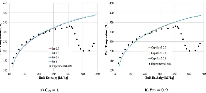
The second case has a lower heat flux q’’=175 kW/m2

. In Pucciarelli’s work (2013) the recovery phase became early for AKN (1995) and Deng et al. (2000). Now these models give better results, Fig.86 and Fig.87. Also for the other models it is possible to obtain good results (Fig. 88, Fig. 89 and Fig.90) except for Zhang et al. (2010) Fig 91.

(41)

81

a) b)

(42)

82

a) b)

Fig. 89 Wall temperature distribution obtained by LS+Zhang for different and .

a) b)

(43)

83

The third upward flow case is with heat flux q’’=275 kW/m2

. Unfortunately YS+HL did not converge for this simulation. In this case, the models are less reactive, in particular when the turbulent Prandtl number changes. The results are anyway always good especially for AKN (1995) Fig. 92 and Deng et al. (2000) Fig.93. For these two models the recovery phase starts nearly at 550 kJ/kg. Changing there are a variations only in the recovery phase and not

before the peak temperature (Fig. 92, Fig.93, Fig. 94, Fig. 95 and Fig. 96).

a) b)

Fig. 92 Wall temperature distribution obtained by AKN (1995) for different and .

a) b)

(44)

84

a) b)

Fig. 94 Wall temperature distribution obtained by JL+Zhang for different and .

a) b)

(45)

85

The fourth upward flow case is with a heat flux q’’=396 kW/m2

. Unfortunately, YS+HL did not converge again. In this case, the models are again less reactive, in particular when the turbulent

Prandtl number changes. The results are good especially for AKN (1995) (

Fig 97) and Deng et al. (2000) (Fig.98). Also Zhang et al. (2010) (Fig. 101) gives good results, though it still underestimates the experimental data. The other results are showed in Fig. 99 and Fig. 100.

.

a) b)

Fig 97. Wall temperature distribution obtained by AKN (1995) for different and .

a) b)

(46)

86

a) b)

(47)

87

The last considered case is with a heat flux of q’’=495 kW/m2

. Unfortunately, the AKN (1995), Deng et al. (2000) and YS+HL did not converge again. The other models (Fig. 102 and Fig. 103) can predict reasonably the trend until the first recovery and then show flat temperature profiles with respect to the experimental data. Zhang et al. (2010) (Fig. 104) shows the effect of an increase in buoyancy; this model reproduces quite reasonably the trend, though underestimating the experimental data.

a) b)

(48)

88

a) b)

(49)

89

4.2 Experimental data by Ornatskii et al. (1971)

These experiments involve supercritical water at 25.5 MPa in a vertical tube for upward flow direction. The Authors used a small internal diameter (3 mm) and the operating conditions are far from the pseudocritical temperature. They adopted a very high mass flow rate (1500 kg/sm2), this brings a buoyancy effect less important. The deterioration of heat transfer is due to strong variation in fluid density along the pipe axis and not only near the wall. This occurs because the bulk fluid temperature exceeds the pseudocritical value and then there is a strong fluid acceleration.

The inlet fluid temperature is low (Tin= 300 K) and the heat fluxes are relatively large (q”=1320

kW/m2 and 1810 kW/m2).

The nodalization is the same as in previous studies (Pucciarelli, 2013) and does not include heat conduction within the wall; the axial dimension of the cell is uniform while the radial dimension is varied by a geometrical progression (Ratio = 1/1.08). This allows obtaining a value for y+ that is lower than 0.5 for the first node near the wall.

The parameters of the nodalization for the experimental data used for Ornatskii et al. (1971) are as follows:

4.2.1 Case series 1: D = 3 mm, T

in

= 300 K, G = 1500 kg/(m

2

s),

q’’ = 1320 kW/m

2

Upward flow

It is interesting to note that in the experimental data trend, the deterioration occurs earlier than the pseudo-critical temperature is reached, while in the calculations it occurs when it is crossed. All models show good performances before the deterioration, when the slope of the wall temperature is linear. AKN (1995), Deng et al. (2000) and YS+HL(Fig.105, Fig.106 and Fig. 109) provide similar trends and they underestimate the experimental data. JL+Zhang model and LS+Zhang model (Fig.107 and Fig. 108) are the worst with wall temperatures exceeding 1000 °C and then a recovery phase appears that it is not present in the experimental data. For and ( Fig.107b)) it is possible to obtain an improvement of predictions for the deterioration phenomenon with the JL+ Zhang model. Zhang et al. (2010) (Fig. 110) shows anyway the best performance, though with the usual delay in deterioration.

(50)

90

a) b)

(51)

91

a) b)

Fig. 109 Wall temperature distribution obtained by YS+HL for different and .

a) b)

(52)

92

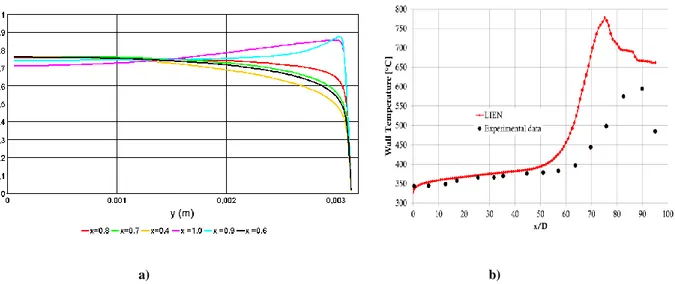
Fig. 111 shows the axial velocity radial trends calculated at different pipe cross sections with the Zhang et al. (2010) model. It is possible to note that the velocity maintains a similar radial profile all along the pipe length. The mass flux is large enough, so that the buoyancy effect is negligible. Furthermore, the laminarization is not the mechanism leading to deterioration

Fig. 111 Axial velocity radial trends

4.2.2 Case series 2: D = 3 mm, T

in

= 300 K, G = 1500 kg/(m

2

s),

q’’ = 1810 kW/m

2

Upward flow

At high turbulent Prandtl number all models fail the prediction of the deterioration phenomenon. All models try to reproduce the deterioration and recovery phase but the peak of temperature is much higher than in the experiment, up to 1000 °C (Fig.112, Fig. 113, Fig. 114, Fig. 115, Fig.116 and Fig. 117). Decreasing turbulent Prandtl number, is possible to notice that the AKN (1995), Deng et al. (2000) and YS+HL models, predict the peak of temperature closer to the experiment (Fig.112a), Fig. 113a) and Fig.116 a)). All models show a good trend before the deterioration phase when the slope of the wall temperature increases.

(53)

93

a) b)

Fig. 113 Wall temperature distribution obtained by Deng et al. (2000) for different and .

a) b)

(54)

94

a) b)

(55)

95

In the above figures, whenever the temperature shows discontinuities after reaching too high values this is interpreted as absence of information from the property package for this temperature range.

Fig.118 shows that, also in this case, the axial velocity distribution does not show buoyancy effects all along the pipe length. The absence of buoyancy, in fact, is confirmed in the velocity profiles at various axial locations by the absence of the classical M-shape that characterises mixed convection. This suggests that the laminarization is not the principal mechanism of deterioration. Most probably the deterioration is due to the strong acceleration; in fact, the turbulent kinetic energy (Fig. 119) increases considerably in the presence of a strong acceleration along the pipe. The wall fluid temperature passes through the pseudocritical value generating a local transition from liquid-like to gas-like fluid.

Fig.118 Axial velocity trends

(56)

96

4.3 Experimental data by Watts (1980)

These experiments are made for supercritical water at 25 MPa (Tpc=384.9°C) in a vertical tube

for upward direction with an internal diameter of 25.4 mm. It is here considered only a set of data with nominal inlet temperature kept constant at 150 °C and the operating conditions varying for both the heat and the mass fluxes. Table 5 summarizes the boundary conditions considered in the present work.

Tin [°C] G [kg/(m2s)] q’’ [kW/m2] D_in [mm]

150 273 250 25.4 Upward

150 367 250 25.4 Upward

150 526 250 25.4 Upward

Table 5: Operating conditions considered in the present work for the data by Watts (1980)

The nodalization is the same as in previous studies (Pucciarelli, 2013). The parameters of the nodalization for the experimental data used for Watts et al. (1980) are as follows:

4.3.1 Case series 1: D = 25.4 mm, T

in

= 150 °C, q’’ = 250 kW/m

2

Upward flow

The experiments considered in this section are characterised by relatively low inlet temperature and high mass flux. The wall and bulk temperatures are more or less close to the pseudo-critical temperature; anyway wall temperature always remains below this threshold. In the set of experiments, the mass flux is gradually increased while the other conditions are kept constant. Looking at the experimental data trends, the effect of increasing the mass flux is clearly that the peak in wall temperature is progressively postponed, becomes weaker and eventually disappears. The results obtained for the case with G= 273 kg/(m2s) are presented below. Applying AKN (1995), whose results are shown in Fig. 120 and Deng et al. (2000), Fig. 121, the temperature trend in the recovery phase is overestimated. The other four models instead underestimate the

(57)

97

experimental data (Fig. 122, Fig. 123, Fig. 124 and Fig. 125). All models reproduce anyway qualitatively the trends of the experimental data.

a) b)

(58)

98

a) b)

(59)

99

a) b)

Fig. 125. Wall temperature distribution obtained by Zhang et al., (2010) for different and .

Fig. 126 shows the axial velocity profile calculated with the AKN (1995) model with for the case with and . The pseudo-critical temperature is not crossed along the pipe and the

deterioration is once again due to laminarization.

Fig. 126 Axial velocity trends

The results for G = 367 kg/(m2s) show again deterioration. Unfortunately the combination YS+HL did not converge and its results are not displayed. For the other models, it is possible to observe the modification made changing the two parameters. All the simulations underestimate the experimental data of wall temperature (Fig. 127, Fig. 128, Fig.129, Fig. 130 and Fig. 131). It is important to notice that the recovery phase for all models, but not for Deng et al., (2000), starts quite at the same x/D of the experimental data when =1 at .

(60)

100

a) b)

Fig. 128 Wall temperature distribution obtained by Deng et al., (2000) for different and .

a) b)

(61)

101

a) b)

Fig. 131 Wall temperature distribution obtained by Zhang et al., (2010) for different and .

The case discussed below is characterized by high mass fluxes; the pseudo-critical temperature is still not crossed by the wall temperature, and the recovery phase occurs at the end of the pipe. Unfortunately the calculations with the model of Deng et al., (2000) did not converge. All the other simulation present rather good results (Fig. 132, Fig. 133, Fig. 134 and Fig. 135) except for Zhang et al., (2010) model, where all the obtained wall temperature trend overestimates the experimental data (Fig. 136). Anyway Zhang et al., (2010) model is the only that can reproduce the peak of temperature.

(62)

102

a) b)

(63)

103

a) b)

Fig. 135 Wall temperature distribution obtained by YS+HL for different and .

a) b)

Fig. 136 Wall temperature distribution obtained by Zhang et al., (2010) for different and .

In this case no deterioration is predicted. The buoyancy effects are negligible in this case; in fact, it is possible to observe that in the radial profile of axial velocity (Fig. 137), they are more limited.

(64)

104