59. τ Branching Fractions
Revised August 2017 by S. Banerjee (University of Louisville), K. Hayes (Hillsdale College), A. Lusiani (Scuola Normale Superiore and INFN, sezione di Pisa)
In order to make optimal use of the experimental data to determine the τ branching fractions, their uncertainties, and their correlations, we perform a global minimum χ2 fit using the measured values, their uncertainties, their statistical correlations, their dependencies on external parameters and common systematics, and the relations that hold between the branching fractions, including a unitarity constraint on the sum of all the exclusive τ decay branching fractions. Starting with this edition, we use a new fit procedure, which has been elaborated by the Tau Physics Group within the Heavy Flavour Averaging Group (HFLAV) [1].
In the following, we use “branching fraction” to refer to the partial decay fraction of a particle like the τ into a specific decay mode, and “branching ratio” to refer to quantities derived from the branching fractions [2], like for instance a ratio of two branching fractions, or a ratio of two linear combinations of branching fractions.
This review contains only minor revisions with respect to the 2016 edition.
59.1. The constrained fit to τ branching fractions
The τ Listings contains 242 τ decay modes, out of which 61 are Lepton Family number, Lepton number, or Baryon number violating modes. The fit computes the branching fractions of 112 decay modes. Although no new τ branching fraction and ratio measurements have been released since the 2015 edition, the fit in this edition includes more experimental measurements (169, up from 143 in 2015) and determines in the fit several additional τ branching fractions and ratios, relying on a larger and updated set of constraints that relate the branching fractions and ratios between themselves. The measurements are treated as follows [1].
Many published measurements depend on external parameters such as the τ pair production cross-section in e+e− annihilations at the Υ(4S) peak. We compute the size and sign of these dependencies and update the measurements and their uncertainties to the current values of the external parameters. The dependencies on common systematic effects are also determined in size and sign, and all the common systematic dependencies of different measurements are used together with the published statistical and systematic uncertainties and correlations in order to compute a single all-inclusive variance and covariance matrix of the experimental measurements. All the measurements, their uncertainties, and their correlations were taken from the respective published papers. Their values and the constraints used in the fit are reported in the τ Listings section that follows this review. If only a few measurements are correlated, the correlation coefficients are listed in the footnote for each measurement (see for example Γ(particle− ≥ 0 neutrals ≥ 0 K0ν
τ (“1-prong”))/Γtotal). If a large number of measurements are correlated, then the full correlation matrix is listed in the footnote to the measurement that first appears in the τ Listings. Footnotes to the other measurements refer to the first measurement. For example, the large correlation matrices for the branching fraction or ratio measurements contained in Refs. [3,4] are listed in Footnotes to the Γ(e−νeντ)/Γ
total and Γ(h−ντ)/Γtotal measurements respectively. M. Tanabashi et al. (Particle Data Group), Phys. Rev. D 98, 030001 (2018)
The constraints between the τ branching fractions and ratios include coefficients that correspond to physical quantities, like for instance the branching fractions of the η and ω mesons. All quantities are taken from the 2015 edition of the Review of Particle Physics. Their uncertainties are neglected in the fit.
Compared to the 2015 edition, the fit now includes several additional modes, mainly related to the most recent BaBar papers on high multiplicity modes [5] and KS0KS0 modes [6] and the Belle paper on neutral kaon modes [7]:
B(τ → π−π0K0 SKS0ντ) B(τ → K−K−K+ν τ) B(τ → K−π0ην τ) B(τ → π−K¯0ην τ) ;
Also, the following components of τ -decay modes are now included [5,8,9]: B(τ → π−2π0ην τ (η → π+π−π0) (ex. K0)) B(τ → 2π−π+ην τ (η → π+π−π0) (ex. K0)) B(τ → 2π−π+ην τ (η → γγ) (ex. K0)) B(τ → π−2π0ων τ (ex. K0)) B(τ → 2π−π+ων τ (ex. K0)) B(τ → π−f1ντ (f1 →2π−2π+)) . B(τ → K−φντ) .
We obtain the branching fraction of τ → a−
1(→ π−γ)ντ using the ALEPH estimate for B(a−
1 → π−γ) [3], which uses the measurement of Γ(a−1 → π−γ) [10]. In the fit, we assume that B(τ− → a−
1ντ) is equal to B(τ → π−π−π+ντ (ex. K0, ω)) + B(τ → π−2π0ν
τ (ex. K0)).
In some cases, constraints describe approximate relations that nevertheless hold within the present experimental precision. For instance, the constraint B(τ → K−K−K+ν
τ) = B(τ → K−φντ) × B(φ → K+K−) is justified within the current experimental evidence.
In the fit, scale factors are applied to the published uncertainties of measurements only if significant inconsistency between different measurements remain after accounting for all relevant uncertainties and correlations. After examining the data and the fit pulls, it has been decided to apply just one scale factor of 5.4 on the measurements of B(τ → K−K−K+ν
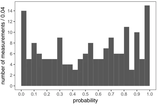
τ). The scale factor has been computed and applied according to the standard PDG procedure. Without the scale factor applied, the χ2 probability of the fit is about 2%. On a per-measurement basis, the pull distribution in figure 59.1 indicates that just a few measurements have more than 3σ pulls. (The uncertainties to obtain the pulls are computed using the measurements variance matrix and the variance matrix of the result, accounting for the fact that the variance matrix of the result is obtained from the measurement variance with the fit.) The pull probability distribution in figure 59.2 is reasonably flat. With many measurements some entries on the tails of the normal distribution must be expected. There are 169 pulls, one per measurement. They are partially correlated, and the effective number of independent pulls is equal to the number
0 2 4 6 8 10 12 14 16 18 20 −6 −5 −4 −3 −2 −1 0 1 2 3 4 5 6 pull n umber of measurements / 0.24
Figure 59.1: Pulls of individual measurements against the respective fitted quantity. No scale factor is used.
0 2 4 6 8 10 12 14 0.0 0.1 0.2 0.3 0.4 0.5 0.6 0.7 0.8 0.9 1.0 probability n umber of measurements / 0.04
Figure 59.2: Probability of individual measurement pulls against the respective fitted quantity. No scale factor is used.
of degrees of freedom of the fit, 124. Only the τ → K−K−K+ν
τ decay mode has a pull that is inconsistent at the level of more than 3σ even if considered as the largest pull in a set of 124. This confirms the choice of adopting just that one scale factor.
After scaling the error the 2016 constrained fit has a χ of 134.9 for 124 degrees of freedom, corresponding to a χ2 probability of 24%. We use 169 measurements and 84 constraints on the branching fractions and ratios to determine 129 quantities, consisting of 112 branching fractions and 17 branching ratios. A total of 85 quantities have at least one measurement in the fit. The constraints include the unitarity constraint on the sum of all the exclusive τ decay modes, Ball = 1. If the unitarity constraint is released, the fit result for Ball is consistent with unitarity with 1 − Ball = (0.07 ± 0.10)%.
For the convenience of summarizing the fit results, we list in the following the values and uncertainties for a set of 46 “basis” decay modes, from which all remaining branching fractions and ratios can be obtained using the constraints. Unlike in previous editions, the basis decay modes are not intended to sum up to 1. The new unitarity constraint corresponds to a linear combination of the basis modes weighted by the coefficients listed in the following. The corresponding correlation matrix is listed in the τ Listings.
decay mode fit result (%) coefficient
µ−¯νµντ 17.3936 ± 0.0384 1.0000 e−ν¯eντ 17.8174 ± 0.0399 1.0000 π−ντ 10.8165 ± 0.0512 1.0000 K−ντ 0.6964 ± 0.0096 1.0000 π−π0ν τ 25.4940 ± 0.0893 1.0000 K−π0ν τ 0.4329 ± 0.0148 1.0000 π−2π0ν τ (ex. K0) 9.2595 ± 0.0964 1.0021 K−2π0ν τ (ex. K0) 0.0648 ± 0.0218 1.0000 π−3π0ν τ (ex. K0) 1.0428 ± 0.0707 1.0000 K−3π0ν τ (ex. K0, η) 0.0478 ± 0.0212 1.0000 h−4π0ν τ (ex. K0, η) 0.1119 ± 0.0391 1.0000 π−K¯0ν τ 0.8395 ± 0.0140 1.0000 K−K0ν τ 0.1479 ± 0.0053 1.0000 π−K¯0π0ν τ 0.3821 ± 0.0129 1.0000 K−π0K0ν τ 0.1503 ± 0.0071 1.0000 π−K¯0π0π0ν τ (ex. K0) 0.0263 ± 0.0226 1.0000 π−K0 SKS0ντ 0.0233 ± 0.0007 2.0000 π−K0 SKL0ντ 0.1080 ± 0.0241 1.0000 π−π0K0 SKS0ντ 0.0018 ± 0.0002 2.0000 π−π0K0 SKL0ντ 0.0325 ± 0.0119 1.0000 ¯ K0h−h−h+ν τ 0.0247 ± 0.0199 1.0000 π−π−π+ν τ (ex. K0, ω) 8.9870 ± 0.0514 1.0021 π−π−π+π0ν τ (ex. K0, ω) 2.7404 ± 0.0710 1.0000 h−h−h+2π0ν τ (ex. K0, ω, η) 0.0980 ± 0.0356 1.0000 π−K−K+ν τ 0.1435 ± 0.0027 1.0000 π−K−K+π0ν τ 0.0061 ± 0.0018 1.0000 π−π0ην τ 0.1389 ± 0.0072 1.0000 K−ηντ 0.0155 ± 0.0008 1.0000
K−π0ην τ 0.0048 ± 0.0012 1.0000 π−K¯0ην τ 0.0094 ± 0.0015 1.0000 π−π+π−ηντ (ex. K0) 0.0219 ± 0.0013 1.0000 K−ωντ 0.0410 ± 0.0092 1.0000 h−π0ων τ 0.4085 ± 0.0419 1.0000 K−φντ 0.0044 ± 0.0016 0.8310 π−ωντ 1.9494 ± 0.0645 1.0000 K−π−π+ν τ (ex. K0, ω) 0.2927 ± 0.0068 1.0000 K−π−π+π0ν τ (ex. K0, ω, η) 0.0394 ± 0.0142 1.0000 π−2π0ων τ (ex. K0) 0.0071 ± 0.0016 1.0000 2π−π+3π0ν τ (ex. K0, η, ω, f1) 0.0014 ± 0.0027 1.0000 3π−2π+ν τ (ex. K0, ω, f1) 0.0769 ± 0.0030 1.0000 K−2π−2π+ν τ (ex. K0) 0.0001 ± 0.0001 1.0000 2π−π+ων τ (ex. K0) 0.0084 ± 0.0006 1.0000 3π−2π+π0ν τ (ex. K0, η, ω, f1) 0.0038 ± 0.0009 1.0000 K−2π−2π+π0ν τ (ex. K0) 0.0001 ± 0.0001 1.0000 π−f 1ντ (f1→2π−2π+) 0.0052 ± 0.0004 1.0000 π−2π0ην τ 0.0194 ± 0.0038 1.0000
Applying the fit procedure on the PDG 2015 inputs, the fit results differ from the 2015 fit by at most 20% of their uncertainty, for fitted quantities that have measurements with asymmetric errors, and by at most 5% of their uncertainty for the other quantities. The differences originate from the different treatment of asymmetric errors. The present fit procedure symmetrizes the errors as σsymm2 = (σ+2 + σ−2)/2, while the PDG 2015 fit did model the asymmetric error distributions in the fit. Comparing the results of the previous edition with the current fit, there are differences up to 2.3 times the fitted quantity uncertainty (2.3σ) for quantities that have no measurement included in the fit and are derived through the constraints. Those differences arise mainly from three changes: the unitarity constraint has been updated to accomodate several additional decay modes, the definitions of the respective quantities have been updated to use the additional decay modes, and the parameters of all constraints (typically, K, η, ω branching fractions) have been updated to the values reported in the last published PDG edition. For quantities that have measurements in the fit, the fitted values changed at most by 1.1σ, reflecting the inclusion of several additional measurements, especially on high-multiplicity decay modes. The uncertainties on the fit results are generally smaller than in 2015 because only one error scale factor is used and some additional measurements have been used.
In defining the fit constraints and in selecting the modes that sum up to one we made some assumptions and choices. We assume that some channels, like τ− → π−K+π− ≥ 0π0ν
τ and τ− → π+K−K− ≥ 0π0ντ , have negligible branching fractions as expected from the Standard Model, even if the experimental limits for these branching fractions are not very stringent. The 95% confidence level upper limits are B(τ−→ π−K+π− ≥0π0ν
τ) < 0.25% and B(τ− →π+K−K− ≥0π0ντ) < 0.09%, values not so different from measured branching fractions for allowed 3-prong modes containing charged kaons. For decays to final states containing one neutral kaon we assume that the
branching fraction with the KL are the same as the corresponding one with a KS. On decays with two neutral kaons we assume that the branching fractions with KL0KL0 are the same as the ones with KS0KS0.
59.2. BaBar and Belle measure on average lower branching
fractions and ratios
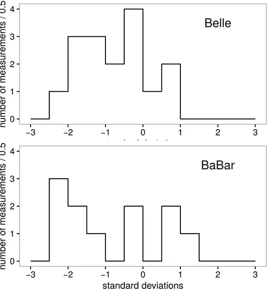
We compare the BaBar and Belle measurements with the results of a fit where all their measurements have been excluded. We find that that BaBar and Belle tend to measure lower τ branching fractions and ratios than the other experiments. Figure 59.3 shows histograms of the 27 normalized differences between the B-factory measurements and the respective non-B-factory fit results. The normalization is the uncertainty on the difference. The average normalized difference between the two sets of measurements is -0.8σ (-0.8σ for the 16 Belle measurements and -0.9σ for the 11 BaBar measurements).
59.3. Overconsistency of Leptonic Branching Fraction
Measure-ments
As observed in the previous editions of this review, measurements of the leptonic branching fractions are more consistent with each other than expected from the quoted errors on the individual measurements. When fitting just a single branching fraction using just its direct measurements, the χ2 per number of degrees of freedom is 0.31/4 for Be and 0.038/4 for Bµ. Assuming normal errors, the probability of a smaller χ2 is 1.1% for Be and 0.20% for Bµ.
59.4. Technical implementation of the fit
The fit computes a set of quantities denoted with qi by minimizing a χ2 while respecting a series of equality constraints on the qi. The χ2 is computed using the measurements mi and their covariance matrix Eij as χ2= (mi−Aikqk)tEij−1(mj−Ajlql) where the model matrix Aij is used to get the vector of the predicted measurements m′i from the vector of the fit parameters qj as m′i = Aijqj. In this particular implementation the measurements are grouped by the quantity that they measure, and all quantities with at least one measurement correspond to a fit parameter. Therefore, the matrix Aij has one row per measurement mi and one column per fitted quantity qj, with unity coefficients for the rows and column that identify a measurement mi of the quantity qj, respectively. The constraints are equations involving the fit parameters. The fit does not impose limitations on the functional form of the constraints. In summary, the fit requires: min(mi−Aikqk)tEij−1(mj −Ajlql), (59.1a)
subjected to fr(qs) − cr = 0, (59.1b)
where the left term of Eq. (59.1b) defines the constraint expressions. Using the method of Lagrange multipliers, a set of equations is obtained by taking the derivatives with respect
Belle
0 1 2 3 4 −3 −2 −1 0 1 2 3 standard deviations n umber of measurements / 0.5BaBar
0 1 2 3 4 −3 −2 −1 0 1 2 3 standard deviations n umber of measurements / 0.5Figure 59.3: Distribution of the normalized difference between the 27 B-factory measurements and non-B-factory measurements. The list includes 16 measurements of branching fractions and ratios published by the Belle collaboration and 11 by the BaBar collaboration that are used in the fit and for which non-B-factory measurements exist.
to the fitted quantities qk and the Lagrange multipliers λr of the sum of the χ2 and the constraint expressions multiplied by the Lagrange multipliers λr, one for each constraint:
minh(Aikqk−mi)tEij−1(Ajlql−mj) + 2λr(fr(qs) − cr) i
(59.2a)
(∂/∂qk, ∂/∂λr)[expression above] = 0 (59.2b)
Eq. (59.2b) defines a set of equations for the vector of the unknowns (qk, λr), some of which may be non-linear, in case of non-linear constraints. An iterative minimization procedure approximates at each step the non-linear constraint expressions by their first
order Taylor expansion around the current values of the fitted quantities, ¯qs: fr(qs) − cr = fr(¯qs) + ∂fr(qs) ∂qs ¯ ¯ ¯ ¯ ¯ qs (qs−q¯s) − cr, (59.3a) which can be written as
Brsqs−c′r, (59.3b)
where c′
r are the resulting constant known terms, independent of qs at first order. After linearization, the differentiation by qk and λr is trivial and leads to a set of linear equations
AtkiEij−1Ajlql+ Bkrt λr = AtkiEij−1mj (59.4a)
Brsqs = c′r, (59.4b)
which can be expressed as:
Fijuj = vi (59.5)
where uj = (qk, λr) and vi is the vector of the known constant terms running over the index k and then r in the right terms of Eq. (59.4a) and Eq. (59.4b), respectively. Solving the equation set in Eq. (59.5) by matrix inversion gives the the fitted quantities and their variance and covariance matrix, using the measurements and their variance and covariance matrix. The fit procedure starts by computing the linear approximation of the non-linear constraint expressions around the quantities seed values. With an iterative procedure, the unknowns are updated at each step by solving the equations and the equations are then linearized around the updated values, until the variation of the fitted unknowns is reduced below a numerically small threshold.
References:
1. D. Asner et al. (HFLAV), arXiv:1010.1589; Y. Amhis et al. (HFLAV), arXiv:1412.7515.
2. See the Introduction section of this edition of the Review of Particle Physics. 3. S. Schael et al. (ALEPH Collab.), Phys. Reports 421, 191 (2005).
4. J. Abdallah et al. (DELPHI Collab.), Eur. Phys. J. C46, 1 (2006).
5. J.P. Lees et al. (BABAR Collab.), Phys. Rev. D86, 092010 (2012), [arXiv:1209.2734]. 6. J.P. Lees et al. (BABAR Collab.), Phys. Rev. D86, 092013 (2012), [arXiv:1208.0376]. 7. S. Ryu et al. (BELLE Collab.), Phys. Rev. D89, 072009 (2014).
8. B. Aubert et al. (BABAR Collab.), Phys. Rev. Lett. 100, 011801 (2008). 9. K. Inami et al. (BELLE Collab.), Phys. Lett. B643, 5 (2006).