4 ANALYSIS OF LIFUS EXPERIMENTS 4.1 Introduction

(1)

87

4 ANALYSIS OF LIFUS EXPERIMENTS

4.1 Introduction

In the frame of the European Research Program aiming at developing GEN IV reactors and ADS systems, ENEA has been strongly involved in the experimental activities focused on the interaction between HLM and water. This kind of interaction may occur because of the rupture of one tube (or more) of the steam generator placed in XT-ADS [1]or ELSY [2-4] reactors’ pool.

Aiming at studying in depth and analysing physical phenomena and possible consequences of LBE-water interactions under a wide range of operating conditions, two experimental campaigns, one in the frame of DEMETRA domain of the IP-EUROTRANS Project [5], concerning studies on the XT-ADS, and one in the frame of ELSY Program [2], have been performed on the LIFUS 5 facility. It was designed. built and placed in ENEA Brasimone Research Center and was previously used in the past in order to investigate the Pb17Li-water interaction in the frame of the European Fusion Technology program[6,7].

In parallel with the ENEA experimental activities, a simulation activity of pre and post test analysis concerning the two campaigns has been carried out with SIMMER III code by the University of Pisa.

A detailed description of this activity and the main findings are described in this chapter.

4.2 Experimental activity

LIFUS 5 facility was designed in ENEA Brasimone in order to investigate the phenomenology of the interaction between heavy liquid metals, in particular lead and lead alloys, and water under several operating conditions such as water pressure up to 20 MPa and initial liquid metal temperature up to 500 °C [1]. Six tests have been carried out. Four tests belonged to the IP-EUROTRANS Project, while the other related to the ELSY program.

The facility was modified several times, according to the test conditions. Therefore, a summary of the several facility configurations used in the overall campaign will be given in the following paragraphs, starting from the original one up to the latest one.

4.2.1 Original configuration of the facility and Test n.1 conditions

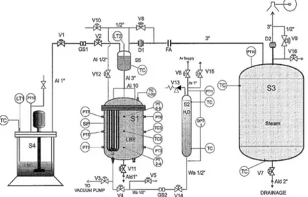
The original facility configuration is schematically shown in Fig.4.1. It has been adopted for performing Test n.1 of the IP-EUROTRANS campaign.

(2)

Fig.4.1 - Schematic representation of the original LIFUS 5 facility

It consisted of a reaction vessel (S1) where the interaction between LBE and water took place, an expansion vessel (S5) linked to the reaction vessel, a water tank (S2), a dump tank (S3) and a liquid metal storage tank (S4). Their main features are summarized in Table 4.1.

S1 - reaction tank

Volume 0.1 [m3]

Inner diameter 0.42 [m]

Design pressure 20 [MPa]

Design temperature 500 [◦C]

Material AISI 316

S2 - water tank

Volume 0.015 [m3]

Inner diameter 4 in.sch.160 [in]

Material AISI 316

S3 - safety tank

Volume 2.0 [m3]

Inner diameter 1.0 [m]

Design pressure 1.0 [MPa]

Material AISI 316

S5 - expansion tank

Volume 10.1 [l]

Inner diameter 6 in.sch.160 [in]

Material AISI 316

(3)

89 The volume of the S1 vessel was 100 l and, inside it, there were two AISI 316 plates welded on the top flange (see Fig.4.2), dividing the internal volume into four sectors. The sectors were connected to each other through a gap of 0.05 m from the bottom of the vessel and, laterally, through a gap of 0.005 m. In addition, the four sectors of the reaction vessel S1 were connected to the expansion vessel S5, having a volume of 10 l, through four tubes placed on the top flange. Each tube had a total length of 0.33 m, an outer diameter of 0.017 m and a thickness of 0.003 m.

A mock-up of U shaped tubes, which consisted of 10 tubes of 0.0165 m of external diameter and about 0.7 m in length, was located in one of the four sectors described above. This mock-up was introduced to simulate the effects of steam generator tubes on the phenomena involved in the interaction between LBE and water (e.g. enhanced mixing).

Fig.4.2 - The reaction vessel with the tube bundle

The water injection device was placed at the bottom of S1, in the sector containing the mock-up of U tubes. It consisted of a 1/2 in. tube, with an orifice of 0.004 m on the top, which extended for 0.08 m into the reaction vessel.

The orifice was covered by a protective cap which was broken by the pressure of the water jet at the beginning of the injection phase.

Depending on the LBE filling level, the compressibility of the whole volume (S1 plus S5) could be varied, giving the possibility of evaluating the different responses of the system in terms of pressure evolution.

The S2 tank contained pressurized water to be injected in S1 through the 1/2 in. pipeline. During the test the pressure in S2 was kept fixed by connecting directly this vessel to an Argon bottle charged at the test pressure.

The dump tank S3 volume was equal to 2 m3 and the design pressure was 1MPa. The S3 vessel represents a safety volume used to collect the gaseous and aerosol reaction products from S5 at the end of the test.

Furthermore, it protected the system during the injection phase by means of the rupture disk D1 set at 19 MPa.

(4)

The liquid metal storage tank S4 contained the melted LBE and transferred from S4 to S1 during the load operations of the facility.

The following instrumentation was adopted for test n.1:

• 18 K-type quick response thermocouples placed on the tube bundle of S1. The thermocouples were equally spaced within 0.2 m in the vertical direction, starting from 0.05m above the lowest point of the U tubes of the mock-up (see

Fig.4.3 )

• a low response time socket thermocouple placed in S5;

• 7 pressure transducers in S1; two pressure transducers were placed along the vessel wall of the sector containing the mock-up of U tubes and the other five pressure transducers were placed on the vessel wall of the other three sectors; • 1 pressure transducer placed on the wall of S5;

• 1 pressure transducer placed on the water pipe just before its entry in S1.

Fig.4.3 - Cross section of the reaction vessel with the indication of the tubes equipped with thermocouples are placed (above) and axial distribution of the thermocouples (below).

All the pressure sensors were water-cooled, high precision, piezometric transducers (type 7061B supplied by Kistler Company). Their relatively short time constant (about 10−4 s) allowed monitoring the rapid pressure transients in the system under a time scale of some seconds. A differential pressure sensor for the

(5)

91 water levels measurement was placed in S2, too. Unfortunately, for some test the data collected by this sensor were not available due to its partial failure.

A fast data acquisition system (DAQ) with dedicated software in LabVIEW environment acquired the main test parameters during all the phases of the experiment. All the operations of the facility control and the supervision were carried out by means of a PLC system integrated with a PC, which allows the settings of the control and alarm parameters, such as temperature, pressure, liquid metal and water level, through the synoptic display of the facility. A more detailed description of the facility is available in [1].

The main operating conditions of the Test n.1 are summarized in the following. They were chosen on the basis of the preliminary indications concerning the working parameters of XT-ADS steam generator [149].

Thermodynamic parameters

• Liquid metal temperature: 350°C;

• Initial pressure on the liquid metal free level: 0.1 MPa; • Water injection pressure: 7 MPa;

• Water temperature: 235°C (subcooling of about 50 ° C). Reaction system

• Free volume in the expansion vessel: 5 l; • Liquid metal volume: 105 l.

Injection system

• Duration of the test (V14 open): 10 s;

• Diameter of the injection device (water orifice): 0.004 m; • Water injector device penetration inside S1: 0.08 m.

The test was performed following three main operational phases.

The first one was the so called “pre-test phase”, during which the LBE quantity was loaded from S4 and maintained to the temperature fixed for the test and the S2 tank was filled with water and pressurized by the argon.

The second (and main) one was the “test phase” which started with the opening of V14 valve and continued with the water injection, finishing after 10 s with the V14 closure.

The last one was the “post-test phase” during which, after the collection of the gaseous products in S3, liquid metal was drained in S4 and cooled under inert atmosphere.

4.2.2 Changes to the facility and operating conditions for the other

experiments

4.2.2.1 Test n.2

As previously mentioned, the original configuration of the facility has been adopted for Test n.1 only.

For Test n.2, the facility was changed by eliminating the S5 tank, as shown in Fig.4.1. This modification was aimed at investigating possible consequences of LBE-water interaction in representative conditions for ICE (Integral Circulation Experiments), an experimental activity planned in CIRCE facility, which is also located in ENEA Brasimone [8,10]. In particular, this experiment was designed in

(6)

order to couple a heat source with a cold sink in a pool configuration similar to the geometry of reactors under development.

S2

Fig.4.4 - Layout of the modified LIFUS 5 facility

The main operating conditions of the Test n.2 are summarized in the following.

• Liquid metal temperature: 350 °C;

• Initial pressure on the liquid metal free level: 0.1 MPa; • Water injection pressure: 0.6 MPa;

• Water temperature: 130 °C (subcooling of about 28 °C). Reaction system

• No expansion vessel S5; • Liquid metal volume: 80 l;

• Free volume with respect LBE volume inside S1: 20 l (20 %). Injection system

• Diameter of the injection device (water orifice): 0.008 m (nominal); • Water injector device penetration inside S1: 0.06 m-

It must be pointed out that this test was partially unsuccessful, because of the failure of the opening of the injection.

A consecutive examination of the injector device explained the discrepancies between experimental and simulation results has highlighted the actual reduction of the orifice with respect to its nominal diameter [11].

4.2.2.2 Test n. 3, n. 4 and Test n.1 and n.2 for ELSY Program

The next tests carried out on the LIFUS 5 facility were performed with the same facility configuration (see Fig.4.1). Therefore, for the sake of simplicity, the description of these tests is considered altogether.

The main facility’s feature for all these tests was the direct connection of reaction vessel S1 with safety vessel through a discharge line. It was built using a

(7)

93 3” sch. 80 tube (outer diameter 88.9 mm, thickness 7.62 mm) made of AISI 316L, two welding neck flanges and three 90° elbows, as s hown in Fig.4.5.

Fig.4.5 - LIFUS 5 configuration adopted for Test n.3 and n.4 of IP-EUROTRANS Project and Test n.1 and n.2 of ELSY Experimental Program

This change was performed in order to study the consequences of a possible discharge of water vapour/liquid metal mixture outside the steam generator module because of a tube rupture accident that might occur in HLMR reactors [12]. In addition to this, the four welded plates inside S1 (see Fig.4.2) have been removed. The operating conditions for Test n.3 were the following.

• Liquid metal temperature: 350 °C;

• Water temperature: 235 °C. Reaction system

• No expansion vessel S5, direct discharge in S3 through a discharge line; • Liquid metal volume: 100 l;

• No free volume with respect LBE volume inside S1. Injection system

• Diameter of the injection device (water orifice): 0.004 m (nominal); • Water injector device penetration inside S1: 0.05 m.

Concerning Test n.4, the operating conditions were the same, except for the ratio between the free volume and LBE volume inside S1 fixed at 20 l, that is 20 % of S1 volume. With reference to Test n.1 and Test n.2 of the ELSY Experimental Program, the operating conditions are summarized below.

(8)

• Water temperature: 325 °C (subcooling of about 2 °C). Reaction system

• No expansion vessel S5, direct discharge in S3 through a discharge line; • Liquid metal volume: 80 l;

• Free volume with respect LBE volume inside S1: 20 l. Injection system

• Diameter of the injection device (water orifice): 0.004 m (nominal); • Water injector device penetration inside S1: 0.005 m.

It must be pointed out that the location of the injection device in this test has been taken as close as possible to the bottom of the S1 vessel. On the contrary, Test n. 2 has been carried out with the same operating conditions except for the penetration of the injection device, which has been placed at 0.5 m from the bottom of the vessel. This has allowed to analyse the influence of a hypothetic tube rupture occurring in an upper position of the steam generator.

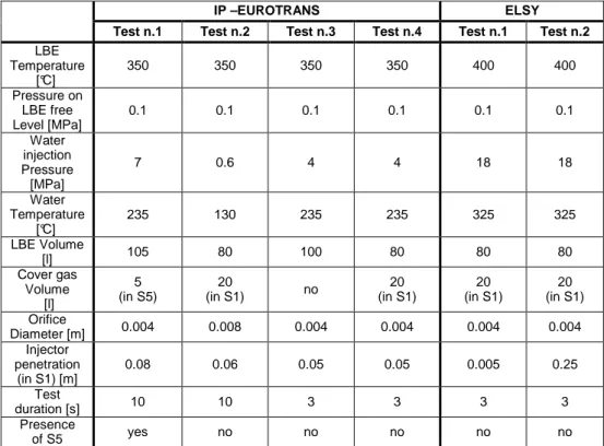
In Table 4.2 all the experimental conditions of the two campaigns are summarized.

IP –EUROTRANS ELSY

Test n.1 Test n.2 Test n.3 Test n.4 Test n.1 Test n.2

LBE Temperature [°C] 350 350 350 350 400 400 Pressure on LBE free Level [MPa] 0.1 0.1 0.1 0.1 0.1 0.1 Water injection Pressure [MPa] 7 0.6 4 4 18 18 Water Temperature [°C] 235 130 235 235 325 325 LBE Volume [l] 105 80 100 80 80 80 Cover gas Volume [l] 5 (in S5) 20 (in S1) no 20 (in S1) 20 (in S1) 20 (in S1) Orifice Diameter [m] 0.004 0.008 0.004 0.004 0.004 0.004 Injector penetration (in S1) [m] 0.08 0.06 0.05 0.05 0.005 0.25 Test duration [s] 10 10 3 3 3 3 Presence of S5 yes no no no no no

(9)

95

4.3 Numerical simulation and comparison with experimental

results

4.3.1 Geometrical model development and code qualification

4.3.1.1 Test n.1

In a simulation activity performed at University of Pisa the experimental results have been analysed using the SIMMER III code in order to get a deeper understanding of the operating conditions. .

Using SIMMER III, a two-dimensional code, the setup of the numerical model of LIFUS 5 facility presented some difficulties. In fact, the LIFUS 5 test section was characterized by geometrical features which originated evident asymmetries.

In particular, the elements which created the main problems were the subdivision of the S1 vessel into four parts by plates, the presence of the injection device and of U tubes in only one sector of S1 and the four tubes (one tube for each sector) that connected the S1 to the S5 tank.

Furthermore the presence of the gap between the tank wall and the plates, which allowed LBE to flow through the sectors, complicated even more the situation.

These complex characteristics of the facility compelled to simplify the geometry to be used for SIMMER III simulations making some assumptions. In particular, two different 2D geometrical models of LIFUS facility have been developed on the basis of Test n.1 findings.

The first one, called CM1 (see Fig.4.6), was obtained through a more simplified representation of the domain with respect to the second one, called CM2 (see

Fig.4.7) which was more detailed in order to try to improve the results of the

simulations [13].

(10)

Fig.4.7 - LIFUS 5 computational domain CM2

The experimental results concerning pressure and temperature have been compared with the simulations findings in order to qualify the code [13]. This comparison also helped in deciding which one the models was most suitable for simulating the next tests.

In Fig.4.8and Fig.4.9the comparison between the experimental and CM1 and CM2 pressure trends in S1 and S5 tank, respectively, is shown.

The starting time (t = 0) chosen for the comparison corresponds to the time in which the water injection in S1 starts.

0.E+00 1.E+06 2.E+06 3.E+06 4.E+06 5.E+06 6.E+06 7.E+06 8.E+06 9.E+06 0 2 4 6 8 10 12 Time [s] P re s s u re [ P a ] Experiment CM1 CM2

(11)

97 0.E+00 1.E+06 2.E+06 3.E+06 4.E+06 5.E+06 6.E+06 7.E+06 8.E+06 0 2 4 6 8 10 12 Time [s] P re s s u re [ P a ] Experiment CM1 CM2

Fig.4.9 - Comparison between experimental and calculated result in S5

0.0E+00 1.0E+06 2.0E+06 3.0E+06 4.0E+06 5.0E+06 6.0E+06 7.0E+06 8.0E+06 9.0E+06 0 2 4 6 8 10 12 Time [s] P re s s u re [ P a ] S1 Pressure (Experiment) S5 Pressure (Experiment) S1 Pressure (CM2) S5 Pressure (CM2)

(12)

The three hystories (see Fig.4.8) are in quite good agreement, even though the code tends to slightly overestimate the experimental pressure. In both simulations, the second pressure peak in S1 shows a time delay, which is partially due to the geometrical simplifications adopted in the domain, such as the representation of the mock-up of the U tubes and the presence of the S1–S5 central connection tube. This feature affects the delay observed and the slope of the depressurization phase of CM2 model, also.

Pressure trends in S5 tank (see Fig.4.9) highlighted a better agreement between CM2 simulation and the experimental results, as shown in Fig.4.10, reproducing “pressure coupling”. Temperature trends of the cells corresponding to the various positions of the thermocouples have been compared for both models, too [8, 14]. For the sake of simplicity, in the following, only the comparison concerning temperature trends of the injector’s closest thermocouples have been shown.

Similar to what observed for pressure trends, the experimental results are in a better agreement with CM2 model, as can be seen in Fig.4.11, Fig.4.12 and

Fig.4.13. Bottom Thermocouple 240 260 280 300 320 340 360 0 2 4 6 8 10 12

Time [s]

T

e

m

p

e

ra

tu

re

[

°C

]

Experiment CM1 CM2

(13)

99 Middle Thermocouple 240 260 280 300 320 340 360 0 2 4 6 8 10 12

Time [s]

T

e

m

p

e

ra

tu

re

[

°C

]

Experiment CM1 CM2

Fig.4.12 - Middle thermocouple

Top Thermocouple 240 260 280 300 320 340 360 0 2 4 6 8 10 12 Time [s] T e m p e ra tu re [ °C ] Experiment CM1 CM2

(14)

Therefore, in the light of this post test analysis, CM2 was chosen as the reference model for the pre- and post-test analysis of the next tests carried out on the LIFUS 5 facility.

4.3.1.2 Test n.2

As mentioned, Test n. 2 was carried out removing the S5 vessel. Therefore, the geometrical domain set up for Test n.1 required appropriate modifications in order to perform simulations. In Fig.4.14 and Fig.4.15 are shown the facility configuration’s scheme set up for Test n.2 and the corresponding modification of the geometrical model, respectively.

Fig.4.14 - LIFUS 5 configuration for Test n.2

(15)

101 Despite this test has been partially unsuccessful because of the partial failure of the opening of the injector device, the simulation activity helped to understand the problem occurred, revealing the discrepancies between experimental results and the nominal conditions [11].

In particular, the simulations exhibited differences in pressure histories, inducing to evaluate the likelihood of a smaller water injection with respect to what had been calculated with the nominal orifice diameter of 8 mm (see Fig.4.16). After several attempts, pressure histories derived from an orifice diameter of about 4 mm turned out as the closest to experimental results (see Fig.4.17).

0.0E+00 2.0E+05 4.0E+05 6.0E+05 8.0E+05 1.0E+06 1.2E+06 1.4E+06 1.6E+06 1.8E+06 2.0E+06 0.0 2.0 4.0 6.0 8.0 10.0

Time [s]

P

re

s

u

re

[

P

a

]

Experiment SIMMER III

Fig.4.16 - Comparison between experimental and simulation results under nominal conditions (orifice diameter 4 mm)

(16)

0.0E+00 2.0E+05 4.0E+05 6.0E+05 8.0E+05 1.0E+06 1.2E+06 1.4E+06 1.6E+06 1.8E+06 2.0E+06 0.0 2.0 4.0 6.0 8.0 10.0 Time [s] P re s s u re [ P a ] Experiment SIMMER III

Fig.4.17 - Comparison between experimental and simulation results under supposed actual condition (orifice diameter 4 mm)

This result was confirmed from the comparisons between experimental and simulated temperatures, which are shown in Fig.4.18, Fig.4.19 and Fig.4.20 for the injector’s closest thermocouples.

120 160 200 240 280 320 360 0.0 2.0 4.0 6.0 8.0 10.0 Time [s] T e m p e ra tu re [ °C ] TC18 (Bottom- tube n.3) SIMMER III

(17)

103 120 160 200 240 280 320 360 0.0 2.0 4.0 6.0 8.0 10.0

Time [s]

T

e

m

p

e

ra

tu

re

[

°C

]

TC17 Middle- tube n.3 SIMMER III

Fig.4.19 - Middle thermocouple

120 160 200 240 280 320 360 0.0 2.0 4.0 6.0 8.0 10.0

Time [s]

T

e

m

p

e

ra

tu

re

[

°C

]

TC16 (Top- tube n.3) SIMMER III

(18)

Thus, it must be pointed out that the information from this test must be considered only partially in the study concerning LBE-water interaction.

4.3.1.3 Test n. 3 and n. 4

The last two tests of the IP-EUROTRANS Program have been grouped together because they have been carried out with the same facility configuration. The only difference was the amount of LBE inside S1 that in case of Test n. 3 filled the vessel completely, while in Test n. 4 filled 80% of the total S1 volume. The two calculational domains developed for these simulations are shown in Fig.4.21 and in

Fig.4.22.

(19)

105

Fig.4.22 - LIFUS 5 configuration for Test n.4

The same domain of the previous simulation (Test n.2) was used for S1 and S2 vessel and the injection line.

The line which connected directly S1 to S3 and S3 vessel has been added in the domain, keeping volumes and, for the connection pipe, also the flow area. The comparison between experimental and simulated pressure data for Test n.3 and Test n. 4 are shown in Fig.4.23 and Fig.4.24 , respectively.

(20)

0.0E+00 5.0E+05 1.0E+06 1.5E+06 2.0E+06 2.5E+06 0 0.2 0.4 0.6 0.8 1 1.2 1.4 1.6 1.8 2 2.2 2.4 2.6 2.8 3 Time [s] P re s s u re [ P a ] Experiment SIMMER

Fig.4.23 - Comparison between experimental and simulation results for Test n.3

0.0E+00 2.0E+05 4.0E+05 6.0E+05 8.0E+05 1.0E+06 1.2E+06 1.4E+06 1.6E+06 1.8E+06 2.0E+06 0 0.2 0.4 0.6 0.8 1 1.2 1.4 1.6 1.8 2 2.2 2.4 2.6 2.8 3 Time [s] P re s s u re [ P a ] Experiment SIMMER

(21)

107 As can be seen, Test n.3 simulation reaches the maximum peak earlier than in experiment. In addition, this peak is slightly overestimated. An overestimation of the maximum pressure can be noted also in Test n.4, even though in this case the timing of the pressurization and depressurization phase is similar to the experimental one. In both cases, the depressurization phase approaches experimental pressure values. The discrepancies observed are mainly due to the simplifications adopted in setting up the domain.

The comparison of Test n. 3 temperature histories (see Fig.4.25, Fig.4.26 and Fig.4.27) has shown a good agreement between experimental and simulation data, despite simulation reveals a more oscillating trend.

TC18 0 50 100 150 200 250 300 350 400 0 0.5 1 1.5 2 2.5 3 Time [s] T e m p e ra tu re [ ◦ C ] Experiment SIMMER

(22)

TC17 0 50 100 150 200 250 300 350 400 0 0.5 1 1.5 2 2.5 3 Time [s] T e m p e ra tu re [ ◦ C ] Experiment SIMMER

Fig.4.26 - Middle thermocouple (Test n.3)

(23)

109 In similarity with Test n.3, Test n.4 showed a good agreement between experimental and calculated results, as can be seen in Fig.4.28, Fig.4.29 and

Fig.4.30.

.Also in this case, a more oscillating trend has been observed in the results of the simulation, in particular in the cell corresponding to the bottom thermocouple. These oscillations might be due to the larger amount of vaporization estimated by the code, which affects also the pressure results.

Fig.4.28 - Bottom thermocouple (Test n.4)

(24)

Fig.4.30 - Top thermocouple (Test n.4)

4.3.1.4 Test n.1 and n.2 for ELSY Campaign

The geometrical model used for simulating the first test carried out for ELSY campaign was the same used in Test n.4 of IP-EUROTRANS campaign (see

Fig.4.22) because the configuration of the facility for these two tests was the same.

The model developed for the Test n.2 was changed just in the length of the injector device. Thus, a magnification of S1 vessel model is given in Fig.4.31 and Fig.4.32.

(25)

111

Fig.4.32 - S1 configuration for Test n.2

Pressure data comparisons of the two tests are shown in Fig.4.33 and Fig.4.34

0.0E+00 5.0E+05 1.0E+06 1.5E+06 2.0E+06 2.5E+06 3.0E+06 3.5E+06 0 0.5 1 1.5 2 2.5 3 Time [s] P re s s u re [ P a ] Experiment SIMMER III

Fig.4.33 - Comparison between experimental and simulation results for ELSY Test n.1

(26)

0.0E+00 5.0E+05 1.0E+06 1.5E+06 2.0E+06 2.5E+06 3.0E+06 0.0 0.5 1.0 1.5 2.0 2.5 3.0 Time [ms] P re s s u re [ P a ] Experimental SIMMER III

Fig.4.34 - Comparison between experimental and simulation results for ELSY Test n.2

As can be seen, experimental and simulation curves are in good agreement. In particular Test n.1 has highlighted similar values for pressure peak and same timing, even though a slight overestimation of the first part of the depressurization phase (from 0.75 s to 1.5 s) can be noted. Test n.2 highlighted a slight overestimation of the pressure peak and of the first part of the depressurization phase (up to 1.5 s), while a general good agreement in timing can be observed.

An agreement on temperature decrease can be observed in temperature comparison of Test n.1 (see Fig.4.35, Fig.4.36 and Fig.4.37), although the simulation shows a more oscillating trend, similar to what observed in the last two tests of IP-EUROTRANS campaign.

(27)

113 TC18 0 50 100 150 200 250 300 350 400 450 0 0.5 1 1.5 2 2.5 3 Time [s] T e m p e ra tu re [ °C ] Experiment SIMMER

Fig.4.35 - Bottom thermocouple (Test n.1)

TC17 0 50 100 150 200 250 300 350 400 450 0 0.5 1 1.5 2 2.5 3 Time [s] T e m p e ra tu re [ °C ] Experiment SIMMER

(28)

TC16 0 50 100 150 200 250 300 350 400 450 0 0.5 1 1.5 2 2.5 3 Time [s] Te m pe ra tur e [ °C ] Experiment SIMMER

In Test n.2 just two thermocouples (respectively middle and top thermocouples TC17 and TC18, see also Fig.4.3) are placed on the tube closest to the injector device. Also in this case, simulation results have shown an oscillatory trend even more marked than in the previous simulation, especially for pronounced thermocouple n.17 being the closest to the injector device.

TC17 0 50 100 150 200 250 300 350 400 450 0 0.5 1 1.5 2 2.5 3 Time [s] T e m p e ra tu re [ °C ] Experiment SIMMER III

(29)

115 TC16 0 50 100 150 200 250 300 350 400 450 0 0.5 1 1.5 2 2.5 3 Time [s] T e m p e ra tu re [ °C ] Experiment SIMMER III

4.3.2 Concluding remarks of the model qualification activity

Since the LIFUS 5 facility configurations show evident asymmetries originating from their complex geometrical features some simplifications were needed for SIMMER 2-D geometrical simulations approach.

The simultation models, taking into account all the difficulties encountered, have generally highlighted a good agreement with experimental results, turning out as a helpful feedback for improving the experimental set up. Therefore, they have also been the basis for a better understanding of the interaction phenomena, which will presented in the following.

4.4 Analysis of the phenomena involved in LBE-water

interaction

All the experimental transients except Test n.1, as can be seen in Fig.4.40, have highlighted pressure trends in LBE characterized by two main phases: a first pressure peak with a rapid depressurization and a second pressurization with the consecutive depressurization, which is slower than the previous depressurization.

The first sharp peak, which can be noted in every test, is due to the impact of water on the LBE. Most of the amount of the water jet (estimated from simulations around 60-70%, in general) vaporises after fragmentation due to the sudden heat exchange between the two fluids.

The vapour produced during this first interaction pushes the LBE mass upwards, but when the flow rate is not anymore sufficient to balance the LBE pressure a rapid depressurization begins. Once the two fluid’s pressure is balanced, a further

(30)

water injection with consequent vapour production starts and a new pressurization take place. The pressure maximum is reached followed by a slow depressurization phase.

Concerning Test n.1, the pressure trend in S1 has highlighted several differences due to the completely different configuration of the facility (compare

Fig.4.1 and Fig.4.4) with respect to the other tests performed. The analysis of Test

n.1 transients is explained in detail in [13].

In the light of this, findings from simulations of Test n.1 and Test n.2, in which problems were observed as mentioned previously, will be partially considered for the tests analysis. Therefore, the tests considered will be Test n.3 and n.4 of the IP-EUROTRANS campaign and Test n.1 and n.2 for ELSY campaign. 0.0E+00 1.0E+06 2.0E+06 3.0E+06 4.0E+06 5.0E+06 6.0E+06 7.0E+06 8.0E+06 0 0.25 0.5 0.75 1 1.25 1.5 1.75 2 Time [s] P re s s u re [ P a ] Test n.1 Test n.2 Test n.3 Test n.4

Test n.1 ELSY Test n.2 ELSY

First peak and depressurization

Fig.4.40 - Pressure histories in S1 vessel during the first two seconds of experiments

It must be pointed out that the first peak (see again Fig.4.40), represents one of the most important concerns for safety issues. In fact this peak is due to the shock wave deriving from the sudden water injection that in HLMRs might occur because of a SGTR.

In relation to this phase, questions arise on the energy potential of this pressure waves and the likelihood of damaging surrounding structures like adjacent tubes of the SG causing a damage propagation that could potentially heavily damage the overall reactor.

In addition, the rapid vaporization following the rupture could cause the sloshing of the HLM pool and the steam transport through the core, thus introducing reactivity due to the core voiding.

(31)

117 Therefore, the analysis, the characterization and the energy evaluation of this peak plays a crucial role in HLMRs design.

As can be seen in Fig.4.41, all the tests performed in the two campaigns highlighted the presence of the shock wave’s peak in a time range of 0.01 s. In particular, Test n. 1, n.3, n. 4 and ELSY n. 1 show a same timing and almost the same shape of the pressure curve in reaching the maximum, while Test n. 2 reveals a slight delay, which becomes larger for ELSY Test n.2. In the latter two cases, the maximum peak’s values are considerable lower than in the other cases.

0.0E+00 5.0E+05 1.0E+06 1.5E+06 2.0E+06 2.5E+06 0 0.002 0.004 0.006 0.008 0.01 Time [s] P re s s u re [ P a ] Test n.1 Test n.2 Test n.3 Test n.4 Test n.1 ELSY Test n.2 ELSY

Fig.4.41- Pressure wave peak magnification (from experimental data)

It is important to note that the maximum shock wave peak corresponds to a flow rate peak, which in most of cases reaches the the maximum flow rate injected in the LBE pool (Test n.1, n.2, n.4, ELSY Test n.1, see Fig.4.42 and Fig.4.43). Unfortunately no experimental flow rate measurements are available, therefore this conjecture and the following analysis have been carried out on the basis of the SIMMER III simulations previously presented.

In particular, for Test n.1, in order to assess the correctness of flow rates estimated by SIMMER, a comparison between SIMMER and RELAP 5.3 simulations have been performed [15], revealing a good agreement between the findings of the two codes. Considering the six tests, it is possible to note, as expected, that water jet velocity trends have a shape similar to water flow rate trends because of their proportionality (compare Fig.4.43 with Fig.4.44).

(32)

0.0E+00 2.0E-01 4.0E-01 6.0E-01 8.0E-01 1.0E+00 1.2E+00 1.4E+00 1.6E+00 0.0 0.1 0.2 0.3 0.4 0.5 Time [s] F lo w r a te [ k g /s ] Test n.1 Test n.2 Test n.3 Test n.4

ELSY Test n.1 ELSY Test n.2

Fig.4.42 - Estimated flow rate during 0.5 s (from simulations)

0.0E+00 2.0E-01 4.0E-01 6.0E-01 8.0E-01 1.0E+00 1.2E+00 1.4E+00 1.6E+00 0.00 0.01 0.02 0.03 0.04 0.05 Time [s] F lo w r a te [ k g /s ] Test n.1 Test n.2 Test n.3 Test n.4 ELSY Test n.1 ELSY Test n.2

(33)

119 0.0E+00 2.0E+01 4.0E+01 6.0E+01 8.0E+01 1.0E+02 1.2E+02 1.4E+02 1.6E+02 1.8E+02 0.00 0.01 0.02 0.03 0.04 0.05 Time [s] J e t V e lo c it y [ m /s ] Test n.1 Test n.2 Test n.3 Test n.4 ELSY Test n.1 ELSY Test n.2

Fig.4.44 - Water jet velocity during 0.05 s

Focusing on Test n. 3 and Test n.4, which have been carried out under the same initial conditions (TLBE = 350 °C, Twater = 235 °C, Pinjection = 4 MPa, see also Table 4.2) except for the amount of argon in S1 vessel (20 l for Test n.4, no cover

gas for Test n.3), it is possible to note that the presence of the cover gas affects water jet velocity and the amount of water that vaporises.

As can be seen in Fig.4.45, water jet velocity shows a steep slope during the first 0.005 s in both cases, even though it is steeper for the test performed in absence of cover gas. After 0.005 s, in coincidence with pressure decrease, jet velocity shows a sudden slope decrease that for Test n.3 becomes a plateau. The water jet velocity starts to increase when the water pressure, after the balancing of the two fluids pressure, is again higher than LBE pressure, thus allowing new water injection. In any case, the maximum velocity value reached in test n.4 is higher than in Test n.3.

It is interesting to observe the calculated water volume fraction history in near the injection for both tests. In this case, Test n.3 highlighted a trend closer to that of jet velocity than in Test n.4, where after reaching a maximum, liquid water fraction begins to decrease thus showing a shape completely different from velocity trend. Considering the values (see Fig.4.46), it is possible to note that the amount of liquid water is higher in Test n.3 than in Test n.4, especially during the first milliseconds of injection (about 36% for Test n.3 and 24% for Test n.4 at 0.003 ms, see Fig.4.47 ).

(34)

0.0E+00 1.0E+01 2.0E+01 3.0E+01 4.0E+01 5.0E+01 6.0E+01 7.0E+01 8.0E+01 0.00 0.01 0.02 0.03 0.04 0.05 0.06 0.07 0.08 0.09 0.10 Time [s] J e t V e lo c it y [ m /s ] Test n.3 Test n.4 Cover gas in S1: 20 l No Cover gas in S1

Fig.4.45 - Water jet velocity over 0.05 s (Test n.3 e n.4)

0.00 0.05 0.10 0.15 0.20 0.25 0.30 0.35 0.40 0.00 0.01 0.02 0.03 0.04 0.05 Time [s] L iq u id v o lu m e f ra c ti o n Test n.3 Test n.4 No Cover gas in S1 Cover gas in S1 20 l

(35)

121 This is also confirmed by the estimation of the gas bubble growth, which has been evaluated through a dedicated tool written in FORTRAN, having a direct read access to the SIMMER III base file SIMBF, which has been validated in the experimental campaign SGI that will be presented in the next chapter. As can be seen in Fig.4.48 and Fig.4.49, the gas bubble, which is formed in S1 because of the sudden vaporization of injected water, increases more rapidly in Test n.4 rather than in Test n.3. 0.00 0.05 0.10 0.15 0.20 0.25 0.30 0.35 0.40 0.0000 0.0005 0.0010 0.0015 0.0020 0.0025 0.0030 Time [s] L iq u id v o lu m e f ra c ti o n Test n.3 Test n.4 Cover gas in S1 20 l No Cover gas in S1

Fig.4.47 - Water volume fraction during 0.003 s (Test n.3 e n.4)

0.0E+00 1.0E-05 2.0E-05 3.0E-05 4.0E-05 5.0E-05

0.0E+00 5.0E-04 1.0E-03 1.5E-03 2.0E-03 2.5E-03 3.0E-03

Time [s] B u b b le v o lu m e [ m 3] Test n.4 Test n.3 No Cover gas in S1 Cover gas in S1 20 l

(36)

0.0E+00 2.0E-03 4.0E-03 6.0E-03 8.0E-03 1.0E-02 1.2E-02 0.00 0.01 0.02 0.03 0.04 0.05 Time [s] B u b b le v o lu m e [ m 3] Test n.4 Test n.3 No Cover gas in S1 Cover gas in S1 20 l

Fig.4.49 - Bubble volume growth during 0.05 s (Test n.3 e n.4)

This might be explained as follows. The absence of cover gas opposes the movement of LBE that in Test n.3 condition can move upwards just through a small pipe. In this test, the lead cannot be easily displaced upwards offering water only little room to expand during vaporization.

Therefore, the heated water is mostly kept in a pressurized liquid state.

The transient up to 1 s (see from Fig.4.50 to Fig.4.51) shows that maximum pressure in Test n.3 is higher than in Test n.4, contrarily to what observed for the first peak where it overcomes the maximum pressure achieved during the second pressurization.

As mentioned before, the higher pressure is related to the stiffness of the system. The flow rate estimated by the code shows a decreasing trend that, after reaching the minimum in correspondence of maximum pressure, starts again to increase. It is clear that flow rate history is strictly linked to the pressure.

(37)

123 0.0E+00 4.0E+05 8.0E+05 1.2E+06 1.6E+06 2.0E+06 0 0.1 0.2 0.3 0.4 0.5 0.6 0.7 0.8 0.9 1 Time [s] P re s s u re [ P a ] Test n.3 Test n.4

Fig.4.50 - Pressure trend during 1 s (Test n.3 e n.4)

0.0E+00 1.0E-01 2.0E-01 3.0E-01 4.0E-01 5.0E-01 6.0E-01 7.0E-01 8.0E-01 0.0 0.1 0.2 0.3 0.4 0.5 0.6 0.7 0.8 0.9 1.0 Time [s] F lo w r a te [ k g /s ] Test n.3 Test n.4

Fig.4.51 - Flow rate during 1 s (Test n.3 e n.4)

As can be seen in Fig.4.52 and Fig.4.53 jet velocity and the amount of liquid water have complementary trends. In fact, when the velocity reaches its maximum the water volume fraction over the injector device reaches the minimum and vice versa.

(38)

Because of the higher amount of water injected within the first 100 ms, the total estimated injected water mass is higher in Test n.3 (1.64 kg) than in Test n.4 (1.43 kg).

The higher pressure peak is due to the stiffer system and limited potential to accommodate water in vapour state.

0.0E+00 1.0E+01 2.0E+01 3.0E+01 4.0E+01 5.0E+01 6.0E+01 7.0E+01

0.00E+00 1.65E-01 5.22E-01 7.30E-01 8.02E-01 8.40E-01 8.63E-01 8.84E-01 9.07E-01 9.41E-01

Time [s] J e t v e lo c it y [ m /s ] 0.0E+00 1.0E-01 2.0E-01 3.0E-01 4.0E-01 5.0E-01 6.0E-01 7.0E-01 8.0E-01 9.0E-01 1.0E+00 L iq u id v o lu m e f ra c ti o n Jet velocity

Liquid volume fraction No Cover gas in S1

Fig.4.52 - Jet velocity (thick line) and water volume fraction over 1 s

0.0E+00 1.0E+01 2.0E+01 3.0E+01 4.0E+01 5.0E+01 6.0E+01 7.0E+01 8.0E+01

0.00E+00 1.65E-01 5.22E-01 7.30E-01 8.02E-01 8.40E-01 8.63E-01 8.84E-01 9.07E-01 9.41E-01 Time [s] J e t v e lo c it y [ m /s ] 0.0E+00 1.0E-01 2.0E-01 3.0E-01 4.0E-01 5.0E-01 6.0E-01 7.0E-01 8.0E-01 9.0E-01 1.0E+00 L iq u id v o lu m e f ra c ti o n Jet velocity

Liquid volume fraction Cover gas in S1: 20

(39)

125 Therefore from these two tests, it is possible to deduce that the presence of cover gas might play a role in mitigating the effects of a shock wave peak. The impact of different position of the tube rupture plane has been investigated in the ELSY campaign where two test have been carried out with the same initial conditions (TLBE = 400 °C, Twater = 350 °C, Pinjection = 18 MPa, 20 l of argon inside

S1, see Table 4.2 also) but with a different injector device length.

As can be observed in Fig.4.54, the trends of the water jet velocity are similar, showing a similar timing also, even though velocity values are lower in case of long injector device. Focusing on the first 0.01 s, which is the time range where the peak of the shock wave takes place, it is possible to see that the volume of vapour produced in the interaction, shown in Fig.4.55, is higher if the injector device is shorter. 0.0E+00 2.0E+01 4.0E+01 6.0E+01 8.0E+01 1.0E+02 1.2E+02 1.4E+02 1.6E+02 1.8E+02 0.00 0.01 0.02 0.03 0.04 0.05 0.06 0.07 0.08 0.09 0.10 Time [s] J e t V e lo c it y [ m /s ] ELSY Test n.1 ELSY Test n.2 Long Injector Short Injector

Fig.4.54 - Water jet velocity during 0.05 s (ELSY Campaign)

0.0E+00 2.0E-04 4.0E-04 6.0E-04 8.0E-04 1.0E-03 1.2E-03 0.000 0.001 0.002 0.003 0.004 0.005 0.006 0.007 0.008 0.009 0.010 Time [s] B u b b le v o lu m e [ m 3] ELSY Test n.1 ELSY Test n.2 Long Injector Short Injector

(40)

This can be easily explained because the water injected through a short injector is in touch with the LBE for a longer time. Therefore water has more possibility to take heat from LBE and vaporise. On a longer time, flow rate tends to decrease (see again Fig.4.42) as well as the jet velocity trend (see Fig.4.56).

It is worth noting that the liquid volume fraction in the zone above the injection device has a higher value in case of long injection (see Fig.4.57). This tendency is confirmed from the evaluation of the overall water mass injected that is estimated as 2.4 kg for Test n.1 and 1.4 kg for Test n.2. In particular, during the first 0.25 s Test n.2 values are higher than in Test n.1 and then they tend to be equal. A possible explanation of this fact is that in case of longer injections, the LBE mass available for interacting with water is smaller than in the other case, allowing less vaporisation and letting a bigger amount of water in the liquid state.

It is interesting to make further comments comparing the tests carried out in the two experimental campaigns, although the change of several parameters (i.e. pressure injection, water and LBE temperature, etc.) at the same time and the limited number of tests makes it a little bit difficult. First of all it is possible to compare the tests of the two campaigns where a cover gas volume of 20 l in S1 is present (respectively, Test n.2, Test n.4, ELSY Test n.1 and ELSY Test n.2). Test n.2 of IP-EUROTRANS campaign is taken into account assuming that the orifice diameter is 4 mm.

Comparing all these tests it is possible to note that changing the injection pressure, both maximum flow rate and overall injected water mass are affected by the injector length that in both cases limits these two quantities, as can be observed from Fig.4.58 and Fig.4.59.

20% Argon in S1 0.0 0.2 0.4 0.6 0.8 1.0 1.2 1.4 1.6 0 2 4 6 8 10 12 14 16 18 20

Injection Presssure [MPa]

M a x im u m F lo w r a te [ k g /s ] Short injector device Long injector device

Fig.4.56 - Pressure-Maximum flow rate in presence of 20 l Argon in S1

(41)

127 20% Argon in S1 0.0 0.5 1.0 1.5 2.0 2.5 3.0 0 2 4 6 8 10 12 14 16 18 20

Injection Presssure [MPa]

W a te r M a s s I n je c te d [ k g /s ] Short injector device Long injector device

Fig.4.57 - Pressure-Injected Water mass in presence of 20 l Argon in S1

Further comments can be done focusing on the subcooling of the injected water. In Fig.4.60, the difference between maximum pressures reached in the tests and the injection pressure and the difference between the shock wave peak pressure and injection pressure have been considered as a function of water subcooling for Test n.3, n.4 and both the ELSY Tests.

-18.0 -15.0 -12.0 -9.0 -6.0 -3.0 0.0 0 2 4 6 8 10 12 14 16 Water Subcooling [°C ] P re s s u re d if fe re n c e [ M P a ]

Maximum Pressure-Injection Pressure Peak Pressure-Injection pressure Trendline Trendline ELSY Test n.1 & n.2 Test n.3 & n.4

Fig.4.58 - Subcooling Degree - Pressure difference for Test n.3 & n.4 and ELSY Test n.1 & n.2

(42)

-18.0 -15.0 -12.0 -9.0 -6.0 -3.0 0.0 3.0 6.0 0 13 26 39 52 Water Subcooling [°C ] P re s s u re d if fe re n c e [ M P a ]

Maximum Pressure-Injection Pressure Peak Pressure-Injection pressure Trendline

Trendline

Fig.4.59 - Subcooling Degree - Pressure difference (all tests)

As can be seen the two trends tends to converge. In fact, increasing water subcooling the pressure difference based on the maxima increases as well as the pressure difference based on shock wave peak. Adding to the figure the data of Test n.1 and Test n.2, as in Fig.4.61, it is possible to see that the convergence point is in proximity of Test n.2 and after reaching that point the two curves tends to diverge again.

Thus, it seems to be possible the existence of a water subcooling value (or at least of a small range of water subcooling values) for which both the shock wave peak pressure and the maximum pressure caused by the interaction do not exceed initial pressure conditions of the water injected. In order to clarify things, let us suppose, for instance, to inject a certain amount of water having a subcooling of 26 degrees in a heavy liquid metal pool. Referring to Fig.4.59, for this subcooling degree, the difference between the maximum pressure and the pressure of the water injected is about zero, as well as for the pressure peak due to the shock wave. Thus it is possible to know the maximum pressures reached from the initial condition of the water injected.

Comparing the subcooling degree-injection pressure curve (Fig.4.62) obtained from the initial water injection conditions (reference curve) with the same curve obtained from the maximum pressures reached in the experiments, it is possible to note the influence of the injector’s length and of the presence of cover gas in S1. On the light of the results previously discussed, a short injector tends to move the curve nearer the reference curve because it allows reaching higher pressure as well as the absence of cover gas region. Therefore these two features may play a role in changing the curve’s slope.

(43)

129 From the comparison of Fig.4.64 and Fig.4.63 it is possible to note, as expected, that the subcooling degree-maximum estimated injection velocity curve shows a similar trend with respect to subcooling degree-injection pressure curve, which is in both cases expressed by a cubic relationship.

Maximum Pressure-Injection Pressure Peak Pressure-Injection pressure

Trendline Trendline ELSY Test n.1 & n.2 Test n.3 & n.4

Fig.4.60 - Subcooling Degree - injection pressure curves

Maximum Pressure-Injection Pressure Peak Pressure-Injection pressure Trendline Trendline ELSY Test n.1 & n.2 Test n.3 & n.4

Fig.4.61 - Subcooling Degree - Pressure difference for Test n.3 & n.4 and ELSY Test n.1 & n.2

(44)

0 2 4 6 8 10 12 14 16 18 20 0 10 20 30 40 50 60 Water Subcooling [°C] Pr e s s u re [ M Pa ] Injection Pressure Max pressure Trendline initial conditions

Trendline Maximum Short injector Long injector _{Ar 20 l} No Ar

Fig.4.62 - Subcooling degree -injection pressure curves

0 20 40 60 80 100 120 140 160 180 0 10 20 30 40 50 60 Water Subcooling [°C] J e t v e lo c it y [ m /s ]

(45)

131 Considering the two ELSY tests and Test n.4 (see Fig.4.64) and adding the Test n.2 results also (Fig.4.65), which means that all the tests performed with 20 l of Argon in S1 have been taken into account, it is possible to see that the shorter is the injector the higher is the maximum jet velocity.

Argon 20 l (20% overall volume)

0 20 40 60 80 100 120 140 160 180 0 2 4 6 8 10 12 14 16 Water Subcooling [°C] M a x im u m J e t V e lo c it y [ m /s ] Test n.4 ELSY Test n.2 ELSY Test n.1

Fig.4.64 - Subcooling degree - maximum injection velocity in presence of 20 l Argon injection pressure curves

Argon 20 l (20% overall volume)

0 20 40 60 80 100 120 140 160 180 0 5 10 15 20 25 30 Water Subcooling [°C] M a x im u m J e t V e lo c it y [ m /s ] Test n.2 Test n.4 ELSY Test n.2 ELSY Test n.1

Fig.4.65 - Subcooling degree - maximum injection velocity in presence of 20 l Argon injection pressure curves

(46)

4.4.1 Concluding remarks of analysis of the LBE-water interaction

Since the LIFUS 5 facility configuration used for carrying out the six tests under several different conditions was changed several times and more than one parameter was changed at the same time, observations and comments turn out to be quite difficult. In any case, also thanks to the simulation activity carried out, some conclusions have been possible.

First of all, the pressure peak deriving from the shock wave is one of the characteristic features of LBE-water interaction. In fact, its presence has been detected in all the tests performed. In coincidence with this peak in almost all tests, a maximum of water injected flow rate and of water jet velocity has been detected.

Comparing tests carried out under the same initial conditions but changing just one parameter, the influence of the presence of gas in the reaction vessel S1 (Test n.3 and n.4 of IP-EUROTRANS campaign) and of the injector length (ELSY Test n.1 and n.2), which has been aimed at representing diverse tube failure planes, have been analysed. It was that first peak may be slightly mitigated by the absence of cover gas region or by a longer injector device, representative of a less deep SG tube rupture’s point. In both cases, over the duration of the shock wave pressure, the amount of water that vaporizes is lower than in the other tests (compare Test n.3 to n.4 and ELSY Test n.1 to n.2). On a longer time, such as on the rest of the transient where the pressure maximum is achieved, a longer injector allows reducing pressures, confirming the same tendency seen for shock wave peak, while the absence of gas allow at increasing system’s pressure because of the limited possibility for the vapour produced to expand.

Another important result that emerged from the data is the existence of one value of water subcooling for which both shock wave peak pressure and maximum pressure caused by interaction does not exceed initial conditions. In addition, since pressure and water jet velocity are proportional, effects on pressures may be found also on the velocity.

4.5 Energy evaluation

4.5.1 The isentropic model

A first attempt to evaluate the energy release has been made through a thermodynamic approach, such as the isentropic model, explained in Chapter 3.

It is recalled that the isentropic model gives a conservative estimation of the work potential for postulated meltdown accidents. This work potential is set equal to the change in fuel internal energy during an isentropic expansion from a compressed state to an expanded state, without taking into account any kinetic process that may be involved.

In equation form it corresponds to

0 du

pdv

ds

T

+

=

(4.1) , . f mech isentr i f i

W

= −

∫

pdv

=

U

−

U

(4.2)

The basic concept of isentropic work potential is explained by a two component system of LBE and water (like we find in the LIFUS tests).

(47)

133 Between two control volumes, one containing hot LBE and one containing water, heat is exchanged until a thermal equilibrium is reached at a common temperature

T

e. Assuming a constant volume thermal equilibrium process, the control volumes

do not provide work to the environment.

For each component a specific T-s diagram is defined outlining the process from initial state 1 to thermal equilibrium state e. Fig.4.66 represents the control volume and heating process for water.

s

Water control element Heating process of water

Fig.4.66 - Control element and constant-volume heating for water

Similarly to what described above, LBE undergoes a constant volume cooling process from initial state 1 to the equilibrium temperature Te, sketched in

Fig.4.67.

s

LBE control element Cooling process of LBE

Fig.4.67 - Control element and constant-volume cooling for LBE

From the equilibrium state e, characterized by a common temperature Te, independent isentropic expansions to the final state 2 are assumed for LBE and water.

e

W1- e =0

(48)

The final state 2 is defined by either a common pressure or an available volume to which the two materials expand.

A final pressure of 1 bar, as shown in Fig.4.68, is considered as an expansion to the environment giving a theoretical upper limit for the mechanical work.

Fig.4.68 - Water-LBE interaction decomposed into steps: adiabatic heating/cooling and isentropic expansion

According to this model, the mechanical work corresponds to the summed contribution of isentropic expansions of LBE and of water, or the sum of changes of internal energies from initial to the final states, respectively 1 and 2.

(

)

(

)

, 1 2 1 2

mech isentr _LBE _water

W

=

U

−

U

+

U

−

U

(4.3)

The evaluation of Q (see again Fig.4.66 and Fig.4.67) can be performed applying the first law of thermodynamics for each control element.

Considering an isochoric change of state from 1 to e and neglecting potential and kinetic energy changes (thermodynamic approach) the first law gives for water and LBE, respectively e w

Q

U

=

_→

∆

1 (4.4) e LBE

Q

U

=

−

_→

∆

1 (4.5)

The internal energies expressed as functions of temperatures are

(

1

)

w w w w v e

U

m c

T

∆

=

−

(4.6)

(

1

)

LBE LBE LBE LBE v e

U

m

c

T

∆

=

−

(4.7)

Assuming that the interaction of the system LBE-water is adiabatic, from the combination of (4.6) and (4.7) follows

S

Water

S

(49)

135

(

1

)

(

1

)

w w LBE LBE

w v e LBE v e

m c

T

−

T

=

m

c

T

−

T

(4.8)

and from (4.8) we get the common equilibrium temperature

T

e from a mass

weighted averaging of the initial internal energies.

1 1 w w LBE LBE w LBE w v LBE v e w v LBE v

m c T

m

c

T

m c

m

c

+

=

+

(4.9)

In order to evaluate

W

mech,isentr, the quality x2 must be determined and the following

approach may be used.

The existing relation for the thermodynamic properties between two infinitesimally close equilibrium states is

vdp

dh

Tds

=

−

(4.10) which can be written for an isentropic approach as:

s s

T

dp

v

T

dh













=













(4.11) Making the assumption of the independence from the temperature, over the range of interest, of

c

p and

h

fg the enthalpy change for this isentropic expansion can be

expressed by

dx

h

dT

c

dh

=

_p

+

_fg (4.12) Neglecting the liquid specific volume and applying the perfect gas law result:

p

RT

x

xv

v

≡

_f

+

_fg

≈

_g

≈

(4.13) In an isentropic process, the differential of

p(T, s)

is

dT

T

p

dp

s













∂

=

(4.14) s

T

p













∂

may be expressed by using the Clausius- Clapeyron relation, which links parameters along the saturation line to the enthalpy and volume of vaporization, under the assumption that the state e is almost at the saturation line. Therefore the expansion is almost totally under the saturation dome and then