Chapter 3 Prediction of NO emissions in a pilot-scale burner

(1)

Chapter 3 Prediction of NO emissions in a

pilot-scale burner

This present Chapter describes the experimental and numerical activity carried out on an NG-fired pilot-scale burner, designed to operate in flame and flameless regime 1_{. However, the eﬀect of injection of ammonia (NH}

3) in flame through a

special probe has been also explored.

The Chapter starts with the description of the burner, followed by a brief sum-mary of the experimental campaigns carried out at Enel Ricerca in Livorno, Italy. Then, the numerical modeling of the burner is presented, with particular emphasis on the modeling choices adopted to achieve predictability in the characterization of the environmental performances of the system, i.e. NO emissions.

3.1 Description of IPFR facility

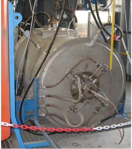
The object of the numerical modeling is the gas pre-heating section of IPFR (Isothermal Plug Flow Reactor), which was designed and manufactured in 1994 in Ijmuiden, the Netherlands and belongs to ENEL Ricerca, Livorno, Italy. This facility is an example of advanced equipment for pulverized fuel characterizations (i.e. coal 40-150 µm), in order to identify TAR and CHAR concentrations. It is pos-sible to investigate devolatilization and char burnout separately, under conditions that solid fuel particles experience in an industrial flame. The reactor enables the coal to be characterized under a wide variety of residence times, particle heating rates and combustion atmospheres [47]. The IPFR is routinely used to investigate the following aspects:

• Devolatilization characteristics of solid fuels and their blends 1_{L.Pietrasanta a.a.2010-2011}

(2)

Chapter 3. Prediction of NO emissions in a pilot-scale burner

• Burnout and combustion rates of various chars • Ignition properties of solid fuels and blends • Ash properties

• Slagging

• Nitrogen chemistry – fate of fuel nitrogen

Fuel particles are injected into a well-defined combustion environment and collected after a residence time in the reactor between 5 to 1500 ms.

IFRF Report N G03/y/03 Description of the Isothermal Plug Flow Reactor Livorno, November 2010

5

3.DESCRIPTION OF THE EXPERIMENTAL EQUIPMENT

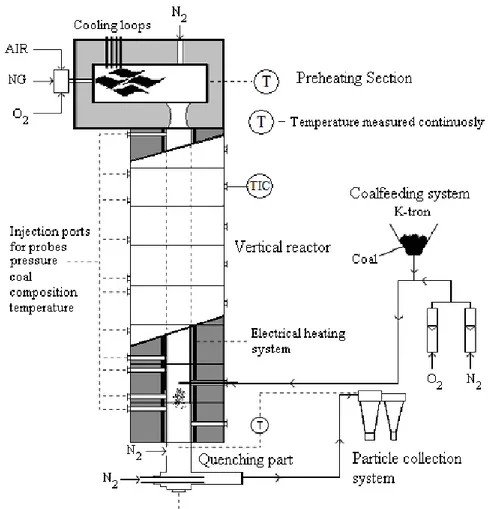
The diagram of IPFR 2008 design is shown in Figure 2 and its characteristics are presented in

Table1. The facility mainly consists of three sections:

! Gas pre - heating section,

! Vertical Isothermal Plug Flow reactor, ! Exhaust line with particle collection system.

Figure 2. Scheme and characteristics of the new asset of the IPFR.

For combustion related studies on solid fuels, it is a drop tube with particles (of the parent fuel or its char) fed pneumatically at a certain height due to the presence of different ports along the tube. The heating is provided by electrical resistances along the tube as well as hot gases from the burner at

Figure 3.1: Scheme and characteristics of IPFR facility

The facility mainly consists of three sections (Figure 3.1): • Gas pre-heating section.

• Vertical Isothermal Plug Flow reactor: the reactor tube consists of eight modules which can be independently controlled and heated electrically with silicon carbide U-type heating elements. Each module is 500 mm height and

(3)

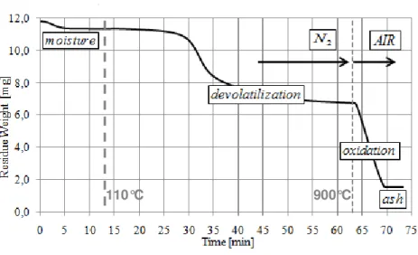
has several ports for accessing diagnostic or feeding devices, three ports for the first two modules and two for the other six. In this way isothermal con-ditions can be obtained within a margin of 10� along the reactor tube in the temperature range of 700 to 1400�. The pulverized fuel coming from the coal feeding system is transported by air, nitrogen or nitrogen-oxygen mixtures to reproduce the oxygen concentration in the flue gases. In this section de-volatilization, gasification, combustion, reduction and solid defragmentation occur (Figure 3.2). Volatiles are released (TAR) and char is produced. The former are burnt immediately, while the latter is burnt in a longer time and carbon residue depends only on the residence time inside the reactor, which can be regulated varying air, gas or flue gas mass flow.

• Exhaust line with particle collection system: the sampling probe is inserted from the bottom of the reactor in order to collect part of the gas-solid mixture. Gas flow rate and cooling system are designed to guarantee that the gas inside the probe has a temperature low enough to stop the combustion reactions. Also a nitrogen quench is available to stop the oxidation reactions in the probe. Estimating carbon residue weight and the residence time inside the reactor, it is possible to define CHAR characteristics.

IFRF Report N G03/y/03 Description of the Isothermal Plug Flow Reactor

Livorno, November 2010

27 Figure 21. Weight loss curve during the thermogravimetric analysis

Table 4. TG reactivity parameters

Parameter Definition

Units

T

0.05

Temperature at which the conversion is 5%

°C

T

onset

Onset temperature: intersection of tangents at the first weight

loss step

°C

T

peak

Peak temperature: temperature at which the reaction rate is

maximum

°C

R

max

Maximum reaction rate (absolute value)

s

-1

x

Tpeak

Conversion at the peak temperature

-

T

offset

Offset temperature: intersection of tangents at the last weight loss °C

T

0.95

Temperature at which the conversion is 95%

°C

Proximate and TG analysis are used to estimate the conversion after the IPFR runs. In particular the

ash content of parent fuel and solid residue must be evaluated on a dry basis. The conversion is

determined after devolatilization and char oxidation IPFR tests with the ash tracer method. The

following formulas are used:

100

1

0

⋅













−

=

ash

X

for devolatilization tests

110°C 900°C

Figure 3.2: Weight loss curve during the thermogravimetric analysis

3.1.1 Gas Pre-Heating Section

The gas preheating section supplies the reactor with gases of a desired composition and temperature. This section consists in a natural gas burner of one meter length with an internal diameter of 300 mm, which is the object of this thesis work. The

(4)

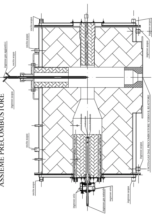
burner (30 kW nominal power) provides hot primary gas in the temperature range from 700 to 1400 �. Flue gases can be mixed with additional gases like nitrogen and carbon dioxide in order to adjust the desired gas composition flow going through the reactor tube. A series of four cooling loops to extract heat from the primary gas flow around the natural gas burner is available. The flue gas temperature can be also adjusted through the injection of ambient temperature nitrogen. Others details are reported in Figures 3.3 and 3.4 from which geometric data have been taken.

Figure 3.3: Gas pre-heating section

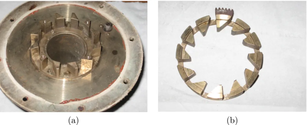
A small air collector (Figure 3.5) is placed at the head of the burner, on which are linked the air pipes destined to cross the swirl, assume tangential motion and get to combustion chamber as primary air, in order to create a recirculation zone for flame stabilization. The air collector have four radial inputs and is made up of a stationary-moving swirl system driven by a shaft built on a ring nut, which allows to modify swirl conditions (Figure 3.6). The external pipes are designed for secondary air flux (Figure 3.7). Instead, the fuel is fed coaxially to the primary air flux and it is injected into the combustion chamber through a central probe.

(5)

Figure 3.4: Gas pre-heating section 2

(6)

(a) (b)

Figure 3.5: Air collector, external (a) and internal (b) view.

(a) (b)

Figure 3.6: Swirl system, fixed (a) and moving (b) parts.

3.1.2 Experimental campaign n.1

The experimental campaign n.1 was carried out in April 2011 in IFRF/Enel Ricerca. The gas pre-heating section was fed with the NG-Air mixture shown in Table 3.1, while NG composition is pointed out in Table 3.2. In these tests swirl inlets were completely open, so no partialization occurred. Basing on the flow rates above-mentioned, NG is burnt with a 21.8% excess air ( = 0.81).

Two ODC (Optical Diagnostic of Combustion) [48] probes were used to monitor the progression of combustion, in order to have an axial and a radial perspective of the burner (Figure 3.8). For further details see L.Pietrasanta a.a. 2010-2011.

Table 3.1: Combustion Conditions

Specie ˙Q (Nm3_/h) _{˙m (kg/h) Temperature (K)}

Natural Gas 2.30 1.68 294

Air 27.00 36.35 300

(7)

49 Come si può notare dalla Figura 3.3, il corpo del bruciatore è costituito da refrattario, ricoperto per circa 2/3 da acciaio; in testa è posto un cassonetto d’aria al quale arrivano i condotti dell’aria destinata ad attraversare lo swirl per entrare in camera di combustione come aria primaria. I condotti più esterni sono quelli destinati al flusso d’aria secondario.

Figura 3.3: Corpo del bruciatore

Si può in oltre notare la lancia d’ingresso del gas, ed il posizionamento dei fori dell’aria secondaria in Figura 3.4.

Figura 3.4: Parte del bruciatore affacciata in camera di combustione

(a)

49 Come si può notare dalla Figura 3.3, il corpo del bruciatore è costituito da refrattario, ricoperto per

circa 2/3 da acciaio; in testa è posto un cassonetto d’aria al quale arrivano i condotti dell’aria

destinata ad attraversare lo swirl per entrare in camera di combustione come aria primaria. I

condotti più esterni sono quelli destinati al flusso d’aria secondario.

Si può in oltre notare la lancia d’ingresso del gas, ed il posizionamento dei fori dell’aria secondaria

in Figura 3.4.

(b)

49 Come si può notare dalla Figura 3.3, il corpo del bruciatore è costituito da refrattario, ricoperto per

circa 2/3 da acciaio; in testa è posto un cassonetto d’aria al quale arrivano i condotti dell’aria

destinata ad attraversare lo swirl per entrare in camera di combustione come aria primaria. I

condotti più esterni sono quelli destinati al flusso d’aria secondario.

Si può in oltre notare la lancia d’ingresso del gas, ed il posizionamento dei fori dell’aria secondaria

in Figura 3.4.

(c)

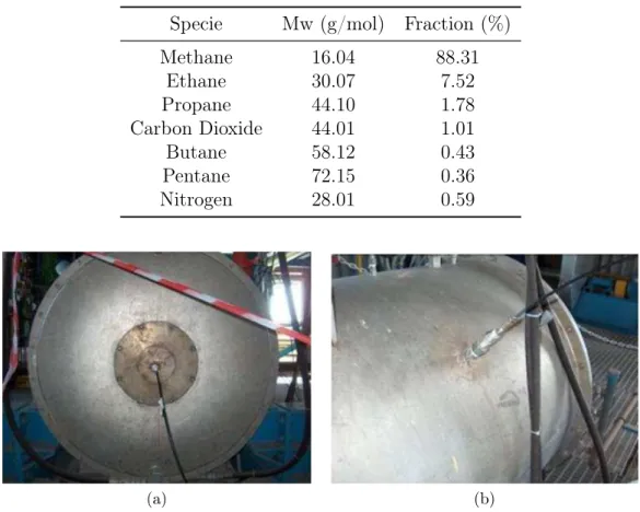
Figure 3.7: Burner body (a-b) and Combustion chamber side (c).

(8)

Chapter 3. Prediction of NO emissions in a pilot-scale burner Table 3.2: Natural Gas Composition, expressed as volume fraction.

Specie Mw (g/mol) Fraction (%)

Methane 16.04 88.31 Ethane 30.07 7.52 Propane 44.10 1.78 Carbon Dioxide 44.01 1.01 Butane 58.12 0.43 Pentane 72.15 0.36 Nitrogen 28.01 0.59

56 con lo strato sottile in cui avviene la reazione della combustione. Quanto supposto implica

l’esistenza di una coerenza tra la componente dinamica dell’emissione radiante e quella della

fluidodinamica turbolenta che può essere messa in evidenza comparando gli spettri che si

ottengono analizzando i segnali forniti da un sistema ODC e da un sistema LDA (anemometria

laser doppler) in grado di fornire lo spettro della fluttuazione della velocità assiale, ovvero della

turbolenza dei gas (combusti e non).

Lo scopo della dislocazione delle sonde è osservare:

- l'integrale delle fluttuazioni radiative della combustione, sonda assiale;

- le fluttuazioni locali della fiamma, sonda radiale (collimata sulla fiamma).

La combinazione delle due informazioni permette di identificare lo stato combustivo:

- La sonda radiale individua la presenza della fiamma e permette di qualificarne tramite

analisi spettrale, lo stato turbolento;

- La sonda assiale verifica la presenza di fiamma lungo tutto l’asse della camera. Avendo

una vista frontale è in grado di rilevare, anche in condizione di combustione mild, la

fiamma che, a causa dell’elevata pressione parziale della miscela comburente/combustibile,

si ha in prossimità del bruciatore.

Figura 3.8: Camera di combustione, posizione sonda assiale e radiale ed angolo di vista

In Figura 3.9, vengono riportati gli andamenti delle variabili di processo con cui si è gestito il

combustore IPFR per passare dalla condizione di combustione in regime flame a quella in regime

flameless e viceversa, e dalla quale è ben visibile l’individuazione delle due fasi transitorie.

(a)

56 con lo strato sottile in cui avviene la reazione della combustione. Quanto supposto implica l’esistenza di una coerenza tra la componente dinamica dell’emissione radiante e quella della fluidodinamica turbolenta che può essere messa in evidenza comparando gli spettri che si ottengono analizzando i segnali forniti da un sistema ODC e da un sistema LDA (anemometria laser doppler) in grado di fornire lo spettro della fluttuazione della velocità assiale, ovvero della turbolenza dei gas (combusti e non).

Lo scopo della dislocazione delle sonde è osservare:

- l'integrale delle fluttuazioni radiative della combustione, sonda assiale; - le fluttuazioni locali della fiamma, sonda radiale (collimata sulla fiamma). La combinazione delle due informazioni permette di identificare lo stato combustivo:

- La sonda radiale individua la presenza della fiamma e permette di qualificarne tramite analisi spettrale, lo stato turbolento;

- La sonda assiale verifica la presenza di fiamma lungo tutto l’asse della camera. Avendo una vista frontale è in grado di rilevare, anche in condizione di combustione mild, la fiamma che, a causa dell’elevata pressione parziale della miscela comburente/combustibile, si ha in prossimità del bruciatore.

Figura 3.8: Camera di combustione, posizione sonda assiale e radiale ed angolo di vista

In Figura 3.9, vengono riportati gli andamenti delle variabili di processo con cui si è gestito il combustore IPFR per passare dalla condizione di combustione in regime flame a quella in regime

flameless e viceversa, e dalla quale è ben visibile l’individuazione delle due fasi transitorie.

(b)

Figure 3.8: Axial (a) and radial (b) probe.

Figure 3.9 shows the radial temperature profile measured by the radial probe at axial coordinate x = 122 mm from the inlet section. On the other hand, the axial probe measured an outlet temperature of 1100 �.

3.1.3 Experimental campaign n.2

The experimental campaign n.2 was carried out in April 2013 in IFRF/Enel Ricerca. These tests [49] were focused to check the reliability and the eﬀectiveness of a new method of spectra analysis. The gas pre-heating section was fed with a NG/air mix-ture with addition of a 0.88 M ammonia solution (Table 3.3). The measurements were made through a measurement equipment called FTIR (Fourier Transform In-fraRed Spectroscopy) analyser at the red points shown in Figure 3.10. They are at the exit of the burner and in two radial position along axial coordinate x = 122 mm: on the flame axis and on the flame border (to 100 mm from the flame axis). The ammonia solution was added to the natural gas using a Gilson dispenser (Figure 3.11).

(9)

Species concentration Temperature

1478 1523 1628 1680 1628 1523 1478 The-X/axis-is-aligned-with-the-points-of-measurement.-The-Y/axis-is-aligned-with-the-axis-of-the-burner.

Comparison between conventional and oxy-fuel combustion Oxy-fuel combustion Conventional combustion 0%- 2%- 4%- 6%- 8%- 10%- 12%- 14%-/150- /100- /50- 0- 50- 100- 150-Co nc en tr a) on *%v ol *d ry * Posi)on*[mm*from*the*centre]* O2- CO2- 0%- 2%- 4%- 6%- 8%- 10%- 12%- 0%- 10%- 20%- 30%- 40%- 50%- 60%- 70%- 80%- 90%- 100%-/150- /100- /50- 0- 50- 100- 150-Co nc en tr a) on *O 2* %v ol dr y* Co nc en tr a) on *C O 2* %v ol *d ry * Posi)on*[mm*from*the*centre]* C O2- 60%- 65%- 70%- 75%- 80%- 85%- 90%- 95%- 10 0%- 2%- 4%- 6%- 8%- 10%- 12%-/150- /100- /50- 0- 50- 100- 150-CO 2* ox y* co nc *%v ol *d ry * O 2, *C O 2* & *O 2* ox y* co nc *%v ol *d ry * Posi)on*[mm*from*the*centre]* O2- CO2-O2-oxy- CO2-oxy- 1400- 1450- 1500- 1550- 1600- 1650- 1700- 1750- 1800-/150- /100- /50- 0- 50- 100- 150-Temp eratu re*( K) * Posi)on*[mm*from*the*centre]*

Figure 3.9: Radial temperature profile at x = 122 mm

3.1.3.1 FTIR System Description

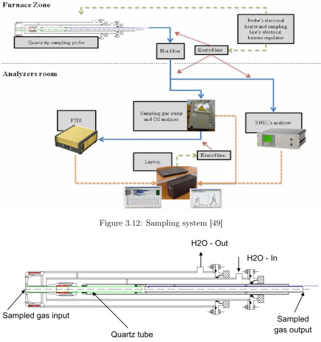
The sampling line [49] (Figure 3.12) is designed to sample the gases in the com-bustion chamber and deliver them to the analyser as much unaltered as possible. To achieve this objective it is necessary to cool down the gases below 300� to avoid water condensation until they reach the analyser. In fact, a small amount of condensation water could reduce considerably the concentration of NH3 and HCN.

The main components of sampling line are listed below.

Sampling probe (Figure 3.13) The material of the tip of the inner tube where the gases are sampled from the furnace is quartz, in order to avoid unwanted reactions between NO and stainless steel. In this region the sampled gases are cooled down below 300� and flow through an electrical heated tube in order to keep temperature constantly higher than 150� to avoid condensation.

(10)

Table 3.3: Summary of the experimental campaign n.2 [49]

Run ˙QN G(N m3/h) ˙QAir(N m3/h) ˙mN H3(g/h) 1 2.30 27.00 0 2 2.30 27.00 48.0 3 2.30 27.00 147.3 4 2.30 27.00 252.5 5 2.30 27.00 335.6 6 2.30 27.00 450.0

IFRF Doc N. F/xx/y/xx Research Report

Livorno, April 2013 Technique developments

!

Figure 58 Pre-heating section

Figure 59 NH3 solution and natural gas feeding probe

Burner

Flame border

Flame axis Flue gas

Figure 3.10: Measurement points

!

6!holes!for!NG!

NH3!solution!

NG! NH3!solution!

Figure 3.11: NH3 solution and natural gas feeding probe

(11)

IFRF Doc N. F/xx/y/xx Research Report Livorno, April 2013 FTIR SYSTEM DESCRIPTION

14

4 FTIR SYSTEM DESCRIPTION

4.1 Sampling line

The sampling line is designed to sample the gases in the combustion chamber and deliver them to the analyser as much unaltered as possible. In this way the concentrations measured are representative of the concentration of the gases in the sampling point inside the combustion chamber. To achieve this objective it is necessary to cool down the sampled gases below 300°C in few milliseconds to stop the combustion reactions and to maintain their temperature over 150°C to avoid water condensation until they reach the analysers (@@@@@measurements in flame@@@). In addiction the inner part of the probe tip was made of quartz to reduce the reactions of NO with steel when the gases are still hot (@@@@@nitrogen species sampling@@@@).

The sampled gases flow from the exit of the probe (described in par. 4.1.1) through a heated line to a hot filter, and then they are split in two parallel lines that go to the O2 analyser and to

the FTIR. The temperature of the line is measured by thermocouples and controlled by a PC. The heating of the suction line is critical because a small amount of condensed water could reduce considerably the concentration of NH3 and HCN. Hence there must be a lot of

attention to every section and there must not be any cold spot.

In Figure 6Errore. L'origine riferimento non è stata trovata. a scheme of the heated line and of all the connection of the system is shown.

Figure 6 Connections scheme of the sampling system

The main components of sampling line are the following:

Figure 3.12: Sampling system [49]

Livorno, April 2013 FTIR SYSTEM DESCRIPTION

16

The main structure of the probe is made by four AISI 316 stainless steel concentric tubes, the tip (green in Figure 7) of the sampling line is a quartz tube.

Figure 8 shows the details of the probe’s head (enlarged) and of the cooling water flows.

Figure 8 Probe details: water cooling

Moving axially the inner tube (red circle in Figure 8), the length of water cooled quartz section is modified so that different temperature of the gases at the exit of the quartz section can be obtained. H2O - In H2O - Out Sampled gas output Quartz tube

Sampled gas input

Figure 7 Scheme of the nitrogen species sampling probe Figure 3.13: Scheme of the sampling probe [49]

ORION HSS-3000 Hot-Box It is a transportable system designed to supply the sampled gases to the FTIR sensor. The box includes gas sampling pump with a needle valve and a dust filter, the oxygen sensor BUHLER BA 1000, a three way solenoid valve (to separate gas analysis from purge gas) and four temperature regulators.

FTIR analyser Fourier Transform InfraRed (FTIR) Spectroscopy is based on the absorption of an IR beam by the sample gas molecules, which induces vi-brational state changes for each molecule at specific wavelength. The principal components are shown in Figure 3.14. A parallel polychromatic radiation, emitted by IR source, is directed to an interferometer. At the exit, the modulated beam

(12)

is reflected through the gas sample cell and detected by a detector. The result-ing signal is digitized and Fourier transformed by the computer resultresult-ing in a IR spectrum of the sample gas.

19

4.2 FT-IR analyser

4.2.1 Components of a Fourier Transform Infrared Spectrometer

Figure 10 shows the principal components of a typical non-dispersive FTIR spectrometers. A parallel polychromatic radiation from an IR source is directed to an interferometer. The modulated bean is reflected through the gas sample cell. Finally, the detector detects the intensity of the infrared beam. The detected signal is digitized and Fourier transformed by the computer resulting in an IR spectrum of the sample gas.

The unique part of an FTIR spectrometer is the interferometer. Figure 11 shows a Michelson type interferometer. The Michelson interferometer is a good example of the working principles of this kind of instruments.

A mirror collects and collimates the infrared radiation from the source before it strikes the beam splitter. The beam splitter ideally transmits one-half of the radiation, and reflects the other half. Both transmitted and reflected beams strike plane mirrors, which reflect the two beams back to the beam splitter. Thus, one-half of the infrared radiation that finally goes to the sample gas has first beam reflected from the beam splitter onto the moving mirror, and then back to the beam splitter. The other half of the infrared radiation going to the sample gas has first gone through the beam splitter and then reflected from the fixed mirror back onto the beam splitter. When these two beams from two optical paths are reunited, interference occurs at the beam splitter. The strength of the interference is depended on the optical path difference between the beams caused by the position of the moving mirror.

Source

Beamsplitter

Radiation2to2the2sample2gas2and2detector Moving2mirror

Fixed2mirror

Figure 11 Michelson interferometer

Infrared source

Interferometer Detector Signal and data

processing unit Sample

cell

Figure 10 The basic components of an FTIR spectrometer

Figure 3.14: Basic component of a FTIR spectrometer [49]

The major diﬀerence between a FTIR and a dispersive IR spectrometer is the Michelson Interferometer (Figure 3.15). It consists of two perpendicular mirrors (one stationary and one movable) and a beam-splitter, which ideally transmits one-half of the radiation, and reflects the other one-half. Subsequently, both transmitted and reflected beams strike plane mirrors and are reflected back to the beam-splitter. If the distances travelled by two beams are the same, which means the distances between two mirrors and the beam-splitter are the same, the situation is defined as zero path diﬀerence (ZPD). If the movable mirror moves away from the

beam-IFRF Doc N. F/xx/y/xx Research Report

19 4.2 FT-IR analyser

4.2.1 Components of a Fourier Transform Infrared Spectrometer

Figure 10 shows the principal components of a typical non-dispersive FTIR spectrometers. A

parallel polychromatic radiation from an IR source is directed to an interferometer. The

modulated bean is reflected through the gas sample cell. Finally, the detector detects the

intensity of the infrared beam. The detected signal is digitized and Fourier transformed by the

computer resulting in an IR spectrum of the sample gas.

The unique part of an FTIR spectrometer is the interferometer. Figure 11 shows a Michelson

type interferometer. The Michelson interferometer is a good example of the working

principles of this kind of instruments.

A mirror collects and collimates the infrared radiation from the source before it strikes the

beam splitter. The beam splitter ideally transmits one-half of the radiation, and reflects the

other half. Both transmitted and reflected beams strike plane mirrors, which reflect the two

beams back to the beam splitter. Thus, one-half of the infrared radiation that finally goes to

the sample gas has first beam reflected from the beam splitter onto the moving mirror, and

then back to the beam splitter. The other half of the infrared radiation going to the sample gas

has first gone through the beam splitter and then reflected from the fixed mirror back onto the

beam splitter. When these two beams from two optical paths are reunited, interference occurs

at the beam splitter. The strength of the interference is depended on the optical path

difference between the beams caused by the position of the moving mirror.

Source

Beamsplitter

Radiation2to2the2sample2gas2and2detector Moving2mirror

Fixed2mirror

Figure 11 Michelson interferometer

Infrared

source

Interferometer

Detector

Signal and data

processing unit

Sample

cell

Figure 10 The basic components of an FTIR spectrometer

Figure 3.15: Michelson interferometer [49]

splitter, the light beam, which strikes the movable mirror, will travel a longer distance. When these two beams from two optical paths are reunited, interference occurs at the beam splitter. The diﬀerence between the two optical path length is known as the retardation. An interferogram is obtained recording the signal from the detector for various values of the retardation. The form of the interferogram, when no sample is present, depends on factors such as the variation of source in-tensity and splitter eﬃciency with wavelength. This results in a maximum when waves are in phase (zero retardation) and minimum when waves are in phase op-position. When a sample is present, the background interferogram is modulated

(13)

by the presence of absorption bands in the sample.

For each wavelength, the gas transmittance coeﬃcient ⌧ is the intensity of the IR radiation that has passed through the sample gas (I) divided by the intensity of the IR radiation that has entered the sample gas (I0).

⌧ = I

I0 (3.1)

while the absorbance A is:

A = log10

1

T (3.2)

Beer’s law (3.3) is the basic law for spectroscopic quantitative analysis. It shows how the concentration of sample gas is related to the measured absorbance of the sample spectrum:

A = log10

I0

I = abc (3.3)

In the above equation a is the absorptivity, that is the capacity of the molecule to absorb IR radiation, b is the optical path length, that is the distance traversed by the IR radiation beam in the gas sample. The quantity c indicates the concen-tration of gas molecules in the sample, so, if the optical path length is constant, Beer’s law states that the absorbance is directly proportional to the concentration of the sample gas at a given wavelength. For the additivity of the law, the total absorbance is equal to the sum of the single values of each gas component. The de-gree of absorption of IR radiation at each wavelength relates quantitatively to the number of absorbing molecules in the sample gas. Since there is a linear relation-ship between the absorbance and the number of absorbing molecules, quantitative multi-component analysis of gas mixtures is feasible.

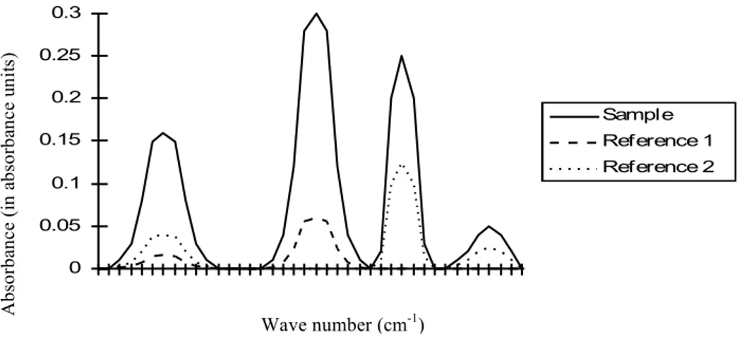
To perform multi-component analysis it is required to have the sample spectrum and the reference spectra of all the gas components that may be present. In multi-component analysis, the objective is to combine these reference spectra with appropriate multipliers in order to get a spectrum that is as close as possible to the sample spectrum. If this happens, the concentration of each gas component can be evaluated using the multipliers of the individual reference spectra, known the concentration of the reference gases.

It is possible to use Figure 3.16 as an example. In this case, it is assumed to be known that the sample gas consists of gases Reference 1 and Reference 2. The reference spectra available represent concentrations of 10 ppm and 8 ppm, respectively. To find out the real concentration of each component in the sample gas, the measured sample spectrum must be reproduced using a linear combination of the two reference spectra. Multiplying the spectrum Reference 1 by 5 and the

(14)

spectrum Reference 2 by 2, and combining these two spectra it is possible to get a spectrum that is similar to the sample one. So, the concentrations of gases Reference 1 and Reference 2 are 50 and 16 ppm, respectively.

IFRF Doc N. F/xx/y/xx Research Report Livorno, April 2013 FTIR SYSTEM DESCRIPTION

24

Multi-component analysis

The degree of absorption of infrared radiation at each wavelength relates quantitatively to the number of absorbing molecules in the sample gas. Since there is a linear relationship between the absorbance and the number of absorbing molecules, quantitative multi-component analysis of gas mixtures is feasible.

To perform multi-component analysis it is required to have the sample spectrum and the reference spectra of all the gas components that may be present in the sample. A reference spectrum is a spectrum of one single gas component of specific concentration. In multi-component analysis, the objective is to combine these reference spectra with appropriate multipliers in order to get a spectrum that is as close as possible to the sample spectrum. If the analysis succeeds in forming a spectrum similar to the sample spectrum, then the concentration of each gas component in the sample gas can be evaluated using the multipliers of the individual reference spectra, known the concentration of the reference gases.

Figure 13 An example of spectra for multi-component analysis

The sample spectrum and reference spectra shown in Figure 13 can be used as an example. In this case, it is assumed to be known that the sample gas consists of gases Reference 1 and Reference 2. The reference spectra available represent concentrations of 10 ppm and 8 ppm, respectively. To find out the concentration of each component in the sample gas, the measured sample spectrum must be reproduced using a linear combination of the two reference spectra. Multiplying the spectrum Reference 1 by 5 and the spectrum Reference 2 by 2, and combining these two spectra it is possible to get a spectrum that is similar to the sample one. Accordingly, the sample gas contains reference gas 1 at five times the amount in the reference spectrum 1, and reference gas 2 at two times the amount in the reference spectrum 2. The analysis indicates that the sample indeed consists of these two reference gases. The concentration of the reference gas 1 in the sample is found to be 50 ppm (5x10ppm), and the concentration of the reference gas 2 in the sample is 16 ppm (2x8ppm). A more complex case is shown in Figure 14.

0 0.05 0.1 0.15 0.2 0.25 0.3 Sample Reference 1 Reference 2 Ab so rb an ce (i n ab so rb an ce u ni ts ) Wave number (cm-1₎

Figure 3.16: Example of multi-component analysis [49]

The FTIR analyser used during this campaign is the Gasmet™ DX4000, which is connected to a laptop, in order to acquire data. On it, a software called Calcmet™ was installed, which analyses the sample spectrum using sophisticated and patent protected multicomponent algorithms. It is capable of simultaneous detection, identification, and quantification of up to 50 diﬀerent gas components, such as H2O, CO, CO2, NO, NO2, N2O, NH3, HCl, HF, CH4 and diﬀerent VOC’s2.

The sequence to analyse correctly a sample is the following: • Select the components that will be analysed.

• Measure the background with the sample cell filled with a zero gas, such as nitrogen, which does not absorb IR radiation.

• Measure and analyse the sample. The measurement time can vary on the range 1 s - 1 min. The smaller the concentrations measured are, the longer the measurement time should be.

• Verify the results. The residual between the measured sample spectrum and the model used in the analysis for the selected component is usually taken as convergence indicator. If the residual does not show any clear peaks but noise, the analysis was successful. On the contrary if there are significant spectral peaks on any areas that are used for analysis or the base line is tilted, there is possibly some unknown component present, something wrong in the analysis settings, or some components out of calibrated range.

2_{Volatile Organic Compounds}

(15)

• The analysis results are based on the reference spectra that were selected for the analysis. The concentration are calculated by comparing the sample spectrum to the reference spectra. The absolute amounts and units depend on the conditions (concentration, path length, etc.) at which the reference spectra are recorder. Thus, the accuracy of the analysis results can only be as good as the accuracy of the reference spectra.

3.2 Numerical modeling

The present Section reports the choices adopted in the numerical modeling of the gas pre-heating section. The approach was varied during the development of this thesis, depending especially on the operating condition (NG/air or NG/NH3/air).

The mathematical modeling has been carried out with the commercial code Fluent by Ansys Inc.

3.2.1 Computational domain and grid

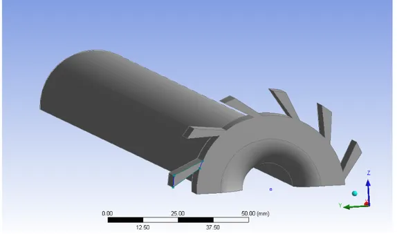
The computational domain consists of two sub-domains: the swirl duct and the combustion chamber. The profile (three components of velocity, turbulence kinetic energy (k), dissipation rate (!) or specific dissipation rate (✏)) at the exit of the former was used as an input for the latter. In both cases, due to the periodicity of the geometry, only a 180 degrees angular sector was modeled through Ansys Workbench (Figures 3.17 and 3.18), in order to reduce the number of cells. The secondary air and fuel ducts were extended upstream to ensure the flow to be fully developed at the burner inlet.

Swirl Duct Due to the geometric simplicity and the absence of local higher resolution, the 3D grid, built with the software ICEM CFD, is structured and consists of around 356k hexahedrons (Figure 3.19).

Combustion Chamber A set of four 3D grids with a number of cells ranging from 400k to 1.600k were firstly built with the software Gambit and investigated. Each of them contains parts meshed with tetras (near inlet jets) and parts with hexahedrons (burner body and outlet). The choice of a hybrid grid is justified to reduce the number of cells required to define the computational domain accurately, as a grid constituted only of tetras would require a huge amount of cells. Although it was not possible to perform a classic Richardson extrapolation, being the grid spacing non-uniform using a hybrid grid, the values of diﬀerent output variables,

(16)

Figure 3.17: Swirl geometry

!

Secondary!Air!

Primary!Air!

3!Fuel!Jets! Ammonia!Jet!

Figure 3.18: Burner geometry

(17)

!

Figure 3.19: Swirl domain grid

i.e. temperature and axial veloctiy, were monitored to guide the selection of the computational grid. In this way, the selected grid consists of 800k cells (Figure 3.20).

Unfortunately, it was noticed that all the grid built were not sufficient fine to predict the flame front properly, in fact a big numerical diffusivity effect was introduced, leading the flame to be attached to the walls, as shown in Figure 3.21. Thus, a higher resolution in the first part of the burner (near inlet jets) was needed. To achieve this object it was used the Size Function modality of Gambit [50], which allows to control the size of the mesh in regions surrounding a specified entity. It is similar to boundary layers in that they control the mesh characteristics in the proximity of the entities to which it is attached. To define a size function, it is important to specify the source, that is the center of the region in which the size function applies, and the attachment, that is the entity for which the mesh is to be affected by the size function. Each individual size function is associated with only one source but may be associated with one or more attachment entity.

Finally, the selected grid (Figure 3.22) consists of around 1.900k cells, 1.550k tetras and 350k hexahedrons. In this way, more than 1.000k cells are focused in the conical region, near the jets.

(18)

(a) (b)

(c)

Figure 3.20: Burner domain, grid 800k cells

3.2.2 Boundary Conditions

The resolution of the discretized form of the Navier-Stokes equations requires the attribution of boundary conditions at the domain boundary. The definition of the boundary condition types have to be made after meshing the domain in the software Gambit or ICEM, while the setting of the quantities to be assigned at each boundary condition is directly implemented in the Fluent code.

At the fuel inlet, the mass flow with its composition and temperature was specified. Concerning this, the composition of natural gas (NG) was simplified firstly as pure CH4and later as a CH4/C2H6(91.4%-9.6% as mass fraction) mixture.

Moreover, NG is fed at ambient temperature (a value of 298 K was assumed). The primary air inlet was set as velocity inlet and the profiles of x-y-z velocity, turbulence kinetic energy, dissipation or specific dissipation rate were taken from

(19)

Figure 3.21: Contours of Temperature (800k cells)

the exit of the swirl. At the outlet section the relative pressure was assigned. Since the burner operate at atmospheric pressure, the value was set to zero.

Particular attention was paid to the walls. In fact, the walls in the inlet re-gion were set as adiabatic, while for the lateral walls composing the burner body were used two diﬀerent boundary conditions. It was firstly set the heat flux ex-changed with the external cooling loops, which can be estimated in the following way. Considering a multicomponent system undergoing chemical reactions, the first principle can be written as:

Q + W = X P NPh¯P X R NRh¯R (3.4)

where P and R indicate the products and reactants, respectively. Moreover, the enthalpy of the ith _{species at condition (T,p) can be defined as:}

¯

hi(T ) = ¯hf,i 0

+ hi(T ) (3.5)

where hf,i0 is the heat released or absorbed during the formation of the ith species

from its elements. We assume that the enthalpies of formation are zero for the elements in their naturally occurring state at the reference state temperature and pressure (298 K and 110 kPa). Considering the variation of enthalpy with temper-ature, equation (3.5) can be written as:

¯ hi(T ) = ¯hf,i 0 + Z Tout Tref ¯ cp,idT (3.6) 55

(20)

(a) (b)

(c)

Figure 3.22: Burner domain, grid 1.900k cells

The value of Tout is taken from experimental campaign n.1 (1373 K). Thus, the

heat flux exchanged can be written as:

Q =X P ⌫P ✓ ¯ hf,i 0 + Z Tout Tref ¯ cp,idT ◆ P X R ⌫R ✓ ¯ hf,i 0 + Z Tout Tref ¯ cp,idT ◆ R (3.7)

Subsequently, for problems of convergence, a boundary condition of the first kind was set, imposing the value of temperature obtained in experiment campaign n.1 at the wall (r = 150 mm), that is 1478 K.

For what concern experiment campaign n.2, the same boundary conditions were applied, except for the ammonia solution injection, where diﬀerent values of mass flows were set.

(21)

3.2.3 Turbulence Model

Combustion processes in many practical system take place within turbulent flow regimes, so they are diﬃcult to predict. In fact, turbulent combustion results from a two way interaction between chemistry and turbulence: when a flame in-teracts with a turbulent flow, turbulence is modified by combustion because of the strong accelerations through the flame front induced by heat release, and because of the large changes in density and kinematic viscosity associated with tempera-ture changes. This mechanism may generate turbulence or damp it. On the other hand, turbulence alters the flame structure: it may enhance chemical reactions but it could also lead to flame quenching, when the turbulent mixing is too intense.

The direct numerical simulation of the instantaneous balance equations is not possible for practical combustion systems, so to overcome such diﬃculty, the bal-ance equations are averaged to describe only the mean flow field with a RANS approach, using diﬀerent turbulence models to evaluate the Reynolds stress ten-sor. Moreover, in order to consider the large changes in the fluid density typical of combustion process, the Navier-Stokes equations have been averaged by means of the Favre definition (Favre-Averaged Navier Stokes, FANS).

The two-equation turbulence models tested during the simulations of campaign n.1 and n.2 are listed below.

Standard k-✏ This model, proposed by Launder and Spalding [51], is based on model transport equations for the turbulence kinetic energy (k) and its dissipa-tion rate (✏). The former is derived from the exact equadissipa-tion, while the latter is obtained using empiricism and physical reasoning and bears little resemblance to its mathematically exact counterpart. In fact, the standard constants of ✏ equa-tion come from experiments. Robustness, economy and reasonable accuracy for a wide range of turbulence flows explain the popularity of the standard k-✏ model. Finally, combining k and ✏ is possible to compute the turbulent viscosity µt as

follows, considering Cµ as a constant:

µt= ⇢Cµ

k2

✏ (3.8)

RNG k-✏ The RNG k-✏ model [52] is derived using a statistical technique called renormalization group theory. This analytical derivation results in a model with constants diﬀerent from those in the standard model, and additional terms and functions in the transport equation for k and ✏. In fact, unlike the standard model, it includes the eﬀect of swirl on turbulence and an additional term in its ✏ equation,

(22)

improving the accuracy for swirling and rapidly strained flows. It is also possible to specify an analytical formula for turbulent Prandtl number and to take into account low-Reynolds number eﬀect.

Realizable k-✏ The realizable k-✏ model [52] diﬀers from the standard model because it contains an alternative formulation for the turbulent viscosity and a modified transport equation for the dissipation rate (✏), which is derived from an exact equation on the Reynolds stresses, consistent with the physics of turbulent flows.

Both the realizable and RNG k-✏ models have shown improvements over the standard model, especially where the flow features include strong streamlines.

Standard k-! This model, firstly proposed by Kolmogorov [53] and improved by Wilcox [54], is an empirical model based on model transport equations for the turbulence kinetic energy (k) and the specific dissipation rate (!). The correlation between the variables is the following:

µt= ⇢

k

! (3.9)

Although the k-! model is not as popular as the k-✏ model, it has several advan-tages, namely that:

• the model is reported to perform better in transitional flows and in flows with adverse pressure gradients;

• the model is numerically very stable, especially the low-Re version, as it tends to produce converged solutions more rapidly than the k-✏ models;

• the low-Re version is more economical and elegant than the low-Re k-✏ mod-els, in that it does not require the calculation of wall distances, additional source terms and/or damping functions based on the friction velocity.

k-! SST Menter [55] in 1992 noted that the near-wall performance of k-✏ model is unsatisfactory for boundary layer with adverse pressure gradient. This led him to suggest a hybrid model using a transformation of the k-✏ model into a k-! model in the near-wall region and the standard k-✏ in the fully turbulent region far from the wall. The Reynolds stress computation and the k-equation are the same as in Wilcox’s k-! model [52], but the ✏-equation is transformed into a !-equation by substituting ✏ = k!. In this way, the model avoids the common k-! problem that the model is too sensitive to the inlet free-stream turbulence properties, but

(23)

otherwise it has a good behaviour in adverse pressure gradients and separating flow.

3.2.4 Turbulence/chemistry interactions and kinetic

mech-anisms

Turbulence/chemistry interactions have been modeled through the choice of the combustion model. In particular, the Eddy Dissipation/Finite Rate (ED/FR) model and the Eddy Dissipation Concept (EDC) have been considered. According to the ED/FR model both a mixing rate and an Arrhenius rate, based on the mean properties, are evaluated and the smallest one is chosen as the mean reaction rate for the reacting species. However, the ED/FR model does not allow to implement detailed kinetic mechanism for gas-phase combustion being the turbulent rate the same for all the reactions.

This is precisely why, subsequently, the Eddy Dissipation Concept (EDC) by Magnussen [44] was taken into account. According to EDC, combustion occurs in the region of flow where the dissipation of turbulence kinetic energy takes place. Such regions are called fine structures and they can be described as homogeneous, pressure-constant reactors. The length fraction of the fine structures is modeled as [52]: ⇠⇤ = C⇠ ⌫✏ k 1/4 (3.10) where C⇠ is a volume fraction constant equal to 2.1377 and ⌫ is the kinematic

viscosity. Species are assumed to react in the fine structures over a time scale:

⌧⇤ = C⌧

⌫ ✏

1/2

(3.11)

where C⌧ is a time scale constant equal to 0.4082. Reactions proceed over the time

scale and the rate of progress for reaction j, Qj, can be expressed as:

Qj = kf j N Y k=1 ✓ ⇢Yk Wk ◆⌫‘ kj krj N Y k=1 ✓ ⇢Yk Wk ◆⌫“ kj (3.12) where ⌫‘

fj and ⌫“fj are the molar stoichiometric coeﬃcients of species k, kfj and krj

are the forward and backward kinetic constants of reaction j, while the bracketed quantity is the molar fraction of species k. The forward kinetic constant is expressed using the so called Arrhenius law:

kf j = Af jT je

Eaj

RT (3.13)

(24)

while reverse constants are derived from equilibrium constants. In order to express the rate of progress Qj for each reaction, data for the pre-exponential factor, Aj,

the temperature exponent, j, and the activation energy, Eaj, must be provided.

The rate of progress of each reaction is integrated numerically using the In Situ Adaptive Tabulation (ISAT) algorithm of Pope [45], which can accelerate the chemistry calculations by two to three orders of magnitude, oﬀering substantial reductions in run-times. In fact, for kinetic mechanisms that are deterministic, the final reacted state is a unique function of the initial unreacted state and the time-step. This reaction mapping can, in theory, be performed once and tabulated. The table can then be interpolated with run-time speed-up as long as interpolation is more eﬃcient than chemistry integration.

In order to simulate experimental campaign n.1, three diﬀerent kinetic mech-anisms have been used to describe the oxidation of NG. Global kinetic rates are applied with the ED/FR model. When using the EDC model, the global reaction approach has been compared to one reduced mechanism, the KEE [43] (in pure methane condition) and one detailed mechanism, the GRI-3.0 [56] (in methane-ethane mixture). The former includes 17 species and 58 reversible chemical re-actions, instead the latter has been implemented without NOx reactions, not to

exceed the maximum number of species transport equations which can be solved by the code, resulting in 219 reversible reactions involving 36 chemical species.

3.2.5 NO

x

formation model and ammonia modeling

On the basis of the work done in Section 2.2 another comprehensive modeling approach for NOx formation has been developed on the specific conditions of

Ex-perimental champaign n.2 (Table 3.4). Once again, the Prompt NO formation is neglected during the development of the model and the main reactions involved in NO formation have been evaluated through a PSR, using Glarborg [19] detailed kinetic scheme. To do that, once again the software OpenSMOKE [41] is needed.

Table 3.4: PSR operating conditions

Parameter Value ˙QN G(N m3/h) 2.30 ˙QAir(N m3/h) 27 ˙mN H3(g/h) 0-450 T(K) 1500-1900 p (atm) 1 ⌧(ms) 480 60

(25)

Rate of production analysis (Figure 3.23) shows that thermal route is the main mechanism forming NOx. HNO and NO2 are significant educts for NO formation,

but completely converted back, as Löﬄer et al. [18] suggest.

Rate of Production Analysis - NO

306 N+NO=N2+O 72557.930 304 N+OH=NO+H 62254.684 240 NO+O+M=NO2+M -33494.429 243 NO2+H=NO+OH 30555.506 305 N+O2=NO+O 16327.269 253 HNO+H=H2+NO 9591.150 255 HNO+OH=NO+H2O 9042.754 338 HCO+NO=HNO+CO -7647.016 238 H+NO+M=HNO+M -7519.389 346 CH+NO=HCO+N -7164.749 293 NH+O=NO+H 3981.596 239 H+NO+N2=HNO+N2 -2834.532 298 NH+NO=N2O+H 2211.986 244 NO2+O=NO+O2 1623.616 242 HO2+NO=NO2+OH 1104.927 254 HNO+O=NO+OH 952.906 319 NNH+O=NH+NO 814.949 300 NH+NO=N2+OH 692.847 299 NH+NO=N2O+H -644.435 329 N2O+O=2NO 623.568

Figure 3.23: NO Rate of production analysis (ROPA). Blue lines indicate NO destruction, while the red ones NO formation

Applying the same hypothesis made in Section 2.2 is possible to evaluate the main reactions involving the intermediate species N, N2O, NO2, NNH, NH, HNO,

HONO, NH2 and, then, their concentrations, which are listed in Appendix C with

the kinetic parameters used.

Ammonia injection has been modeled coupling the present model with a user-defined-scalar (UDS), which has been added to the transport equation for species solved by the code. The former has been implemented by means of a user-defined-function (UDF) and the concentration of NH3 is taken from UDS. On the contrary,

the latter uses the source term expressed in UDF.

3.2.6 Radiation model and radiative properties

The evaluation of the heat source term due to absorbed or emitted radiation ˙Qrad

is of particular importance since the thermal radiation is the main heat transfer in high temperature problems. Obviously, the thermal radiation equation is coupled to energy conservation equation, since temperature is one of the unknown.

(26)

The radiative transfer equation (RTE) can be express as: dI(r, s)

ds = Ib(r) I(r, s) sI(r, s) +

s 4⇡ Z 4⇡ I (s_i) (s_i, s)d⌦i+ SR (3.14) where:

• I(r, s) is the intensity of the radiation emitted at a frequency ⌫, function of the position vector; (r) and direction (s) within a small pencil of rays, travelling thorough a participating medium [55];

• s is the distance by the radiation from its emission to its absorption (path length);

•  and s indicate the absorption and scattering coeﬃcients, respectively;

• Ib is the black body radiation intensity;

• I-(si) is the intensity incident upon the point at r from all possible directions,

si;

• is the scattering phase function, which is defined as the fraction of radiant incident upon the medium along direction vector si, which is subsequently

scattered in direction s; • ⌦ is the solid angle; • SR is a radiation source.

Equation (3.14) is a integro-diﬀerential equation, function of space coordinates, direction, frequency, thus is analytically solvable only for very simple case.

In all the simulation radiative heat transfer equation has been modeled with Discrete Ordinate (DO) model, which solves the RTE equation for a finite number of discrete solid angle. The fineness of the spatial discretization was assigned choos-ing to divide each of the octants of the angular space 4⇡ into solid angles resultchoos-ing in 32 solid angles, for which the RTE is solved. The DO model transform the RTE equation into a transport equation for radiation intensity in the spatial coordinates (x,y,z) and solves for as many transport equations as there are directions s.

The radiative properties of the gaseous mixture have been evaluated using the Weighted Sum of Gray Gases Model (WSGG), which assumes that the radiative properties of a non-gray gas can be obtained as the weighted sum of certain number

(27)

of gray gases contributes. The basic assumption of WSGG model is that the total emissivity over the distance s can be presented as:

✏ =

Ng

X

i=0

ai(T )(1 e kips) (3.15)

where ai is the emissivity weighting factors for the ith fictitious gray gas, the

bracketed quantity is the ith gray gas emissivity, ki is the absorption coeﬃcient of

the ith gray gas, p is the sum of the partial pressures of all absorbing gases and s is the path length. For ai and ki Ansys Fluent uses values obtained from Coppalle

and Vervisch [57] and Smith et al. [46]. The absorption coeﬃcient (ki), for i = 0, is

considered as zero to account for windows in the spectrum between spectral regions of high absorption, while the weighting factor for i = 0 is evaluated from:

a0 = 1 Ng

X

i=0

ai(T ) (3.16)

The temperature dependence of ai can be approximated by any appropriate

func-tion, but the most common approximation is the following polynomial form:

ai = J

X

j=0

bi,jTj 1 (3.17)

where bi,j are the emissivity gas temperature polynomial coeﬃcients.

A summary of the carried out numerical simulations for the experimental cam-paign n.1 and n.2 is listed in Tables 3.5 and 3.6 respectively.

3.3 Results

The present Section describes the results of the numerical modeling of the pre-heating section and the comparison between the computational results and exper-imental data. The presentation of the results will follow the scheme adopted for the description of the experimental campaigns.

3.3.1 Experimental campaign n.1

3.3.1.1 Swirl Duct

Figure 3.24 shows the velocity field along the swirl duct (a) and at its exit (b-c). It is worth noting the radial component of velocity that air assumes passing through

(28)

Chapter 3. Prediction of NO emissions in a pilot-scale burner -T ab le 3. 5: D et ai ls of th e nu m er ica ls im ul at io ns fo r ex per im en ta lca m pa ig n n. 1 N . Fu el T urb . M od el C om b. M od el K in . Sc he m e R ad . M od el Sp ec tra l M od el L at era l w al l B .C . 1 CH 4 k-✏ E D /F R 1-st ep D O W SG G F lu x 2 CH 4 k-✏ re al . E D /F R 1-st ep D O W SG G F lu x 3 CH 4 k-✏ re al . E D C 1-st ep D O W SG G F lu x 4 CH 4 k-✏ re al . E D C 1-st ep D O W SG G T 5 CH 4 k-✏ ED C KEE D O W SGG T 6 CH 4 k-✏ re al . E D C K E E D O W SG G T 7 CH 4 k-✏ re al . E D C K E E D O W SG G F lu x 8 CH 4 k-! ED C KEE D O W SGG T 9 CH 4 k-! SST EDC KEE DO WSGG T 10 CH 4 /C 2 H6 k-! ED C GRI 3 .0 DO WSGG T 11 CH 4 /C 2 H6 k-! SST EDC GRI 3 .0 DO WSGG T T ab le 3. 6: D et ai ls of th e nu m er ica ls im ul at io ns fo r ex per im en ta lca m pa ig n n. 2 N . Fu el T urb . M od el K in . Sc he m e L at era l w al l B .C . N Ox mo del ˙mNH 3 (g/ h ) NH 3 mo del ing 1 CH 4 /C 2 H6 k-! S S T GRI 3 .0 T P r+ N ew M od el 0 UDS 2 CH 4 /C 2 H6 k-! S S T GRI 3 .0 T P r+ N ew M od el 147 .27 UDS 3 CH 4 /C 2 H6 k-! S S T GRI 3 .0 T P r+ N ew M od el 252 .2 UDS 4 CH 4 /C 2 H6 k-! S S T GRI 3 .0 T P r+ N ew M od el 335 .57 UDS -64

(29)

the duct, which is characterised by a swirl number S = 0.76, estimated as follow [58]: S = 2 3 1 di de 3 1 di de 2 ! tan(✓) (3.18)

where ✓ is the swirl vane angle (45 ), di is the hub diameter and de is the outer

diameter of the duct.

(a)

(b) (c)

Figure 3.24: (a) Pathlines along the swirl duct, coloured by velocity magnitude (m/s). Contours of Radial (b) and Axial (c) velocity (m/s) at the swirl exit. k-✏ realizable turbulence model.

(30)

3.3.1.2 Burner

The results of the CFD analysis on the burner are presented and discussed with two main objectives: i) to investigate the eﬀect of turbulence/chemistry interaction models and kinetic mechanism on the results; ii) to examine the eﬀect of turbulence models on the results.

Eﬀect of kinetic mechanisms/combustion model Figure 3.26 shows the contour plot of temperature and axial velocity obtained with diﬀerent turbu-lence/ chemistry interactions models and kinetic mechanisms, considering pure CH4 as fuel. It can be observed how the ED/FR model (a) shows the presence of a

well-defined high temperature region and maximum temperatures close to the adi-abatic flame temperature (2300 K). High axial velocity values can be observed in the recirculating zone (b). If the EDC model with global chemistry is employed (c), the resulting temperature distribution denotes an extension of the reaction zone to a larger portion of the available volume in the burner, but an higher temperature peak. The axial velocity field (d) is diﬀerent, showing a more penetrating cold central jet. However, only when considering the Kee (e-f) kinetic mechanisms, no local peak and a more uniform temperature distribution is observed in the burner. It is also noteworthy that the cold central jet reaches the half of the burner body. Such considerations can be quantitatively confirmed by the analysis of the radial profiles of temperature at axial coordinate x = 122 mm from the inlet section (Figure 3.25). 0 20 40 60 80 100 120 140 160 600 800 1000 1200 1400 1600 1800 2000 2200 2400 r (mm) T (K) ED/FR 1−step EDC 1−step EDC kee Exp

Figure 3.25: Radial profiles of temperature at x = 122 mm predicted by ED/FR with global chemistry, EDC with global chemistry and EDC with Kee. k-✏ realizable turbulence model.

(31)

(a) (b)

(c) (d)

(e) (f)

Figure 3.26: Temperature (K) and Axial velocity (m/s) distribution predicted by (a-b) ED/FR with global chemistry, (c-d) EDC with global chemistry and (e-f) EDC with Kee. k-✏ realizable turbulence model.

(32)

Eﬀect of turbulence model Figure 3.28 shows the contour plot of temperature and axial velocity, obtained with diﬀerent turbulence models, using the Kee kinetic mechanism. It can be observed how the k-! model (a-b) predicts a flame which reach the lateral walls of the burner. Instead, the contour of k-! SST presents a behaviour more in line with the k-✏, as theory suggests, but with a shorter cold central jet. Such considerations can be quantitatively confirmed by the analysis of the radial profiles of temperature at axial coordinate x = 122 mm from the inlet section. Considering Figure 3.27, the k-! model seems to fit better experimental data. 0 20 40 60 80 100 120 140 160 600 800 1000 1200 1400 1600 1800 2000 r (mm) T (K) K−Eps. Real. K−Om. K−Om. SST Exp.

Figure 3.27: Radial profiles of temperature at x = 122 mm predicted by k-!, k-! SST and k-✏ realizable. Kee kinetic mechanism.

Figure 3.30 shows the contour plot of temperature and axial velocity obtained with diﬀerent turbulence models, using the GRI 3.0 kinetic mechanism and con-sidering a CH4/C2H6 mixture as fuel. It can be observed how the k-! model (a-b)

predicts a similar behaviour compared with the previous case, but with an incre-ment of temperature. Instead, the shorter central cold jet in k-! SST allows to fit better experimental data, except for the local peak at r = 60 mm (Figures 3.29).

(33)

(a) (b)

(c) (d)

(e) (f)

Figure 3.28: Temperature (K) and Axial velocity (m/s) distribution predicted by (a-b) k-!, (c-d) k-! SST and (e-f) k-✏ realizable. Kee kinetic mechanism.

(34)

Chapter 3. Prediction of NO emissions in a pilot-scale burner 0 20 40 60 80 100 120 140 160 1200 1300 1400 1500 1600 1700 1800 1900 2000 r (mm) T (K) K−Om. K−Om. SST Exp

Figure 3.29: Radial profiles of temperature at x = 122 mm predicted by k-! and k-! SST. GRI 3.0 kinetic mechanism.

(a) (b)

(c) (d)

Figure 3.30: Temperature (K) and Axial velocity (m/s) distribution predicted by (a-b) k-! and (c-d) k-! SST. GRI 3.0 kinetic mechanism.

(35)

3.3.2 Experimental campaign n.2

This Section describes the results of the numerical modeling of the second experi-mental campaign on the pilot-scale burner. The discussion will be focused on the comparison between predicted and measured concentration of the main species. The three measurement points are described in Section 3.1.3.

Figures 3.31 and 3.32 show the comparison between predicted and measured concentration of CO and C2H4, as a function of ammomia solution mass flow.

Despite the ammonia solution injection at low temperature (300 K) directly in flame, no combustion eﬃciency reduction occurs, as a negligible concentration of these species in flue gas shows. Moreover, the present model tends to underestimate CO and to overestimate C2H4 predictions at flame axis.

! ! ! ! ! ! ! ! ! ! ! 0! 50! 100! 150! 200! 250! 300! 350! 400! 0! 50! 100! 150! 200! 250! 300! 350! Con cen tration *[ppm ]* NH₃*[g/h

]

*

C

₂

H

_4* 'lue!gas!exp! 'lue!gas! 'lame!axis! exp! 'lame!axis! 'lame!border! exp! 'lame!border! 0! 0.5! 1! 1.5! 2! 2.5! 3! 0! 50! 100! 150! 200! 250! 300! 350! Con cen tration *[% ]* NH₃*[g/h]*

CO

*

'lue!gas!exp! 'lue!gas! 'lame!axis! exp! 'lame!axis! 'lame! border!exp! 'lame! border!

Figure 3.31: Predicted and measured CO concentration in three diﬀerent points.

! ! ! ! ! ! ! ! ! ! ! 0! 50! 100! 150! 200! 250! 300! 350! 400! 0! 50! 100! 150! 200! 250! 300! 350! Con cen tration *[ppm ]* NH₃*[g/h

]

*

C

₂

H

_4* 'lue!gas!exp! 'lue!gas! 'lame!axis! exp! 'lame!axis! 'lame!border! exp! 'lame!border! 0! 0.5! 1! 1.5! 2! 2.5! 3! 0! 50! 100! 150! 200! 250! 300! 350! Con cen tration *[% ]* NH₃*[g/h]*

CO

*

'lue!gas!exp! 'lue!gas! 'lame!axis! exp! 'lame!axis! 'lame! border!exp! 'lame! border!

Figure 3.32: Predicted and measured C2H4 concentration in three diﬀerent points.

(36)

The predicted NO concentration in flue gas (Figure 3.33), based on the new comprehensive model, is in good agreement with measurements, except for the case ˙mNH3 = 150 g/h. However, it is possible to notice an overestimation in flame

border, due probably to a diﬀerent flame structure. It is worth noting also that the higher the ammonia solution mass flow, the greater NO emissions become. In fact, according to Section 1.3.2, the mean temperature inside the burner is higher than the narrow range typical of SNCR technique, allowing the conversion of NH3

into NH2 and, subsequently, NO following reactions (1.37) and (1.38).

! 0! 20! 40! 60! 80! 100! 120! 140! 0! 50! 100! 150! 200! 250! 300! 350! Con cen tration *[ppm ]* NH₃*[g/h]*

NO

₂_* 'lue!gas!exp! 'lue!gas! 'lame!axis!exp! 'lame!axis! 'lame!border! exp! 'lame!border! 0! 20! 40! 60! 80! 100! 120! 140! 160! 180! 200! 0! 50! 100! 150! 200! 250! 300! 350! Con cen tration *[ppm ]* NH₃*[g/h]*

NO*

'lue!gas!exp! 'lue!gas! 'lame!axis!exp! 'lame!axis! 'lame!border!exp! 'lame!border!

Figure 3.33: Predicted and measured NO concentration in three diﬀerent points.

Figure 3.34 shows the relative importance of the diﬀerent NO formation routes, in case of no ammonia injection. Thermal mechanism is the major source of NO (59%), considering the high temperature of combustion (above 1700 K), as pointed out in Section 3.2.5. NNH pathway is also relevant (36%), while N2O, HNO,

NO2 and Prompt routes are negligible. The latter is due to the fuel-lean

condi-tions ( = 0.81). 1%# 59%# 2%# 36%# 2%# Prompt# Thermal# N2O# NNH## NO2+HNO#

Figure 3.34: Relative importance of NO formation routes in case of no ammonia injection.

(37)

In Figures 3.35 and 3.36 it is worth noting that in flame axis it is expected a greater formation of NO2 than N2O, while negligible values are expected in flue

gas. ! 0! 20! 40! 60! 80! 100! 120! 140! 0! 50! 100! 150! 200! 250! 300! 350! Con cen tration *[ppm ]* NH₃*[g/h]*

NO

₂_* 'lue!gas!exp! 'lue!gas! 'lame!axis!exp! 'lame!axis! 'lame!border! exp! 'lame!border! 0! 20! 40! 60! 80! 100! 120! 140! 160! 180! 200! 0! 50! 100! 150! 200! 250! 300! 350! Con cen tration *[ppm ]* NH₃*[g/h]*

NO*

'lue!gas!exp! 'lue!gas! 'lame!axis!exp! 'lame!axis! 'lame!border!exp! 'lame!border!

Figure 3.35: Predicted and measured NO2 concentration in three diﬀerent points.

! ! ! ! ! ! ! ! ! 0! 5! 10! 15! 20! 25! 0! 50! 100! 150! 200! 250! 300! 350! Con cen tration *[ppm ]* NH₃*[g/h]*

N

₂

O*

'lue!gas!exp! 'lue!gas! 'lame!axis! exp! 'lame!axis! 'lame!border! exp! 'lame!border! 0! 0.5! 1! 1.5! 2! 2.5! 3! 3.5! 4! 4.5! 5! 0! 50! 100! 150! 200! 250! 300! 350! Con cen tration *[ppm ]* NH₃*[g/h]*

NH

_3* _{'lue!gas!exp!} 'lue!gas! 'lame!axis!exp! 'lame!axis! 'lame!border! exp! 'lame!border!

Figure 3.36: Predicted and measured N2O concentration in three diﬀerent points.

(38)

Figure 3.37 shows that the ammonia-slip in flue gas is always below 0.5 ppm, in order not to violate the current emission regulation.

! ! ! ! ! ! ! ! ! 0! 5! 10! 15! 20! 25! 0! 50! 100! 150! 200! 250! 300! 350! Con cen tration *[ppm ]* NH₃*[g/h]*

N

₂

O*

'lue!gas!exp! 'lue!gas! 'lame!axis! exp! 'lame!axis! 'lame!border! exp! 'lame!border! 0! 0.5! 1! 1.5! 2! 2.5! 3! 3.5! 4! 4.5! 5! 0! 50! 100! 150! 200! 250! 300! 350! Con cen tration *[ppm ]* NH₃*[g/h]*

NH

_3* _{'lue!gas!exp!} 'lue!gas! 'lame!axis!exp! 'lame!axis! 'lame!border! exp! 'lame!border!

Figure 3.37: Predicted and measured NH3 concentration in three diﬀerent points.