University of Bologna “Alma Mater Studiorum”, Naples “Federico II” and “Roma III”, in convention with the National
Institute of Geophysics and Volcanology
Ph.D. Thesis in Geophysics
XXIII Cycle
GEO/10 - Year 2010-2011
Kinematic description of the rupture
from strong motion data:
strategies for a robust inversion
Ph. D. Thesis of:Ernestina LuccaCoordinator Tutor
Prof. Michele Dragoni Dr. Gaetano Festa
Supervisor
Ringraziamenti
Ci siamo … si sta chiudendo un altro importante capitolo della mia vita…. dopo la Laurea, anche il Dottorato…
Ho voluto con tutta me stessa raggiungere quest’obiettivo… all’inizio (come sempre!!!) ho avuto dubbi, perplessità (sono abbastanza brava? Non è meglio un’azienda?)…ma poi ho capito che dovevo a me stessa questi tre anni di dottorato…come dico sempre “mi sono regalata tre anni di vita”, e con essi anche tante borse, vestiti, viaggi…. (ho praticamente esaurito i soldi dell’intera borsa di studio!!).
Dedico, quindi, a ME stessa questa tesi!! A me che ho speso ore e ore avanti al mio portatile (per gli amici: Pupetta!!) a scrivere e validare codici; a me che mi sono divertita ancora una volta a “giocare” con la matematica e con il Fortran, a me che sono sempre rimasta me stessa nonostante abbiano provato a farmi cambiare!! Dedico a me queste pagine e questi anni: Grazie Tina!
Questo lavoro non è tutto merito mio (non sono mica uno scienziato!!!). Ho avuto la fortuna di avere come tutor Gaetano Festa. Grazie Relatore! Grazie perché mi hai permesso di entrare nel dettaglio di ogni singolo problema non facendomi fermare alla superficie, grazie perché hai messo a mia disposizione il tuo cervello (che come tutti sanno è una fonte inesauribile di conoscenza), grazie perché mi hai lasciato lo spazio necessario per crescere nelle mie conoscenze mettendomi dei freni al momento giusto, grazie perché hai compreso che in alcuni momenti non
perché hai costruito questo dottorato praticamente su mia misura, grazie perché al momento giusto hai fatto le giuste cazziate…insomma Grazie di cuore dalla tua Studentessa!
Un grazie va ai miei compagni della stanza dei Dottorandi!! Mauela per la sua allegrie e la sua perenne disponibilità! Eugenio per farmi rivivere l’approccio alla sorgente sismica! A Simona, che oltre ad essere in gambe e dolcissima, ha corretto i mega errori grammaticali di inglese di questa tesi: Grazie Simo!!! Un bacio anche ad Antonella “O.”: nell’interprestazione dei dati sei il top! Naturalmente un Grazie va a Mauro: mio amico-consigliere-consulente pc (Auguri per il tuo matrimonio!!). Grazie anche a Claudio per i passaggi in macchina e per la battuta sempre pronta!
Naturalmente un grazie doveroso va ai Prof!! Tutti tutti! Antonio Emolo (tranquillo Antonio, ho seguito ogni singolo tuo suggerimento per questa tesi!! E si si, sono una studentessa che studia!!Uff!!), Raffaella De Matteis (grazie per una chiacchierata che ci siamo fatte….sei una donna che stimo molto!), Aldo Zollo, Paolo Gasparini! Tra i prof (ma a dire il vero ormai è una mia cara amica) ringrazio anche la mia preferita: Grazie Giberti! I tre giorni trascorsi con me a Praga li porterò per sempre nel mio cuore….
Grazie di cuore anche a tutti i membri del RISSC-Lab! Passo ora alla sfera personale! Un Grazie di cuore va alla mia Famiglia!! A Mamma Giovanna perché è la “mamma migliore del mondo” (sono una “bimba” stra-viziata!!), a mio Padre Vladimiro (il mio “papino”) che ha sempre creduto in me e che mi
vuole tanto bene (grazie per prestarmi sempre la stilo e per venirmi a prendere quando è necessario!!), a mia Sorella Tecla e suo marito Antonio: con voi a Roma c’è un pezzo del mio cuore (Sosy , lo sai, per te spaccherei una montagna…).
Colgo l’occasione per ricordare a due persone quanto sono speciali per me….quanto sono importanti..e che sono due punti di riferimento nella mia vita: Federica e Raffaele (Madrì e Padrì) Grazieeeeeee! Grazie alla mia cuginetta acquisita preferita Marylù: le nostre chiacchierate in macchina le adoro!! Grazie alla mia Dott.ssa Annamaria: quando finisco di parlare con te il mio animo è sempre sereno! Grazie per la frase che mi ripeti sempre : gli uomini sono perfettamente imperfetti!! Ed io sono l’essere più imperfetto che io conosca…ma mi adoro così come sono! Grazie al mio Vichingo preferito (Matteo!), ci siamo conosciuti tre anni fa ormai..non dimenticherò mai le nostre chiacchierate (mezze discussioni!) sull’approccio geologico e fisico allo studio delle Terra (io dicevo: “che me frega, la faglia è un rettangolo per me!!” e tu li a spiegarmi tutta la geologia e a convincermi che appezzottavo alla grande la realtà!!). Grazie alla mia compagna di viaggi: Cosmiana!! Grazie per avermi ospitato a casa tua, grazie per le ore ore passate a chattare!!!
Un grazie speciale va alla mia Puntarella (cos’è? La mia macchina!).
Grazie a te Peppe (o come dice mia Nonna Ernestina: “lo devi chiamare Giuseppe!!!”). Grazie per essere come sei, grazie per la tua montagna di difetti, grazie per la tua semplicità, dolcezza e
e nel tuo cuore …. te ne sono infinitamente grata. Grazie Amore mio!
Grazie a tutti i miei amici (passati e presenti!) e conoscenti che non cito perché altrimenti i ringraziamenti diventano più lunghi della tesi (e non mi sembra il caso!).
Un bacio grande va ai miei Nonni Luigi, Ernestina, Tecla…..vi voglio bene!
Infine, ricordo con immutato affetto mio Nonno Antonio e mio Zio Gianni….so che vegliate sempre su di me! Mio Nonno mi diceva sempre di non fare Fisica, ma di fare o l’Ing. o l’avvocato….diceva che facendo fisica ci si moriva di fame….bhè misà misà che aveva ragione…ma tornando indietro io mi iscriverei di nuovo a fisica e rifarei questo esatto dottorato…so che il futuro non è roseo…ma almeno fino ad oggi ho fatto quello che mi piaceva fare…e domani??? Chi vivrà vedrà!
Ed ora……. sfogliate la tesi e ditemi che è bella, interessante etc etc!!!!!!
“life is what happens to you while you are busy making other plans”
Contents
Contents
Contents...9
Introduction... 12
Chapter 1 The seismic source: theoretical background... 19
1.1. Introduction... 19
1.2. Elastodynamics ... 20
1.3. The representation theorem ... 22
1.4. Green’s function... 25
1.5. Slip representation in frequency domain ... 27
1.6. Our formulation for the representation integral... 31
Chapter 2 Numerical modeling of seismic wave propagation 32 2.1. Introduction... 32
2.2. Seismic waveforms modeling... 32
2.2.1. Mesh design... 33
2.2.2. Numerical integration ... 37
2.3. Implementation of algorithm: STuDenT ... 41
2.4. Validation ... 46
2.4.1. Case: Strike-slip fault... 48
2.4.2. Case: Dip-slip fault... 58
2.4.3. Conclusion... 70
Chapter 3 Slip parameterization ... 72
3.1. Introduction... 72
3.2. Overlapping 2D Gaussian functions... 73
3.3. Relationship between the Gaussian width and the
minimum resolvable wavelength ... 82
3.3.1. The projection of slip map onto Gaussian representation: the method ... 82
3.3.2. The projection of slip map onto Gaussian configuration: an example... 85
Chapter 4 Inversion Strategy: two steps procedure... 92
4.1. Introduction... 92
4.2. The misfit function... 93
4.3. The two-steps procedure... 95
4.3.1. Non negative least square solution ... 97
4.3.2. The Neighbourhood algorithm ... 98
Chapter 5 Application of inverse technique to the Iwate-Miyagi-Nairiku earthquake... 101
5.1. Case study ... 101
5.2. The synthetic test: Gaussian amplitude inversion...104
5.2.1. Case A: one circular anomaly... 105
5.2.2. Case B: three circular anomaly...113
5.3. The synthetic test: two steps procedure. ... 120
5.4. The synthetic test: Conclusion...124
5.5. Real data inversion... 124
5.5.1. Source and fault parameterization...125
5.5.2. The results of inversion: slip map and rupture time map 126 5.6. The results of inversion: synthetic and real data comparison... 130
Chapter 6 Quality of solution: Analysis of Error and Resolution ... 134
Contents
6.2. Data covariance matrix ... 134
6.2.1. Real data covariance matrix... 136
6.2.2. Synthetic data covariance matrix ...137
6.3. Errors analysis ...138
6.3.1. Linear problem...138
6.3.2. Non linear problem ... 139
6.4. Results... 140
Conclusion... 143
Appendix A: Time-Frequency misfit criteria... 147
Bibliography ... 150
Index...157
Index of figures... 160
Index of the tables... 168
Introduction
The history of our seismological knowledge probably starts in 1760 when J. Michell (1724-1793) first associated earthquakes with waves that travel through the Earth’s crust with a speed of at least 20 miles per minute (Michell, 1760). His observation that waves propagate through the Earth was explained after with the theory of elasticity, developed in the 18th and 19th centuries. A. L. Cauchy (1789-1857), S. D. Poisson (1781-1840), G. G. Stokes (1819-1903) and many others studied the elastic wave equation: P waves and S waves travelling with different velocities were identified as possible solutions. H. F. Reid (1859-1944) concluded, from his studies, that the earthquake source can be modelled by a shear rupture propagation on the earth crust and is an effect of a local and continuously tectonic deformation process. When the maximum tectonic stress is reached, the stored elastic energy is rapidly released causing a relative displacement of two adjacent volumes, and generating, in this way, a discontinuity surface between two blocs (fault plane). The rupture initiates quasi-statically on a small nucleation zone and then, when the friction at the rupture front drops from the static to the dynamic level, it develops into an unstable phase over the fault surface. In the framework of elastodynamics, the ground motion resulting from an earthquake source is expressed numerically using a representation theorem, which relates the observable motion with the dislocation occurring along the fault plane, through a surface integral
Introduction
involving both the dislocation and the wave propagation in the Earth. In a mathematical approach the fault is only a “plane”, but geologically it is a complex structure with a finite thickness and different types of rocks, so that geologists usually speak about “fault zone”. Generally, the frequencies of seismological interest in the strong motion data, correspond to wavelengths larger than the typical thickness of a fault (around 100 m). We can therefore consider the fault as a plane imbedded in a volume with constant elastic properties. Direct observations are very rare, since most of the ruptures take place at depth. For this reason, most of the available information about the seismic source rupture process come from the inversion of ground motion data.
Seismometry has seen huge advances in the past 30 years. The dynamic range of typical seismometers has increased from less than 5 orders of magnitude to more than 7. Moreover, the past 30 years have also seen the big development of digital data communication, processing and storage, which has promoted the installation of a large number of seismic networks, very close to the principal fault system, since the earthquake source, generally, is on pre-existing or newly created faults. A seismic network can be national or regional. The most important nationwide strong-motion network in Italy is the RAN (Rete Accelerometrica Nazionale) managed by Civil Protection, while in Japan we can find the K- and Kik- networks (Kinoshita, 1998; Aoi et al., 2004). As an example of regional network, we recall the Southern Italy network ISNet (Irpinia Seismic Network) equipped with accelerometers and short-period/broadband seismic sensors, operating around the fault that generated the 1980 earthquake. A
dense distribution of data around the source is necessary to have a considerable number of constraints for the inverse solution (Olson
et al., 1988).
Dynamic modeling of earthquake source provides a description of the slip (dislocation on fault plane) evolution related to constitutive properties and requires the definition of the initial values and boundary conditions for the stress necessary for the nucleation and the propagation of the earthquake rupture. In contrast, kinematic models of seismic source (e.g. Haskell, 1969) describe the resulting motion (slip history) without investigating the causes of the rupture process. This means that if the displacement discontinuity across a fault is known as a time-dependent function of position on the fault, then motions that radiate from the source region, are completely determined (Aki and
Richards, 1980).
Kinematic rupture models are used to invert ground motion waveforms, recorded at the seismic network, which provide a detailed image of the slip history during the rupture process. Historically, the first work that used the representation theorem for the inversion of the slip on fault was made by Trifunac (1974), who applied his method to five strong motion records of the 1971 San Fernando, California, earthquake. The author used a full-space geometry and a simple trial and error approach to fit data. Efforts to reveal the details of rupture processes started in the early 1980s. Olson and Apsel (1982) provided the first study in which the problem of the slip inversion was considered on a formal basis of the linear inversion theory. Then, Hartzell and Heaton (1983) parameterized the Imperial fault, California, by small subfaults to
Introduction
infer the kinematic history of a magnitude 6 event, in 1979. Their approach or variants of it were used in many subsequent studies (Fukuyama and Irikura, 1986; Takeo, 1987; Beroza and Spudich, 1988;
Yoshida and Koketsu, 1990; Wald and Heaton, 1994; Cotton and Campillo, 1995; Yagi and Kikuchi, 2000; Bouchon et al., 2000; and
many others).
The rupture history is the solution of an inverse geophysical problem, which is inherently non unique. This means that many models may explain the data equally well (Monelli and
Mai, 2008) also if input seismograms are noise-free synthetics
(Blind Test; Mai et al. 2005, website: http://www.spice-rtn.org/ members/mai/BlindTest/index.html). Another cause of complexity is that the real data include noise which affects the information contained on the model.
Earthquake kinematic models are used as input data to seismological applications aimed at understanding the dynamic properties of the seismic source and they are used to estimate the seismically radiated energy and to predict the ground motion shaking scenarios for engineering design purposes. Consequently, a robust kinematic inversion is important for the reliability of such studies. The non-uniqueness of kinematic source inversion seems to be the principal limiting factor and many authors have addressed this topic and formulated some partial answers.
The present work aims at contributing to this discussion, with the main. Our objective is to investigate the robustness of the solutions, by studying in detail a particular slip parameterization. We parameterized the slip distribution with 2D overlapping Gaussian functions and we given the quantitative rules to correlate
the characteristic of the new parameterization to the data frequency.
In this thesis, we formulated a non linear technique to invert strong motion records, with the aim of obtaining the final slip and the rupture velocity distributions on the fault plane. We used a two-step procedure in order to separate the computation of the rupture velocity (non-linear problem) from the evaluation of the slip distribution (linear problem). Moreover, we discussed the of uncertainties on estimated parameters.
In the first chapter we will give a brief review of the seismic source theory, starting from the elastodynamics and arriving to the representation integral. Here, the forward problem, i.e. the ground motion simulation, is solved evaluating the representation integral in the frequency domain, as proposed by Burridge and Knopoff in 1964.
In second chapter we will focus our attention to the numerical computation of the representation integral. The representation integral was computed through a finite elements technique based on a Delaunay triangulation of the fault plane. The Green’s tractions on the fault are computed using the discrete wave-number integration technique (Bouchon, 1981; Coutant, 1989), that provides the full wave-field for a 1D layered propagation medium. The rupture velocity is defined on a coarser regular grid and rupture times are computed by integration of the eikonal equation. This methodology was implemented in a Fortran90 code, called “STuDenT” (Simulation daTa with Delaunay Triangulation ).
Introduction
In the third chapter we will show a new parameterization for the slip based on 2D overlapping Gaussian functions defined on regular grid on the fault. The Gaussian functions are characterized by an amplitude and a width. The width is related to the minimum resolvable wavelength on the fault plane and, through is, to the maximum analyzed frequency in the data.
In the fourth chapter we will present the inverse technique. The inverse problem is solved by a two-steps procedure aimed at separating the computation of the rupture velocity from the evaluation of the slip distribution, the latter being a linear problem, when the rupture velocity is fixed. The non-linear step is solved by optimizing the L2 misfit function between synthetic and real
seismograms, and the solution is searched using the Neighbourhood Algorithm. The non-negative least square solution, instead, is used to solve the linear step.
In the fifth chapter we will apply the methodology to the Mw 6.9, Iwate Nairiku Miyagi, Japan, earthquake that was recorded by the K-net and Kik-net accelerometric networks. From the inversion of strong motion data, we obtained the inverted slip map and the rupture times. The estimated magnitude seismic moment is 2.6326 dyne∙cm that corresponds to a moment
magnitude MW 6.9 while the mean the rupture velocity is 2.0
km/s. A large slip patch (maximum slip of 6.35 m) extends from the hypocenter to the southern shallow part of the fault plane. A second relatively large slip patch (maximum slip of 1.51 m) is found in the northern shallow part.
Finally in the sixth chapter we will afford the problem of uncertainties on the estimated parameters. The uncertainties on the parameters can be described by a multidimensional Gaussian probability density. In our methodology we splitted the problem in a linear and a non linear part; so we can use the classic theory for the linear problems while we correlate the variance of the non-linear solution with the curvature of the misfit function at its minimum.
Introduction
1.
Chapter 1
The seismic source: theoretical
background
1.1. Introduction
The study of seismic source is of great importance in seismology, allowing us to understand the dynamics of earthquakes. The parameters that characterize the seismic source are based on the ground motion recorded by the seismic stations, using the tools of inverse theory. The kernel of inverse theory is the computation of the displacement on the Earth’s surface due to an earthquake, called the direct problem. In such a problem, the displacement is calculated by solving of the representation integral, the governing equation that relates ground motion displacement at the station to the motion on an extended fault.
Figure 1-1: Scheme of the seismic wave propagation and record at the seismometers. The triangles represent seismic stations, which record the ground motion generated by an extended fault (yellow rectangle).
1.2. Elastodynamics
The description of fault mechanics is based on the solution of the fundamental elastodynamic equation, derived from the classical Newtonian representation. This fundamental equation relates the forces in the medium to the measurable displacement. It is inferred from the second law of dynamics for continuous media:
j ij i i f u , ( 1.1 )
where (1.1) is the density of the solid body, u is the time secondi derivative of the displacement, that is related to the deformation of the body, fi is the i-th component of the applied external body force
density acting per volume unit, and finallyσijthe the ij-component
of the stress tensor. By definition, a material is elastic if it returns to its original condition after removing the applied load. Experimentally Hooke observed that the extension of a spring increases linearly with the applied load. This is the simplest representation of an elastic constitutive law, which for a continuous system corresponds to a linear relation between stress and strain: kl ijkl ij c ( 1.2 )
Elastodynamics
ij being the component of the strain tensor. The strain tensor is
the measure of the length deformation for the infinitesimal deformations. The diagonal components of the tensor are the deformations along the axes of reference frame (normal strain), while the off diagonal components are related to the angles that the normals to the faces of the deformed volume element form with the original ones (shear strain). The strain tensor is symmetric by definition. The fourth-order tensor c is called the “elastic coefficient tensor”, since it is independent on the strain. c is symmetric by all indices exchange, as it can be shown by invoking the symmetry of the stress and strain tensors, so only 21 of its 81 components are really independent. For an isotropic medium, i.e., if the elastic properties are independent of the orientation, the number of independent components is reduced to 2 (Jeffreys and
Jeffreys, 1972)
ik jl il jk
kl ij kl ij c ( 1.3 )In equation (1.3) and are the Lamé constants and ij is the
dimensionless Kronecker delta function0F1.
Using the expression (1.3) and (1.2), we obtained:
ij ij
kk
ij e e
2 ( 1.4 )
1Kronecker delta function: It is a function of two indices. It is 1 if the indices
are equal and 0 otherwise:
j i f j i if ij 0 1
It is the stress-strain relation for isotropic media.
1.3. The representation theorem
The representation theorem is a formula for the ground displacement, at general point in space and time, in terms of the quantities that originated the motion: these are body forces and/or applied tractions over surface of the elastic body. Betti’s reciprocity theorem relates a pair of forces applied in a certain volume with their corresponding displacements. This theorem is then used in order to have the displacement at the Earth’s surface caused by an earthquake. The starting point of Betti’s theorem is to assume two body forces in an elastic medium of volume V with the corresponding displacements (solution of equations 1.1 and 1.2). Replacing one of the forces by a unit impulse force in space and time, which is represented mathematically by a Dirac delta function, its corresponding displacement is then called a Green’s function and it represents the effect of the propagation of elastic waves in the medium. Thus, after some mathematical manipulation it is possible to write the follow expression for an elastic displacement in a volume V produced by a system of body forces, in the following form:
The representation theorem
t c nG
t
dS u t u T t G dt dV t G t f dt u l kn j ijkl i i in S in i V n 0 , ; , , , , 0 , ; , 0 , ; , , .
x x n x x x x ( 1.5 )where fiis the body force, ui is the displacement in the volume
V, Ti is the i-th component of the traction1F2, cijkl is a tensor of a
constant elastic, Gin are the Green’s functions, t is the time. The
vector nj is the normal vector to the surface S,
is a local coordinate system on a fault and x is the receiver position.
Figure 1-2: Sketch of the elastic displacement corresponding to a body
force f, and traction T in a medium with Green’s function G.
2Traction: Traction is a vector, being the force acting per unit area across an
internal surface within continuum, and quantifies the contact force (per unit area) with which particles on one side of the surface act upon particles on the another surface (Aki and Richards, 2002).
Let us now consider zero body forces in the interest region. The integral over V is equal to zero, reducing equation (1.5) to:
t c n G
t
dS u t u T t G dt u l kn j ijkl i i in S n 0 , ; , , , , 0 , ; , .
x x n x x ( 1.6)During an earthquake there is a rupture on the fault plane, so the focal region, delimited by a surface (fault), can be represented by a fracture or a dislocation in an elastic medium. This dislocation is usually defined by the slip vector u that is the difference of the displacement between the two sides of a fault: +and -.
Figure 1-3: An elastic body with volume V and external surface S. The
fault plane has two side, labeled with +and -, and n is the normal to
the fault from +to -.
The boundary conditions across the fault are the continuity of the stress (their integral is null) and the discontinuity of the Let us now consider zero body forces in the interest region. The integral over V is equal to zero, reducing equation (1.5) to:
t c n G
t
dS u t u T t G dt u l kn j ijkl i i in S n 0 , ; , , , , 0 , ; , .
x x n x x ( 1.6)During an earthquake there is a rupture on the fault plane, so the focal region, delimited by a surface (fault), can be represented by a fracture or a dislocation in an elastic medium. This dislocation is usually defined by the slip vector u that is the difference of the displacement between the two sides of a fault: +and -.
Figure 1-3: An elastic body with volume V and external surface S. The
fault plane has two side, labeled with +and -, and n is the normal to
the fault from +to -.
The boundary conditions across the fault are the continuity of the stress (their integral is null) and the discontinuity of the
Green’s function
displacement. Moreover, the Green’s functions are continuous through the surface Σ. Plugging these conditions into equation (1.6) yields at an equation for a kinematic model of the source:
u
c n G
t
dS d un i , ijkl j kn.l , ;,0
x ( 1.7)The most widely used models to represent the seismic source are those in which the earthquake results from of a displacement discontinuity along a fault plane. This representation defines a kinematic source model, in which the dislocations on the Earth surface are derived from a given/known/assumed slip vector that represents the inelastic displacement discontinuity with respect to the two sides of a fault.
The kinematic approach is very useful to estimate the “source parameters” and to interpret the observations. The parameters generally used to describe the seismic source are: the seismic moment, the fault dimension and orientation, the slip, the rise time2F3and the rupture velocity distribution on the fault plane.
1.4. Green’s function
The computation and the knowledge of the Green’s functions is not an easy problem since these are dependent on
3Rise time: the rise time characterizes the time needed for the slip vector, at a
the specific proprieties of propagation medium. A simple approach is to consider an isotropic, homogeneous, infinite and elastic medium. Under this condition it is possible to have an analytical expression for the Green’s functions:
r t r r t r dt t t t r t G ip p i p i r r ip p i ip 1 4 1 1 4 1 ' ' ' 1 3 4 1 , ; , 2 2 / / 3 x ( 1.8 )where is the unit vector from the source point to the receiver x, and r=|x- | is the distance between two points, is the density and and are P and S wave velocities of respectively.
Figure 1-4: System coordinate on fault surface.
Even in a homogeneous medium, the elastodynamic Green’s functions include the P and S wave, and the near-field terms. These the specific proprieties of propagation medium. A simple approach is to consider an isotropic, homogeneous, infinite and elastic medium. Under this condition it is possible to have an analytical expression for the Green’s functions:
r t r r t r dt t t t r t G ip p i p i r r ip p i ip 1 4 1 1 4 1 ' ' ' 1 3 4 1 , ; , 2 2 / / 3 x ( 1.8 )where is the unit vector from the source point to the receiver x, and r=|x- | is the distance between two points, is the density and and are P and S wave velocities of respectively.
Figure 1-4: System coordinate on fault surface.
Even in a homogeneous medium, the elastodynamic Green’s functions include the P and S wave, and the near-field terms. These
Slip representation in frequency domain
terms are well-defined in the equation (1.8) but in a more realistic model of the Earth it does not happen, and we also have to consider the terms of direct, reflected, refracted, and surface waves. The accuracy of the reconstructed Green’s function depends on the amount of complexity of medium and data, and on the methodology to retrieve the information by data.
In this thesis we used a layered medium model and compute the synthetic Green’s function with a wave propagation code, based on Bouchon’s theory (1981). Generally, it is also possible use empirical Green’s function (EGF) such as aftershock records (Fukuyama and Irikura, 1986) or very small records events around the interest area, but there are two important limitations: the small event must be near the mainshock and have a similar centroid depth and focal mechanism, and there is a uniform EGF coverage around the fault plane compared to the minimum wavelength resolvable in the data.
1.5. Slip representation in frequency domain
In this thesis, the ground motion associated with displacement on the fault plane was computed by considering the representation integral in the frequency domain, according to the formulation of
Burridge and Knopoff (1964):
u
T
dun x,
i , ni x, ,
Figure 1-5: Model geometry and parameters.
where un is the Fourier transform3F4 of the n-th component of the
displacement at the position x and for the angular frequency . The displacement is given by the integral on the fault surface of the product between the Fourier transform of the displacement discontinuity u across and the Fourier transform of the Green’s tractions Tni. The Green’s traction includes the Green’s function
and the tensor of constant elastic. Finally, is the local coordinate system on the fault plane (figure 1-5).
In the time domain we assume that the displacement discontinuity across the fault can be factorized in the product of
4 Fourier transform: When we define the Fourier transform of a time
dependent function, we assume the sign convention for the exponent as following f f t i t dt t f() () ()exp( )
according with Aki and Richards ( 2002).
Figure 1-5: Model geometry and parameters.
where un is the Fourier transform3F4 of the n-th component of the
displacement at the position x and for the angular frequency . The displacement is given by the integral on the fault surface of the product between the Fourier transform of the displacement discontinuity u across and the Fourier transform of the Green’s tractions Tni. The Green’s traction includes the Green’s function
and the tensor of constant elastic. Finally, is the local coordinate system on the fault plane (figure 1-5).
In the time domain we assume that the displacement discontinuity across the fault can be factorized in the product of
4 Fourier transform: When we define the Fourier transform of a time
dependent function, we assume the sign convention for the exponent as following f f t i t dt t f() () ()exp( )
Slip representation in frequency domain
the final slip amplitude A by the slip-velocity source-time function S:
t
A
S
t
R
u
i
,
,
( 1.10 )in all point of the fault surface.
If we transform the equation 1.10 from the time-domain to the frequency-domain, we get:
iRT i A S e
u
, ˆ , ( 1.11 )
The earthquake starts at a point (the hypocenter) and a dislocation front expands outward over the fault. The function
( )
T
R is the map of rupture times, i.e, the times at which the dislocation reaches in point. Generally, the rupture front velocity (vr
) is heterogeneous and depends on the proprieties of the propagation medium. From the inversion of seismic data and laboratory experiments, the rupture velocity, generally, is less than the S-velocity and results vr (0.7 0.9) (Rosakis, 2002).
The S-function is the slip-velocity source-time function (svSTF), and prescribes the slip velocity evolution during the rupture propagation.
Several authors have proposed different functional forms for the STF (Kukuyama and Irikura, 1986; Fukuyama and Mikumo,
1983; Cotton and Campillo, 1995) and have pointed out the
importance of the STF in kinematic source models for strong motion prediction (Hisada, 2000, 2001; Guatteri et al. 2003).
In this thesis we worked with two simplest svSTF functions: a rectangle and a triangle. We give the analytical expressions for these sv-STF in the frequency domain:
Rectangle function: svSTFb 2 2 2 sin , ˆ i r r r e S ( 1.12) Triangle function: svSTFt 4 2 2 2 2 4 4 sin , ˆ i r r r e S ( 1.13 )
The two svSTFs are sinc functions4F5 with a phase shift that
depends on the rise time. Generally, we are interested into the kinematic inversion that works with low frequency data and in this part of the spectra the shape is the same for two cases: a plateau at low frequencies and a decay for frequency larger than cut-off frequency.
5Sinc function: It is defined as: ( ).
Our formulation for the representation integral
1.6. Our formulation for the representation integral
Using the equation (1.11) and a svSTFb (eq. 1.12), the representation integral (eq. 1.9) can be rewritten as:
d T e A u ni R i r r n T r ; , 2 2 sin 2 x x,
( 1.14 ) In this thesis, we will use the previous formula to calculate the synthetic seismograms used as the inversion kernel to retrieve the source characteristics.2.
Chapter 2
Numerical modeling of seismic
wave propagation
2.1. Introduction
One of the main objective of this thesis is the development and validation of numerical code STuDenT (Simulation of daTa with a
Delaunay Triangulation ) for computing the representation integral
in the Burridge and Knopoff formulation (equation 1.14), as presented in section 1.6. STuDenT is a numerical code for the simulation of synthetic seismograms, based on the discretization of the fault by a finite element approximation; in particular we have adopted a decomposition of the fault plane into triangular subfaults.
2.2. Seismic waveforms modeling
The essence of finite element method, as implemented in STuDenT, can be synthesized in two steps:
a) Mesh design: the computational domain is decomposed into a mesh of elements;
Mesh design
b) Numerical integration: definition of a rule to compute the representation integral.
2.2.1. Mesh design
The representation integral is computed numerically by discretizing the fault in N subfaults (Ωi) having the shape of
non-overlapping triangles N 1
j j
.
Generally, the subfaults have the shape of square, and the size (dξ, along one direction) of a single subfault depends on the ratio between the local wave speed (generally the S-wave velocity) and the maximum frequency we want to be represented in the simulated records:
max min
f
d
( 2.1 )If we use a uniform spacing, the size of the integration grid is then associated with the smallest value of S-wave. In general, the smallest values of the propagation velocity are in the shallow part of the medium; consequently this space scale does not need to be resolved for the deeper, faster regions of the fault plane, where the grid size could be larger (the ratio between the coarse and fine grid sizes can be as large as a factor two). The grid size may vary as a function of frequency and depth, so that fewer sample points are used at depth, because here the traction function is varying more slowly as a function of position on the fault (Spudich and Archuleta,
1987). Since the shear wavelength is inversely proportional to the
frequency and proportional to the local shear velocity, the sample spacing can become denser with increasing frequency and generally less dense with increasing depth. Hence, we are able to reduce the computational cost in the evaluation of the representation integral, by coarsening the computational grid as a function of the S-wave velocity. Such approach could bring to negligible improvements in computational time for a single forward modeling computation, because most of the time is spent in the evaluation of the Green tractions, but it really matters when the forward problem is used as a kernel of an inversion problem, where Green tractions are computed only once before running the inversion. As a consequence, we allow the integration grid size to depend on the local S wave speed and we manage the coarsening of the computational grid using a finite element integration on a Delaunay triangulation (figure 2-1).
Figure 2-1: Delaunay triangulation of the hypothetical fault plane.
1987). Since the shear wavelength is inversely proportional to the
frequency and proportional to the local shear velocity, the sample spacing can become denser with increasing frequency and generally less dense with increasing depth. Hence, we are able to reduce the computational cost in the evaluation of the representation integral, by coarsening the computational grid as a function of the S-wave velocity. Such approach could bring to negligible improvements in computational time for a single forward modeling computation, because most of the time is spent in the evaluation of the Green tractions, but it really matters when the forward problem is used as a kernel of an inversion problem, where Green tractions are computed only once before running the inversion. As a consequence, we allow the integration grid size to depend on the local S wave speed and we manage the coarsening of the computational grid using a finite element integration on a Delaunay triangulation (figure 2-1).
Mesh design
This triangulation was introduced by Boris Delaunay in 1934. In mathematics and computational geometry, a Delaunay triangulation DT(P) for a set P of points in the plane verifies the condition that no point in P is inside the circumcircle of any triangle in DT(P). Delaunay triangulations minimizes the maximum angle of all possible triangulations and tend to avoid skinny triangles. As compared to quadrangular finite element solutions, which have also been applied for the evaluation of the representation integral (Liu and Archuleta, 2004), a triangular mesh automatically fits a set of space points well adapting to the coarsening of a numerical grid. On the other side, conforming quadrangulation requires the use of either ad-hoc manual procedures or addition of grid points during the coarsening of the grid (partition of triangles in four quadrangles of smaller size).
Our numerical method describes a phenomena evolving with time, and it can propagate a real signal between each pair of nearby grid points, if the propagation time is greater than the time step t. This condition, assuming the causality if the method, can be quantitatively defined through the Courant number:
min max 0
d
Δt
c
( 2.2 )which is required to be smaller than one. In the expression, maxis
the maximum P wave velocity value in the medium, and dξminis the
Numerically it was proved that values of c0 0.5 warrant a
dispersion error lower 5 % (Komatitsch et al., 1998).
Another parameter important is the minimum wavelength min
resolvable on the fault plane. It is related to ξmin and fmax, the
"resolving frequency" of the finite element grid. It is the maximum frequency at which we want the calculation to be accurate and it is not the Nyquist frequency fN. It is related with t by:
t
fN 21 ( 2.3)
The relationship between these parameters is:
max
min f
( 2.4 )
Usually a minimum of 5 to 10 points per wavelength is necessary to limit the numerical dispersion:
10
5
min
( 2.5 )Furthermore, the directivity effect5F6 influences the
frequency content in the signal (Doppler effect6F7). In particularly, it
6 Directivity effect: It is related to the mutual position of fault-.reciver. If a
seismic station is located along the direction of rupture propagation (directivity direction), the signal has higher frequency content and larger amplitude, while if the station is located such that the fault is rupturing away from it (anti-directivity direction), the signal has lower amplitude and smaller frequency.
7 Doppler effect: It is the effect of the change in frequency of a wave for an
observer moving relatively to the source of the wave. The frequency is higher (as compared to the emitted frequency) when the observer is approaching the
Numerical integration
influences the minimum wavelength min resolvable on the fault
plane. We formalized this influence whit a new parameter D:
D
min'
min ( 2.6) where
D
1
v
rcos
( 2.7 )where is the angle from the fault and station (Lay and Wallace,
1995). If =0 the station is in directivity position, while for =π the station is in anti-directivity position.
2.2.2. Numerical integration
Assume we defined a triangulation on the fault plane such as
1
N
j j
. The representation integral can be decomposed onto
the sum of the integrals referred to the single trianglesΩj
1 ( , ) [ ( , )] ( , ; ) j N n i ni j u u T d
x x ( 2.8 )source, it is identical at the instant of passing, and it is lower during the removal.
In which
ui
,
is another equivalent notation of theui
,
and x and are the coordinates of receiver and source, respectively (figure 1-4).We performed a linear mapping, transforming a physical triangle in a “reference” right-hand triangle having vertices in the points (0,0), (1,0) and (0,1). If
( , )1 2 is the variable in the 2D reference domain Ωref, we can then define the shape functions1 1 2 2 1 3 2 ( ) 1 ( ) ( ) N N N ( 2.9 )
which allow for linearly mapping the reference domain into the physical domain Ω: 3 1 ( ) ( ) j a aj a N
( 2.10 )where aj represents the a-th vertices of the j-th triangle in the physical domain Ω (figure 2-2)
Numerical integration
Figure 2-2: .Example of the transformation from the physical domain
(left) to the referee (right) domain, in which all triangles are right.
We evaluated the j-th integral onto the “reference” triangle , and we also assume that the restriction of the function is linear in each triangle, as standard for triangular finite element techniques. The representation of the function in the reference domain becomes 3 1 [ ( ( ), )] ( ( ), ; ) |i in j a( )[ ( ( ), )] ( ( ), ; )i aj in aj a u T N u T
x x ( 2.11 ) Finally, the representation integral is solved in the reference domain as 3 1 1 ( , ) N ( )[ ( ( ), )] ( ( ), ; ) ( ) n a i aj in aj j j a u N u T J d
x x (2.12) where Jjis the jacobian of the mapping referred to the j-th triangle.The Jacobian J of the mapping
1 2
2 1 , , J ( 2.13 )is used to define the relationship between a small surface element d1d2and a surface d1d2in the reference triangle:
2 1 2 1
d
J
d
d
d
( 2.14 )For linear shape functions the integral can be analytically solved
J
jd
j
3
3 2 1
(2.15)where 2 and 3 are the values of the function at the
vertices of the physical domain and jis the area of j-th triangle. It is worth to note that such a finite-element solution collapses into the standard summation of subfault contributions if a regular grid is used for the discretization of the subfault. As for standard finite elements, instead of computing the representation integral inside the single triangles and then sum-up all the contributions, we can assemble the contribution of the areas of triangles sharing the same grid points. Then, the result can be achieved as the dot product of the field value at each point times the sum of the areas of the triangles having such a point as a vertex.
If we included the slip amplitude, the svSTFb, and the traction in the m-node (m=1,2,3), we obtained a analytical formula for the m-function:
Implementation of algorithm: STuDenT m R i r r m m A e T Tm r 2 2 2 sin ( 2.16 )
2.3. Implementation of algorithm: STuDenT
This technique was implemented in a Fortran90 code, STuDenT (Simulation of daTa with Delaunay Triangulation ). The sequence of the different applications, is shown in the flowchart of figure 2-3.
Figure 2-3: Flowchart of STuDenT code.
Implementation of algorithm: STuDenT
m R i r r m m A e T Tm r 2 2 2 sin ( 2.16 )
2.3. Implementation of algorithm: STuDenT
This technique was implemented in a Fortran90 code, STuDenT (Simulation of daTa with Delaunay Triangulation ). The sequence of the different applications, is shown in the flowchart of figure 2-3.
Let us introduce the standard terminology for describing fault orientation and slip directions (figure 2-4).The fault orientation in geographic coordinates is given by three parameter:
Strike angle (s) of a fault: it is the angle between the
Northen direction and the trace intersection of the discontinuity plane with a horizontal reference plane: 0 ≤ s≤ 2 .
Dip angle () of a fault. It is the angle between the steepest declination line discontinuity plane and the horizontal line: 0 ≤ ≤ ⁄ .2
The direction of the slip is given by the rake () measured on the fault plane as the angle between the directions of strike and slip.
Figure 2-4: Definition of conventional parameters used to indicate fault
Implementation of algorithm: STuDenT
In the “Input file”, we defined different parameters related to the earthquake that we want simulate, in particularly we have to define:
Hypocenter coordinates (Lat (°). Long (°), Depth (km)); Number of stations;
Station coordinates (km) in a right-handed coordinate system with positive X pointing North and Y positive pointing East, with the origin corresponding to the epicenter of the earthquake;
Length and width of the fault (km); Top of the fault (km);
Velocity and density model as a function of the depth (depth(km), P-wave velocity (km/s), S-wave velocity (km/s), density (g/cm3));
Qp7F8and Qs 8F9factor;
Time-duration of the seismograms;
Minimum and maximum resolving frequencies; Number of frequencies to be computed;
Values of the slip in the gridΩ; Values of the rise time in the gridΩ; Type of svSTF: boxcar or triangle;
Rupture velocity: the rupture velocity is defined on a regular grid and then its values are interpolated on a Ω domain.
8Qp: P-wave quality (for the attenuation) factor. 9Qp: P-wave quality (for the attenuation) factor.
Focal mechanism (strike (°), dip (°), rake (°));
Number of the sample points in strike and dip directions (Ω-domain);
The code is partitioned into different routines which follow the philosophy of the numerical evaluation of the representation integral.
“Triangulation” reads the fault dimensions and the number of the sample points along strike and dip directions, and generates the computational grid. Then, this routine calculates the Ω, computes the Delaunay triangulation of the fault plane and finally evaluates the area of the triangles.
On Ω-domain “Traction” generates the Green’s tractions for each station, and each frequency based on: number of frequencies to be computed, minimum and maximum frequencies, velocity and density models, and the focal mechanism as read in the input file. The Green’s tractions are computed by using the discrete wave-number integration technique (Bouchon, 1981; Coutant, 1989). This technique assumes that the Earth structure is a 1D layered medium and provides the complete wave field, so that all P and S waves, surface waves, and near-field terms are included in the synthetic seismograms. Moreover, the anelastic attenuation is modeled by this application.
“Slip_map” reads slip and rise time map in the input file, and sets the sv-STF functional form.
Implementation of algorithm: STuDenT
“Rupture_time” computes the map of rupture times on a regular grid and interpolate this map on Ω. The rupture map’s is related to the rupture velocity distribution on the fault plane and it can be computed by solving the eikonal equation9F10. We used a
numerical integration of the eikonal equation by a finite-difference algorithm (Podvin and Lecomte,1991) insuring both causality and smoothness.
The “Displacement discontinuity” computes the displacement discontinuity (1.11) in the frequency domain.
“Seismograms” evaluates the integral (eq. 1.9) by using the displacement discontinuity, triangles area, Green’s traction for each frequency and each stations. Moreover, “Seismograms” computes the inverse Fast Fourier transform (FFT) to obtain the seismograms in the time domain. The formula for discrete inverse Fourier transform is:
N n N ikn n k H e t N h 0 : / 2 1 ( 2.17 )in witch hkand Hn are the samples in time and frequency domain,
respectively, t is the time-step, N is the number of samples in the time domain (it has to be a power of two). If we want to have the displacement, we have to compute the integral in the time-domain because in the frequency domain, the integration operation corresponds to a division for 1/iω, and for ω equal zero the signal
10 Eikonal equation: (∇ ) = is the relation between the time migration
velocity and the seismic velocity c, the local P-wave speed or the local S-wave speed
goes to infinity; thus when the routine performs the FFT, the seismograms are affected by a leveling of the waveform. Finally, the routine writes the time velocity series in a file with three columns: N-S (North-South), E-W (East-West), U-D (Up-Down, positive in upward direction.
2.4. Validation
To validate the numerical code, synthetic seismograms were compared with the ones generated by Compsyn sxv3.11 (Spudich
and Lisheng, 2002), a code based on a Discrete Wavenumber /
Finite Element (DWFE) approach. In this test, we examined the two codes/methods associated with a forward-modelling for extended-fault earthquake rupture models.
We considered two cases of study:
a) a rupture on a vertical strike-slip fault with purely right-lateral motion;
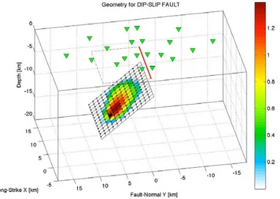
b) a rupture on a dipping fault with purely thrust-faulting motion.
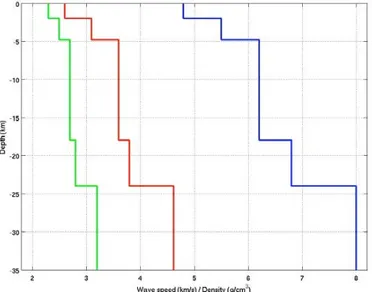
In both cases, we used the same layered isotropic velocity-density structure, simplified from the “generic” California rock-site velocity model (figure 2-5) of Boore and Joyner, (1997).
Validation
The quality factors QS and QP are assumed infinite
everywhere, because the Compsyn code does not account for the anelastic attenuation.
Figure 2-5: Velocity-density model for extended-fault forward-modeling
simulation.
Full-wavefield forward simulation of the velocity time-series has been performed from 0.05Hz up to 5.0Hz.
This validation test is based on exercises of the Source-Inversion Validation (SIV, web site: ttp://the siv.usc.edu/main/Home) a project, initiated and leaded by Martin Mai (KAUST).
2.4.1. Case: Strike-slip fault
In the first case-study, we generated the synthetic seismograms for a strike-slip source having the characteristics listed below:
Dip = 90°, Strike 90°, rake 180°;
Fault dimensions 13 km along-strike, 12 km down-dip; Discretization of rupture: node spacing is 0.5 km in each
fault-plane direction;
Seismic moment10F11: M0=1.658 ∙ 10 Nm (Moment
magnitude11F12Mw=6.11);
Hypocenter depth:14 km;
Rise time variable over the fault;
Rupture velocity variable over the fault;
An non uniform slip distribution of slip (as shown in figure 2-6).
11Seismic Moment:The seismic moment M0is defined as:
M0=μ∙average slip∙fault area
where is shear modulus 2.
12 Moment Magnitude:It is a magnitude scale, introduced by Hanks and
Kanamori (1979) based on the seismic moment of an earthquake (Mw):
Case: Strike-slip fault
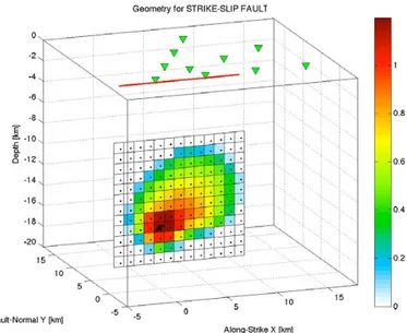
Figure 2-6: 3D-view of the rupture plane with an inhomogeneous slip
distribution, colored-coded according to the amount of the slip (in m). The black star denotes the hypocenter.
The receivers configuration consists of three linear arrays: one fault-parallel at the surface projection of the fault and two inclined arrays at 30° and 60° from the fault parallel array (figure 2-7).
Figure 2-7: Source-receiver geometry for a strike-slip fault case. The red
star shows the epicenter at X=0, Y=0 in a right-handed coordinates system with positive X pointing East, positive Y pointing North. The red line indicates the vertical projection of the updip-edge of an extend fault plane at depth.
On the ground of these parameters, we simulated the velocity seismograms with the STuDenT code and with Compsyn.
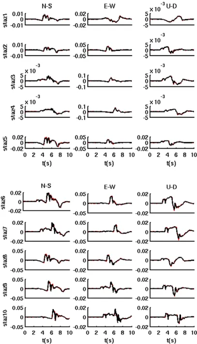
We show the three components of the time series in figure 2-8, and the spectral amplitudes in figure 2-9. The seismograms generated by STuDenT are in red, while the seismograms generated by Compsyn are in black.
Case: Strike-slip fault
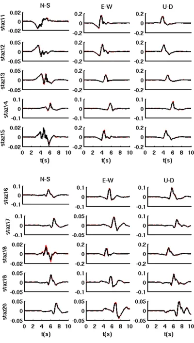
Figure 2-8: Comparison between STuDenT and Compsyn for all ten
station, and for the three component (N-S: North-South; E-W: East-West; U-D: Up-Down). The seismograms generated by STuDenT are in red, while the seismograms generated by Compsyn are in black. Each pair of theoretical seismograms is plotted with its amplitude scale (m/s).
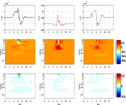
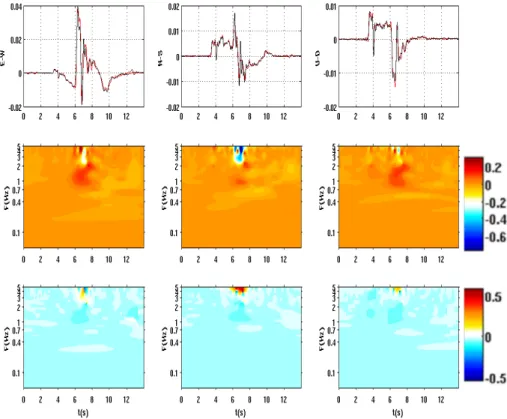
Figure 2-9: Comparison, in frequency domain, between STuDenT (red)
and Compsyn (black) for all ten stations, and for the three component (N-S: North-South; E-W: East-West; U-D: Up-Down).