Adaptive and quality driven approach to data management for wireless sensor networks

(1)

(2)

POLITECNICO DI MILANO V Facolt`a di Ingegneria

Corso di laurea in Ingegneria Informatica

ADAPTIVE AND QUALITY-DRIVEN APPROACH

TO DATA MANAGEMENT

FOR WIRELESS SENSOR NETWORKS

Relatore: Prof. Fabio A. SCHREIBER Correlatore: Ing. Cinzia CAPPIELLO

Tesi di Laurea di:

Federico ROSSINI Matr.740075 Matteo RUGGINENTI Matr.740504

(3)

Matteo: Alla mia famiglia, ai miei amici. Federico: Alla mia famiglia, ai miei amici, a Rachele.

(4)

Abstract

Wireless sensor networks (WSNs) are attracting great interest in a number of appli-cation domains concerned with monitoring and control of physical phenomena, as they enable dense and untethered deployments at low cost and with unprecedent flexibility. Nevertheless, due to the sensors size, their associated resources, in terms of memory and energy, are limited. Compression data algorithms address this issue by aggregating similar input values and sending to the base station the value generated by the compres-sion, reducing, in this way, the number of packet transmissions. MAC layer protocols, though, handle the activity period of the devices, affecting the direct proportion be-tween number of sent packets and energy consumption. For this reason, reducing the number of transmissions by itself, results to be insufficient for the energy saving goal. Furthermore, different monitored phenomena call for different network quality require-ments. The purpose of this work is, starting from an existing aggregation algorithm, to create a system that, at run-time, adapts a set of parameters, such as MAC layer and aggregation algorithm ones, in order to enhance a set of quality dimensions, according to the network quality requirements.

(5)

Acknowledgements

(6)

List of Figures

2.1 Taxonomy for a WSN application . . . 21

3.1 System architecture . . . 26

3.2 Windowing on data stream . . . 27

3.3 a) Expected trend, b) Slow Change, c) Fast Change and d) Irregular trend 30 3.4 Star and peer-to-peer topology examples . . . 39

3.5 Superframe structure without guaranteed time slots (GTSs) . . . 40

3.6 An example of the superframe structure . . . 41

4.1 An example of network configuration . . . 46

4.2 An example of the redundant information approach: changes in network configuration . . . 49

4.3 An example of the redundant information approach: base station data management . . . 50

4.4 An example of fault detection . . . 51

4.5 Example of state flow of the action-based approach. . . 60

4.6 Consumed Energy as FO and BO change. . . 63

(9)

4.8 Consumed Energy as the number of GTSs changes. a) Beacon Order =

6. b) Beacon Order = 8 . . . 65

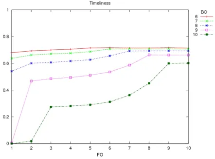
4.9 Timeliness as as FO and BO change. . . 66

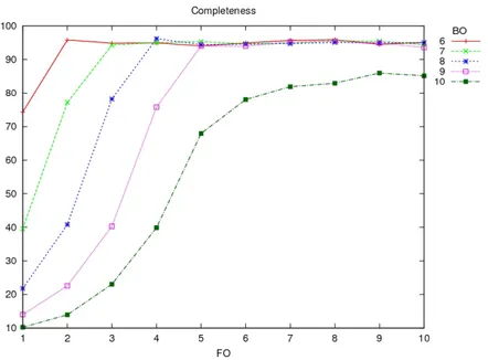
4.10 Completeness as FO and BO change. . . 68

4.11 Lost packets due to buffer overflow. . . 68

4.12 Lost packets due to interference. . . 69

4.13 Completeness in General and Packet Retrieval configurations with very high packet rate . . . 70

4.14 Completeness in General and Packet Retrieval configurations with lower packet rate . . . 71

4.15 Timeliness in General and Packet Retrieval configuration . . . 72

4.16 Completeness and different GTSs . . . 72

5.1 The modules and their connections in Castalia . . . 77

5.2 The node composite module . . . 78

5.3 Beginning of a configuration file . . . 79

5.4 Module parameters in the configuration file . . . 79

5.5 Application parameters in the configuration file . . . 79

5.6 Modules hierarchy . . . 80

5.7 Path loss parameters . . . 81

5.8 Typical temporal fading in wireless . . . 82

5.9 Network configuration during the simulations . . . 83

5.10 Input signal of each simulation . . . 85

5.11 Dimension values for different configuration as the completeness has the priority. (Samplinginterval = 10ms) . . . 86

5.12 Dimension values for different configuration as the completeness has the priority. (Samplinginterval = 100ms) . . . 87

5.13 Dimension values for different configuration as the energy has the priority. (Samplinginterval = 10ms) . . . 88

(10)

5.14 Dimension values for different configuration as the energy has the priority. (Samplinginterval = 100ms) . . . 88 5.15 Dimension values for different configuration as the timeliness has the

pri-ority. (Samplinginterval = 10ms) . . . 89 5.16 Dimension values for different configuration as the timeliness has the

pri-ority. (Samplinginterval = 100ms) . . . 90 5.17 Comparison among the three aggregation algorithms . . . 91 5.18 Dimension values for different configuration as the timeliness has the

pri-ority, using the LTC algorithm. (Samplinginterval = 10ms) . . . 92 5.19 Dimension values for different configuration as the energy saving has the

priority, using the LTC algorithm. (Samplinginterval = 10ms) . . . 93 5.20 Dimension values for different configuration as the energy saving has the

priority, using the Lazaridis et al. algorithm. (Samplinginterval = 100ms) 94 5.21 a) Original signal (green) and value received by the base station (blue);

b) Original signal (green) and interpolation of received data (blue) using Schoellhammer et al. algorithm . . . 95 5.22 a) Original signal (green) and value received by the base station (blue);

b) Original signal (green) and interpolation of received data (blue), using Lazaridis et al. algorithm . . . 96 5.23 a) Original signal (green) and value received by the base station; b)

(11)

List of Tables

3.1 Algorithm input and output . . . 33

3.2 Similarity Assessment . . . 33

4.1 Status each sensor can assume . . . 47

4.2 Adaptation actions . . . 56

4.3 Set of rules, grouped by quality metric . . . 73

5.1 Action-based approach parameters . . . 84

(12)

1

Introduction

Wireless sensor networks (WSNs) are attracting great interest in a number of ap-plication domains concerned the monitoring and control of physical phenomena, as they enable dense and untethered deployments at low cost and with unprecedented flexibil-ity.

WSNs are distributed systems typically composed of embedded devices, each equipped with a processing unit, a wireless communication interface, as well as sensing and/or ac-tuation equipment [1]. Sensors are equipped with capabilities to store information in memory, process information and communicate with neighbors and with a base sta-tion [2].

Such devices cooperatively monitor physical or environmental conditions (such as temperature, pressure or pollution level) of a certain habitat [3].

Initially introduced for military intents (such as military zone surveillance), nowa-days WSNs are used in public contexts such as habitat monitoring, health care, au-tomatic systems in houses and offices and traffic control. This has been eased by the rapid advancement of semiconductor manufacturing technology, which enabled electronic devices to get smaller, cheaper, and to require less power for their operation every year.

(13)

So far, many applications have been proposed that show the versatility of this technology, and some are already finding their way into the mainstream. Most often, in these scenarios tiny battery-powered devices are used for ease of deployment and in-creased flexibility [4]. This enables embedding processing and communication within the physical world, providing low-cost, fine-grained interaction with the environment.

However, due to the sensors size, their associated resources are limited. In such a context, the main cause of energy dissipation is the use of the wireless link. Solutions that minimize communication are needed [2]. Aggregation algorithms are approaches that aim to reduce sensors power consumption by aggregating information while they sense, processing the information and eventually sending the processed data [3].

Data compression is one effective method to use limited resources of WSNs. It is assumed that some loss of precision in the compressed version of incoming data can be tolerated if this helps in reducing communication. However, it is important that some data quality requirements are satisfied and the error introduced in the compression is below a specified threshold [2].

For this reason a set of quality metrics is also needed to classify the data and the sending node in order to take future decisions according to quality requirements. In this sense, the system must be quality-aware.

Furthermore, the assessment of the quality of a data source is context dependent, i.e. the notions of “good” or “poor” data cannot be separated from the context in which the data is produced or used [5]. For instance, the data about yearly sales of a product with seasonal variations might be considered quality data by a business analyst assessing the yearly revenue of a product. However, the same data may not be good enough for a warehouse manager who is trying to estimate the orders for next month.

This turns our needed solution into an adaptive system, i.e. a system that adjust its behavior according to the perception of the environment and the system itself. In this way, the system takes decisions accordingly to the context surrounding it.

(14)

Our work aims to address the formerly mentioned issues proposing a solution by means of a cross-layer aggregation data algorithm that allows to find a good trade-off among all the data quality metrics (in terms of timeliness, completeness and accuracy) exploiting information given by the context.

The algorithm, working in both the application and the communication layer, guar-antees that a satisfying output signal is received by the base station especially thanks to its reasoning capabilities. The base station, in fact, according to its knowledge and the current context is able to take decisions on the current state of the network, such as changing application or communication parameters or turning on/off certain nodes, in order to improve one or more specific dimensions of the data quality.

In Chapter 2 we describe the State of the Art, introducing the basic concepts of WSNs and theirs taxonomy, and compression data algorithms.Then, in Chapter 3, we focus on our aggregation data algorithm, describing its features and functionalities since it will be used on each sensor of the network to process data. Our quality-aware and adaptive approach is fully described in Chapter 4, where we list the quality metrics and the actions that drive the decisions taken by the base station accordingly to the context. In Chapter 5 we first introduce Castalia, the simulator used during the experimentation phase and we describe the environment of our experiments and simulations. Finally, in Chapter 6, we analyze the results of our experiments and we address possible future works.

(15)

2

State of the Art

In this chapter we describe the state of art of WSNs. We start by analyzing the sensors and WSNs underlying their limitations in terms of memory and energy consump-tion. Existing approaches that address these issues, such as compression data algorithms, are then presented and briefly described. We then describe how adopting specific access policies to the communication medium can affect the power consumption too. Data compression, though, leads necessarily to data quality loss, thus a trade-off between en-ergy saving and data quality requirements must be found. For this reason we introduce data quality metrics to assess the data quality according to the requirements. Finally, we present a taxonomy for WSNs to help to classify the different kind of applications and to ease the further analysis of our approach.

2.1 Introduction to Sensors and Wireless Sensor Networks

A Wireless Sensor Network (WSN) is a network where autonomous devices, spa-tially distributed, use sensors to cooperatively monitor the physical or environmen-tal conditions (such as temperature, pressure or pollution level) of a certain habi-tat [6].

(16)

as well as sensors and/or actuators. Sensors are equipped with capabilities to store information in memory, process information and communicate with neighbors and with a base station.

Initially introduced for military intents (such as military zone surveillance), nowa-days WSNs are used in public contexts such as habitat monitoring, health care, au-tomatic systems in houses and offices and traffic control. This has been eased by the rapid advancement of semiconductor manufacturing technology, which enabled electronic devices to get smaller, cheaper, requiring less power for their operation every year.

Smaller sizes lead to more limited resources available. In particular, the limitations that have the biggest impact during the design phase are the on-board memory size and the power consumption. Sensors can store only few pieces of data, possibly compressed, for a limited lapse of time. Thus, frequent transfers of data to a device equipped with a larger memory (base station) is needed. On the other hand, battery life-time is limited as well and data transmission is the function requiring the highest energy consumption effort. These two limitations are thus in conflict with each other. It is essential to find a good trade-off between the usage of memory and the amount of consumed energy in order to have a proper amount of free memory for data processing without, on the other hand, causing much power consumption.

Valid solutions to address this problem can be, as described in Section 2.2, data compression algorithms. Furthermore, changing the policies of accessing the communi-cation medium can also affect the power consumption, as shown in Section 2.3

2.2 Data Compression Algorithms

Data compression is one effective method to use the limited resources of a WSN [2]. Assuming that a, possibly small, loss of precision can be tolerated, we can send a com-pressed version of incoming data, in order to reduce the usage of the communication link. However, compression must be performed wisely, according to some data quality

(17)

requirements; in this way the error introduced during the compression phase can be below a specified treshold.

Traditionally, data compression approaches focused on saving storage without car-ing about energy consumption. As a result, the compression ratio is their fundamental metric. However, in the WSNs context, the focus must turn towards energy saving as well. In this way, new design issues arise and have to be addressed [7], calling for new approaches [8].

For this reason, most of the existing data compression algorithms are not suitable in the WSNs field given their size and complexity. However, in literature is possible to find interesting contribution to the data compression studies in the sensor networks context.

For example in [9] the authors address the analysis of high spatial correlation in data from fixed sensors in dense networks. Here, the context is specific and the addressed problems have particular characteristics and criticisms. As described in Chapter 3, the approach we adopted aims at handling data from different type of systems. In other words, we want our approach to be able to adapt and work correctly even in mutable scenarios.

Data compression has been mostly studied to enable in-network processing; with this term we describe those techniques that process data on a node or group of nodes before forwarding it to the user or to the base station. The goal of in-network process-ing of data streams is to select and give priority to reportprocess-ing the most relevant data gathered [10].

In this field, two different compression techniques are most widely used: spatial and temporal compression techniques.

Spatial compression deals with data redundancy in a same physical area. Significant contributions in this field propose models that, using specific functions, find similar values in order to aggregate and send them [11]. In [12], similar values compose the base

(18)

signal used to forecast and evaluate the collected data. In spatial compression analysis, the research contributions on sensors communication paradigms are extremely relevant (e.g., [13]).

Temporal compression is suitable for those contexts where the main goal is to detect data trend changes over time. Considering this scenario, one of the main contribution is a lightweight linear approach [14][15]. The use of linear compression provides a good balance between maximizing compression and minimizing processing complexity for each node. The approach considers the different measure points at different time instants. Each point is compared with the previous one and it is transmitted only if the measure is significantly different. In scenarios where phenomena are quite stable, this approach is very suitable. On the other hand, in case of unstable data, the algorithm would send the measured values one by one, wasting the energy of the sensor.

As we describe in Chapter 3, the data compression algorithm we deploy in each sensor of the network aims at detecting run-time data trend changes as the linear com-pression algorithms, but it is also able to maximize the comcom-pression even when the change in data trend is frequent. This feature makes it suitable for any situation regardless the phenomenon characterization.

Furthermore, the algorithm we adopted is also based on the concept of time series as [16][17][18]. In [16] the authors propose to perform on-line regression analysis over time series on data streams. Autoregressive models built on each sensor are instead used in [17] to forecast time series and approximate the value of sensors readings. Lazaridis and Mehrotra [18] also propose to fit models to time series, but they try to improve system performance, rather than doing regression analysis.

However, data compression is just the first step in the energy saving path, but it is not the only one. Furthermore, data compression leads necessarily to data quality loss. Our approach starts from a data compression algorithm, but adopts other policies and methods to reduce the energy consumption ensuring an acceptable level of data quality. In particular, while all the formerly mentioned approaches are basically sensor-oriented,

(19)

our proposed approach is network-oriented, since we think data quality depends on the capability of the sensor to provide data with an as little as possible error, as well as on the capability of the network itself to understand the context and to adapt to it. In this way, our algorithm is able to adopt to sudden data trend changes and to unexpected situations, such as faulty sensors, providing a higher level of quality and reliability of data.

2.3 MAC Layer Protocols

The boundaries between programming abstractions and the rest of the software executing on a WSN node is often blurred [1]. The limitations on WSN nodes, in terms of computing and communication resources, along with their application-specific nature, drive necessarily to a cross-layer design approach where not only the application layer is involved, but rather the design interweaves the application layer with other layers or system-level services.

An important element of this cross-layer design approach concerns the usage and exploitation of the Medium Access Control (MAC) layer. In fact, MAC protocols for WSNs strongly affect the access to the communication media and the energy consump-tion. Obviously, the goal in the adoption of a MAC protocol rather than another is to guarantee an efficient access to the communication link while carefully managing the en-ergy consumption of the nodes. The former goal is achieved adopting different policies, as latterly described; the latter is typically achieved by switching the communication link (the radio) into a low-power mode according to the transmission schedule.

Most of the existing MAC protocols fall in two categories. Contention-based proto-cols (e.g., [19][20][21]) regulate the access to the physical layer opportunistically, accord-ing to the current transmission requests. This class of protocols is surely easier to imple-ment and better tolerates nodes joining or leaving. Time-slotted protocols (e.g., [22]), instead, assign the nodes with predefined time-slots to schedule their transmissions over

(20)

time, providing a higher reliability and greater energy savings.

Typically, in other wireless platforms different from WSNs, MAC functionality is performed at a hardware level. In the WSNs context, instead, MAC protocol is imple-mented mostly in software, exploiting the low-level language associated with the operat-ing system. For this reason it is important to adopt a cross-layer design approach in order to optimize the overall performance of the algorithm, in terms of energy consumption and radio access.

In our work, we take into consideration this issue and adopt a highly widespread protocol known in literature as the IEEE 802.15.4 standard. Nevertheless, as described in Chapter 4, we made a few changes in the adopted standard in order to better satisfy our quality data needs and requirements giving our application a cross-layer conforma-tion.

2.4 Data quality

As mentioned in the previous section, data compression leads necessarily to data quality loss. Compression, thus, must be performed wisely, according to some data quality requirements.

The algorithm we adopted is able to deal with all types of trends and not only with a limited set as the algorithm proposed by [18]. This feature derives from an adaptive mechanism to change its parameters according to the data stream changes. This adaptation in data stream management is driven by data quality requirements. Several contributions in the literature adopt a similar approach by considering a different set of dimensions; for example, [23] monitors the processing delay to assure data freshness. The total response time is also checked in [24] to optimize the overall QoS performance according to the network condition and work load at run-time.

(21)

in this field, the most important component of cost is the energy consumed in providing the requested data. In [25] [26] [27], this cost versus quality metrics trade-off has been thoroughly analyzed.

The attitude among the authors of all these mentioned approaches is to discard out-liers and try to detect the value trend. In the algorithm we adopted, instead, outout-liers are important elements of the data stream to consider and store since scientific researchers deem they can be very useful in studying and interpreting natural phenomena.

In addition, we consider other data quality dimensions, such as accuracy and pre-cision, to improve the efficiency of the algorithm. However, these are metrics useful only for the sensor-side quality awareness. We, thus, added other metrics (e.g. complete-ness) and criteria to satisfy data quality requirements at a network level at run-time, as described in Chapter 4.

2.5 WSN Taxonomy

WSNs are being employed in a variety of scenarios. Such diversity translates into different requirements and, as a result, different programming constructs supporting them. In this section we identify some of the most common and important features of WSN applications that strongly affect the design of programming approaches, introduc-ing the taxonomy suggested in [1]. This description will help to better understand the configuration of our proposed algorithm. Figure 2.1 illustrates the dimensions considered by the authors.

Goal. In most WSN applications the goal is to gather environmental data for later, off-line analysis. A network of sensor-equipped nodes funnels their readings, possibly along multiple hops, to a single base station. Typically the base station is much more powerful (in terms of memory and energy) than a sensing node and acts as a data sink, collecting the network data. Along with sense-only scenarios, there is another class of applications where WSN nodes are equipped also with actuators;

(22)

Figure 2.1: Taxonomy for a WSN application

in this sense-and-react scenario, nodes can react to sensed data, closing the control loop [28].

Interaction pattern. Another key point in WSNs is how the nodes interact with each other within the network, which can be affected also by the application goal they are supposed to to accomplish. In particular, in a sense-only context a many-to-one interaction pattern is mostly adopted, where all sensors data is sent to a central collection point. However, one-to-many and many-to-many interactions can also be found. The former are important when it is necessary to send configuration commands (e.g., a change in the sampling frequency) to the nodes in the network; the latter is typical of scenarios where multiple data sinks are present, as it happens in a sens-and-react context.

Mobility. According to the need of the application, it is possible to deal with a certain degree of dynamism within the network. Mobility may manifest itself in different ways:

– In static applications, neither nodes nor sinks are able to move once deployed. This is by far the most common scenario in WSNs.

(23)

or animals. A typical case is wildlife monitoring where sensors are attached to animals, as in the ZembraNet project [29].

– Some applications, instead, exploit mobile sinks. The nodes may or may not move: the key aspect is that data collection is performed opportunistically when the sink moves in proximity of the sensors [30].

Space and time. The phenomena considered in the environment strongly affects either the different portions of the physical space, and the instants of time the distributed processing works. Regarding the space dimension we can classify the distributed processing in:

– Global, in applications where the processing concerns the entire network, typi-cally when the phenomena of interest span the entire geographical area where the WSN is deployed.

– Regional, in applications where the majority of the processing occurs only within some limited area of interest.

Concering the time dimension, instead, the distributed processing can be:

– Periodic, in applications that continuously sense and process data.

– Event-triggered, in applications mostly characterized by two phases: i) during the event detection, the system is mostly quite and the nodes monitor the phenomena with little or no communication involved; ii) in case the event condition is satisfied (e.g., a sensed value is above a certain threshold), the distributed processing is triggered.

Introducing the taxonomy helps to describe clearly the basic configuration, widely analyzed in Chapter 4, of our approach, according to the formerly listed dimensions.

In terms of goal, our application is sense-only. The base station takes decisions according to the values received and the context affecting only nodes and thus network behaviors. Actuators changing environment conditions are not involved. During the

(24)

sensing, the nodes periodically send their aggregated values to the base station. Thanks to its adaptiveness, the base station is also able to change at run-time a set of parameters (e.g., aggregation parameters) according to the received values or context condition and communicate them to the nodes of the network. In this sense, our approach exploit a combination of many-to-one and one-to-many interaction patterns. In our algorithm the base station triggers actions according to a set of rules based on events (e.g., a cer-tain data quality metric is not satisfied anymore), giving it an apparent event-triggered configuration. Nevertheless, since the conditions are checked at the base station by periodically collecting data, such application falls in the periodic class and not in the event-triggered one. Furthermore, our field of interest is divided into different zones and the base station reasoning is focused differently on each zone. In this sense, in our approach the distributed processing works with regional logic. Finally, none of the nodes of the network are able to move. In terms of mobility, thus, our network is static.

(25)

3

Technologic State of the Art

In our former work (i.e. [3]) we implemented and tested an aggregation data algorithm on a Mica2 mote. The experimentation, though, was limited to a sensing and a processing phase performed by just one sensor, sending periodically aggregated values to the base station.

This simplistic network configuration was due to its particular goal. Our purpose then, in fact, merely concerned the analysis of the efficiency of the proposed approaches, in terms of data quality and energy savings on the single node.

Even though its simplicity helped to fully analyze the algorithm behaviors in dif-ferent case studies, it does not represent a realistic network scenario. For this reason, the intent of the present work is to expand the approach of [3] to a more realistic net-work scenario, adding several nodes to the netnet-work, all equipped with our aggregation data algorithm. This led us to adopt a MAC layer protocol to improve communications between nodes, and to add also new functionalities to ensure network stability and a high data quality level as described in Chapter 4.

In this chapter we first introduce the reader to the basic features of our starting aggregation data algorithm. We, then, describe the basic features of the MAC layer protocol we adopted, namely IEEE 802.15.4 standard.

(26)

3.1 System Quality Requirements

In a wireless sensor network, a set of queries Q is submitted to the base station to get the desired data. The base station then, forwards the queries to the WSN in order to gather sensors data. The quality of the data provided by a sensing application is a combination of different quality metrics. Quality requirements are typically used by the base station to collect only the most relevant data.

In our aggregation data algorithm, the behavior of each sensor is influenced by the following requirements: each sensor node just collects and sends data in order to satisfy all the quality requests [31]. Quality requirements specify constraints in terms of accuracy and precision. The former is the main variable that identifies the measurement quality and enable the system to detect possible errors or changes in the input data stream trend. Typically, it is defined as the degree of conformity between a measured or processed quantity with its corresponding actual value [2]. Since in a sensing scenario it is impossible to know a priori the real value, our algorithm compares the sensed value with a value of reference to calculate its accuracy. This value is set at design time and represents the expected value to be measured. Obviously, the phenomena of interest may change in time; for this reason, the algorithm changes the value of reference at run-time in order to adapt to the context under exam. Accuracy is thus measured using the sensed value and this value of reference as follows:

Accuracy = abs(sensedV alue − vRef )

The algorithm takes decisions according to the value of accuracy. A value is con-sidered accurate if it respects a accuracy threshold called aTolerance as shown in Pro-gram 3.1.

The latter is the degree to which further measurement show the same or similar results [32]. How these quality dimensions impact on the data stream management is

(27)

Program 3.1 Accuracy assessment int checkAccuracy(double val) {

if(fabs(sensedValue - Vref) < aTolerance) return 1;

else

return 0; }

discussed in the next sections of this chapter.

3.2 System Architecture and Data Structure

The input data stream can be seen as a continuous flow of real-time data tuples of the form < sensor-id, timestamp, value > coming to the sensor’s input buffer. As in many real-time systems, we can imagine the Input Buffer (IB) split into two different storage areas (i.e., IB1 and IB2). Initially, data are stored into IB1 until it is full, then

input data are fed to IB2. Meanwhile data in the first buffer are transferred to the

compression engine to be sent to the output buffer as shown in Figure 3.1. Analogously, when the compression is performed, data stored in IB2are transferred to the compression

engine, and incoming data are fed to IB1.

Figure 3.1: System architecture

(28)

infinite data stream is reduced to a sequence of finite time-ordered data sets on each of which the compression algorithm can work [2]. Furthermore, the main window can be partitioned itself into smaller sub-windows (see Figure 3.2) ; values in this kind of sub-windows are considered so similar that can be aggregated by computing their average.

Figure 3.2: Windowing on data stream

The algorithm reduces the communications by sending the base station only the average values and the outliers, i.e., those values that depart from the expected trend and could stand for either a measurement error or a sudden change in the measured phenomena. . The former are sent together with the timestamps of the first and the last value which took part to the aggregation; the latter are associated with the actual timestamp in which they are sensed by the node. Dealing with the timestamps is a fundamental aspect of this approach since it allows to re-build the incoming signal once the base station received the aggregated data.

The sub-windows shown in Figure 3.2 may change in terms of size according to the similarity of the values involved in the data stream. The similarity concept is defined by considering the two formerly mentioned data quality dimensions of accuracy and precision. Accuracy can be identified with the window’s height; in particular, the window height influences the accuracy of the measure and the robustness in finding outlier values. To understand whether the value falls into one case or the other we need to measure its precision. Indeed, if the values are not accurate (outside the window height), but precise, it means that they are not similar to the reference value, but they are characterized by a small standard deviation. This means that a change in the system

(29)

under control has occurred.

Another possible scenario occurs when data values are not accurate nor precise; this happens when the trend in the measured phenomena is very irregular. On the other hand, a measurement error is an occasional and isolated event and all the other values are still considered accurate and precise. The different cases are all formally described in Section 3.3 .

As the sub-window height do, also the sub-window width plays an important role in this approach. It, indeed, affects the compression amount: the larger the number of points in the window, the larger the compression we get. On the other hand, a window with a single point corresponds to no compression whatsoever. It is important to underly, though, that in case the sampling interval is very low (high data rate), enlarging the sub-window width can decrease the overall network traffic. In fact, if the phenomena under exam is stable enough, the larger the window, the the more aggregation and thus the less packet sent. As illustrated in Chapter 4 this factor results to be very important to control the network traffic and preserve the network quality requirements.

3.3 The Model

In this section, we focus the description on the interaction between a single data producer (sensor) and a data archiver (database located in the base station). Our aim is to describe the sensor’s behavior rather than the data processing and reasoning per-formed by the base station, which are, instead, described in Chapter 4.

3.3.1 Preliminaries

Each sensor has a sampling frequency that affects the time instant ti in which data

are acquired. Considering these time instants, we define a value series

(30)

as a set of values observed in subsequent n time instants. The maximum number of measure points N represents the cardinality of data in the input buffer (window width). Sub-windows are characterized by their width W and height H. The former coincides with the number of points in a sub-window and affects the compression factor accord-ing to the data trend variability. The latter represents the biggest difference between two measure points in the same window and sets the accuracy tolerance affecting the robustness in finding outlier values.

The quality-oriented approximation starts from the definition of the requirements about accuracy and precision, which can be set by the user. In continuous value moni-toring, accuracy and precision can be used to detect errors or changes in the monitored phenomena. Precision is typically assessed by mean of the standard deviation of the measured values. The smaller the standard deviation, the higher the precision. On the other hand, accuracy can be defined as the error expressed by the difference between the measured value and a reference value (i.e., vref in Figure 3.2).

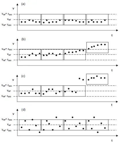
As mentioned in Section 3.2, different combination of accuracy and precision dis-tinguish different scenarios in the input data trend, as shown in Figure 3.3:

1. Expected trend : values are either precise and accurate; as a consequence the trend is regular;

2. Slow Change: the trend is characterized by an unexpected, but not permanent and small variation. Values are still precise but not accurate anymore;

3. Fast Change: similar to the former; in this case,though, the trend is charac-terized by an unexpected, but lasting and large variation in a way that precision requirements are satisfied again sometimes after the instant at which the variation occurred;

4. Irregular/Bursty trend : the trend is characterized by unexpected and discon-tinuous variations. Values are not precise but they can be both accurate or inac-curate.

(31)

Note that any data stream can be represented as the combination of the described trends with possible outlier values. Outliers are identified in all cases in which both accu-racy and precision requirements are not satisfied, but the overall trend has not changed (in Figure 3.2, the dot inside the circle). Outliers might hide significant information and should not be discarded. In fact, analyzing historical series, outliers sometimes reveal periodical, and thus systematic, irregularities that can not be inferred with a local and limited analysis.

Figure 3.3: a) Expected trend, b) Slow Change, c) Fast Change and d) Irregular trend

The sensor has a finite energy supply which is consumed during normal sensing operation at some rate. Additional energy drains are caused when using any of the sensor equipment, namely (i) powering its memory, (ii) using its CPU, (iii) sending/receiving

(32)

data. The rates of energy consumption for these operations are sensor-specific. Typically, communication is the major cause of energy drain in sensors and hence, since our interest is to extend sensor’s life, communication must be limited. For this reason, each sensor is characterized by:

et : energy consumption for the transmission of one byte;

ee : energy consumption for processing one instruction;

Et : energy consumption for data transmission to the base station;

Ee : energy consumption for processing analysis and aggregation algorithms;

Etot : total energy consumption of the sensor, calculated as Et + Ee.

Our approach aims at minimizing the total energy consumption assuming that et ee. In fact, the algorithm processes the input data stream in order to transmit to

the base station only the aggregated values and the possible outliers. Assuming Z to be the set of aggregated values, J the set of the outlier values and N the total number of values in the input data stream; the algorithm is considered efficient if the output is composed by (Z+J) values instead of N where (Z+J) N.

3.3.2 The Algorithm

In this section we detailedly describe our approach, showing its feasibility and adaptivity.

Setting the input parameters

The main input to be fed to the algorithm concerns the quality requirements. In our approach, as stated in Section 3.2, quality requirements are represented by the value accuracy and precision. Formally, we define accuracy as the difference between the measured value vnand the reference value vref, which represents the bias [32]. Assuming

(33)

εacc to be the tolerable error in a measured value, the measure is considered accurate

if:

|vn− vref| < εacc

Note that defining εacc corresponds to defining the height H of the sub-window since

H = 2 · εacc.

On the other hand, precision can be defined as the reciprocal of variance. In this way, a measure is considered precise if:

1/N ·

N X

n=1

(vn− µ)2 < εprec

where µ is the average calculated among all the vn values.

Other parameters needing to be set are the maximum number of points to consider in a sub-window W and the minimum number of outliers contained in a window L. The latter defines the threshold number of outliers in a single window after which the trend is considered to be irregular. In this case, the algorithm halts the aggregation function and sends the values one by one. Finally, it is necessary to specify the number of observation C needed to evaluate if the irregularities in a trend are only isolated events or are part of a permanent change in the trend.

Algorithm body

The input parameters and the outputs of the algorithm are listed in Table 3.1.

As mentioned in Section 3.2, the algorithm is based on the evaluation of the simi-larity of the incoming data with the previous data values acquired in the sensing activity. Similarity degree depends on the precision and accuracy assessment as described in Ta-ble 3.2.

The similarity assessment enables the algorithm to classify the current trend char-acterizing the input data and, thus, take the corresponding sequence of actions.

(34)

Name Symbol INPUT Time Series V=< v1, v2, . . . , vn>

Expected Value vref

Accuracy Tolerance εacc

Precision Tolerance εprec

Window Width W Continuity Interval C Minimum Outlier Number L

OUTPUT Aggregate values T=< t1, t2, . . . , tz >

Outliers O=< o1, o2, . . . , oj > Table 3.1: Algorithm input and output

The aggregation algorithm can be divide into three main phases:

1. Check possible values from previous windows;

2. Processing all the data in the buffer one by one;

3. Post-processing checks.

The first phase allows the system to correctly handle possible trend changes occur-ring among two different windows. The second phase can be considered the actual core of the algorithm. It, indeed, identifies and classifies the values in the current window according to their similarity value.

Accuracy Precision Similarity Trend Accurate Precise High Expected Trend Not Accurate Precise Medium Slow Change

Accurate Not Precise Low Irregular Trend Not Accurate Not Precise None Irregular Trend

Table 3.2: Similarity Assessment

We now illustrates the main algorithm steps in pseudo-code:

(1) Indata[w] = vw

Check accuracy and precision and evaluate the different cases. The algorithm anal-yses the different data streams trends described in Figure 3.3.

(35)

(2) SWITCH(εacc, εprec)

CASE 1: Data follow the expected trend. If we have analysed all the measure points in the buffer, the average of the acceptable values is calculated. The acceptable values are defined as all the stored values except for outliers. If the number of outliers is more than the threshold L then all the values will be transmitted without any further analysis.

(3) CASE (< εacc, < εprec)

(4) IF number of analysed values=W AND Number of outliers < L THEN t[z]=AVG(Acceptable values); Increment z

(5) ELSE IF Number of outliers > L

(6) THEN T= ht1, t2, ...tzi= V= hv1, v2, ...vwi

(7) ELSE Analyse new value and GO TO (1)

CASE 2: Data undergo a slow change. In this case when the algorithm detects an outlier, it controls if it is associated with a permanent or transient data trend change. In the former case, it calculates the average of the values stored before the exception and recalculates the expected value vref along the last inaccurate values. In the latter

case, inaccurate values are transmitted to the base station as outliers.

(8) CASE (> εacc, < εprec)

(9) Variable initializations: the number of unexpected values, the time instant in which the exception occurs (Te)

(10) O[j]=vw

(11) Indata[w]= vw+1

(36)

(13) INCREMENT the number of unexpected value and the number of outliers (14) O[j]=vw

(15) IF number of analysed values=W AND number of subsequent unexpected values = C (16) THEN t[z]=AVG(Acceptable values arrived before Te); Increment z ;

(17) t[z]=AVG(Acceptable values arrived after Te); Increment z;

(18) vref=AVG(Acceptable values arrived after Te)

(19) ELSE IF number of analysed values=W AND number of subsequent unexpected values<C (20) THEN t[z]=AVG(Acceptable values); Increment z;

(21) ELSE IF number of subsequent unexpected values = C

(22) THEN t[z]=AVG(Acceptable values arrived before Te); Increment z;

(23) vref=AVG(Acceptable values arrived after Te)

(24) Delete outliers from O[j] to O[j-C]

(25) GO TO 1

(26) else Indata[w]=vw+1and GO TO 1

CASE 3: Data are characterized by an oscillatory trend or bursts. The analysed value is classified as an outlier.

(27) CASE (< εacc, > εprec) OR (> εacc, > εprec)

(28) O[j]=vw

(28) IF number of analysed values=N AND Number of outliers < L THEN t[z]=AVG(Acceptable values); Increment z;

(29) ELSE IF Number of outliers > L

(30) THEN T= ht1, t2, ...tzi= V= hv1, v2, ...vwi

(37)

Energy Consumption

Given the nomenclature described in Section 3.3.1, the proposed algorithm can be considered efficient if

et· N > Ec+ et· Z + et· J

Note that, if the trend is particularly irregular, most of the values will be classified as outliers; therefore, if the number of outliers exceeds the threshold L, the algorithm is bypassed and all the values are transmitted one by one, saving, in this way, the additional computation energy consumption due to the aggregation process.

Cost-quality trade-offs

The outputs of the algorithm, in terms of aggregated data transmitted to the base station, and its relative energy consumption are mainly affected by the input parameter settings.

Changing in the precision, accuracy or continuity interval values strongly influences the output quality. In particular, high precision and accuracy requirements lead to higher number of values transmitted to the base station. Therefore, the higher the quality level required the higher the energy consumed. For this reason, quality requirements have to be properly designed according to the analyzed context. For instance, stable and not critical phenomena do not need high quality level, increasing energy saving benefits. On the other hand, irregular and critical contexts require high quality results since even the smallest system change should be detected and transmitted.

For this reason, the choice of the parameters values must be made wisely, on the basis of a previous knowledge of the application and its environmental deployment.

(38)

3.4 IEEE 802.15.4 MAC Protocol: a General Description

Providing quality of service (QoS) support is a challenging issue due to highly resource constrained nature of sensor nodes, unreliable wireless links and harsh operation environments.

Our previous work [3] intent concerned merely the analysis of the efficiency of the proposed approach, in terms of data quality and energy savings, only on a single node. In the present work, instead, we treat a more realistic scenario, focusing our attention at the whole network level. For this reason, it is necessary the adoption of different strategies and policies. In particular, we now focus on the QoS support at the MAC layer which forms the basis of the communication stack and has the ability to tune key QoS-specific parameters, such as the duty cycle of sensor devices.

MAC layer possesses a particular importance among them since it rules the sharing of the medium and all other upper layer protocols are bound to that. QoS support in the network or transport layers cannot be provided without the assumption of a MAC protocol which solves the problems of medium sharing and supports reliable communi-cation [33].

The MAC layer protocol adopted by our approach is the one defined by the IEEE 802.15.4 standard. The standard, which is used as a basis for the ZigBee, WirelessHART, and MiWi specifications, has been originally designed for low-data-rate WPANs. IEEE Std 802.15.4-2003, indeed, defined the protocol and compatible interconnection for data communication devices using low-data-rate, low-power, and low-complexity short-range radio frequency (RF) transmissions in a wireless personal area network (WPAN) [34].

As stated in Section 2.3, our algorithm adopts a cross-layer approach, dealing with both the application and MAC layer. For this reason, we now illustrate the main features of the standard, in order to provide the reader with some basic knowledge necessary to understand how the MAC layer behaves. In Section 4.3, instead, we show how changes in the protocol parameters can affect the overall data quality, in terms of the formerly

(39)

described metrics.

3.4.1 Introduction

An LR-WPAN is a simple, low-cost communication network that allows wireless connectivity in applications with limited power and relaxed throughput requirements. The main objectives of an LR-WPA are ease of installation, reliable data transfer, short-range operation, extremely low cost, and a reasonable battery life, while maintaining a simple and flexible protocol.

Some of the characteristics of an LR-WPAN are as follows:

– Over-the-air data rates of 250 kb/s, 100kb/s, 40 kb/s, and 20 kb/s

– Star or peer-to-peer operation

– Allocated 16-bit short or 64-bit extended addresses

– Optional allocation of guaranteed time slots (GTSs)

– Carrier sense multiple access with collision avoidance (CSMA-CA) channel access

– Fully acknowledged protocol for transfer reliability

– Low power consumption

3.4.2 Network Topologies

Depending on the application requirements, an IEEE 802.15.4 LR-WPAN may operate in either of two topologies: the star topology or the peer-to-peer topology (see Figure 3.4). In the star topology (he one adopted by our approach), the communication is established between devices and a single central controller, called the PAN coordinator. A PAN coordinator may also run a specific application, but it can be used to initiate, terminate, or route communication around the network. The peer-to-peer topology also has a PAN coordinator; however, it differs from the star topology in that any device

(40)

may communicate with any other device as long as they are in range of one another. Peer-to-peer topology allows more complex network conformations to be implemented, such as mesh networking topology.

Figure 3.4: Star and peer-to-peer topology examples

3.4.3 Functional Overview

A brief overview of the general functions enabled by the usage of the standard is given in the next sections to make the reader confident with the different parameters we take into consideration in Section 4.3.

Superframe structure

This standard allows the optional use of a superframe structure. The format of the superframe is defined by the coordinator. The superframe is bounded by network beacons sent by the coordinator (see Figure 3.5a) and is divided into 16 equally sized slots. Optionally, the superframe can have an active and an inactive portion (see Fig-ure 3.5b). During the inactive portion, the coordinator may enter a low-power mode. The beacon frame is transmitted in the first slot of each superframe. The beacons are used to synchronize the attached devices, to identify the PAN, and to describe the structure of the superframes. Any device wishing to communicate during the contention access period (CAP) between two beacons competes with other devices using a slotted CSMA-CA mechanism. All transactions are completed by the time of the next network

(41)

beacon.

Figure 3.5: Superframe structure without guaranteed time slots (GTSs)

Specifically, the structure of this superframe is described by the values of macBea-conOrder and macSuperframeOrder. The MAC attribute macBeamacBea-conOrder, describes the interval at which the coordinator shall transmit its beacon frames. The value of macBeaconOrder, BO, and the beacon interval, BI, are related as follows: for 0 ≤ BO ≤ 14, BI = aBaseSuperf rameDuration · 2BO symbols.

The MAC attribute macSuperframeOrder describes the length of the active portion of the superframe, which includes the beacon frame. The value of macSuperframeOrder, SO (in our work also referred to as F O), and the superframe duration, SD, are re-lated as follows: for 0 ≤ SO ≤ BO ≤ 14, SD = aBaseSuperf rameDuration · 2SO symbols.

The active portion of each superframe shall be divided into aNumSuperframeSlots equally spaced slots of duration 2SO·aBaseSlotDuration and is composed of three parts: a beacon, a CAP and a contention-free period (CFP). The beacon shall be transmitted, without the use of CSMA, at the start of slot 0, and the CAP shall commence immedi-ately following the beacon. The start of slot 0 is defined as the point at which the first symbol of the beacon is transmitted. The CFP, if present, follows immediately after the

(42)

CAP and extends to the end of the active portion of the superframe. Any allocated guaranteed time slot (GTS) shall be located within the CFP.

Figure 3.6: An example of the superframe structure

Figure 3.6 shows an example of a superframe structure. In this case, the beacon interval, BI, is twice as long as the active superframe duration, SD, and the CFP contains two GTSs.

Furthermore, we made a change in the MAC protocol behavior: when GTSs are used, if the MAC layer output buffer is filled for less than half of its size, the contention access period (CAP) will be disabled. In this way, the active period is formed by the only contention-free period (CFP); in other words, the sensor results to be active only during its time slot instead of the entire active period, resulting in a remarkable energy saving (see Section 4.3.2).

Power consumption considerations

As previously mentioned in Section 2.3, MAC protocols, affecting the access to the communication media have considerable effects on the energy consumption of each sensor.

In our previous work ([3]), we could assume that the power consumption, mostly caused by the transmission phase, was directly proportional to the amount of data

(43)

transmitted. This happened because in our first approach we did not adopt any kind of MAC layer protocol, turning on and off the radio whenever a piece of data was ready to be sent.

With the current approach, instead, the active period of the radio is dictated by the parameters of the MAC layer. In this way, the energy consumption is mainly affected by the duration of the active period rather than the number of sent packets (as shown in Figure 4.7 in Section 4.3.2).

The present work results to be a cross-layer application because, given the effects of the MAC layer on the energy consumption (and on the other data quality metrics, as shown in Section 4.3), we make the base station able to change MAC layer parameters at run-time in order to adapt to the context.

(44)

4

Methodology: Quality- and Context-aware algorithm

In this chapter we describe in detail the functionalities of our approach. We start by listing our data quality requirements defining quality metrics for the output. Fur-thermore, we illustrate some additional functionalities the network can adopt to enhance the data quality and the overall network reliability. Finally we analyze the adaptiveness of our approach. For this purpose, we present a study that enables us to understand how changing MAC and algorithm parameters affects the overall data quality in terms of quality metrics. From the results of this study, we introduce the actions the base stations adopt at run-time to autonomously adapt to the context.

4.1 Network Quality Requirements

As formerly stated, the main aim of our algorithm is to reduce the energy consump-tion preserving, at the same time, outgoing data quality in terms of pre-established qual-ity metrics. Since our approach is adaptive, it is fundamental to control these metrics at run-time, in order to take decisions in case values do not conform certain threshold.

Quality is assessed in terms of accuracy and precision dimensions in the aggregation data algorithm. Nevertheless, in this work we aim to provides a high quality data level to the entire network. For this reason, we refer to the following quality metrics: timeliness,

(45)

completeness and energy consumption. It is necessary, thus, to find a good trade-off among these dimensions according to the power consumption they imply.

Timeliness is the property of information to arrive early or at the right time. Typically it measured as a function of two elementary variables: currency and volatility [2]:

T imeliness = max(1 − Currency/V olatility; 0)s

where the exponent s is a parameter necessary to control the sensitivity of timeli-ness to the currency-volatility ratio. In our context, currency can be defined as the interval from the time the value was sampled to the time instant at which the base station receives the data. On the other hand, volatility is a static information that indicates the amount of time units (e.g., seconds) during which data is considered valid. Volatility is usually associated with the type of phenomena that the system has to monitor and depends on the change frequency. Timeliness constraints are one of the main drivers for data processing and transmission.

Completeness represents the amount of packets received in a defined window over a predefined window size (expressed in number of packets) [35].

Completeness(s(t)) = sW(t) W

where sW(t) is the amount of data received in the window W at time t, and W the

window size, in terms of packets. In this sense, the completeness of the a window is 1 if no packet is lost and is 0 if all the packets of the window are lost.

Energy consumption is a fundamental dimension in the network quality assessment. Theoretically, the base station cannot know the amount of energy consumed by each sensor at run-time, unless it is not explicitly communicated by the sensor. For the sake of simplicity, we made the base station able to know the energy level of each sensor without communicating it, exploiting the functionalities of the

(46)

sim-ulator we adopted (widely described in Section 5). In this way, the base station is aware of the overall power consumption and can take decision accordingly.

The adaption of different strategies can enhance one dimension or another. The choice of a MAC protocol rather than another, for instance, is a strategy itself and strongly affects all the former quality dimensions. In particular, in Section 3.4 we in-troduce the MAC protocol we adopted for our approach and in Section 4.3 we illustrate how changes in its parameters affect each dimension.

Besides the adoption of a MAC protocol, other functionalities can also affect the quality of the network in terms of quality metrics and reliability; these functionalities, such as data acknowledgment and faulty sensor detection, are fully described in Sec-tion 4.2.

4.2 Network Data Quality and Reliability

WSNs are being employed in a variety of contexts. Typically, such diversity trans-lates into different requirements and, in turn, different programming constructs sup-porting them. The intent of our work is to give an approach able either to adapt to the current context and to offer functionalities that the user can select at design time accord-ing to the system requirements. These latter functionalities can also be introduced at run-time in case the base station reckons one of them is needed to improve the network reliability or quality, in terms of quality metrics.

4.2.1 Fault Detection: Redundant information

Data quality dimensions are not enough to assess the overall quality of a network by themselves. For instance, let us assume a field divided into different zones. If monitoring the temperature of a zone the values of a certain sensor start plausibly drift to a different

(47)

value of reference the base station would still consider them as good values. In this case, though, if the drift was driven by some kind of event affecting only that sensor, the information about that zone would be corrupted and thus wrong.

Thus, the objective of the context system is to classify each sensor to the corre-sponding level of reliability, comparing, when needed, their values to values produced by other sensors in the same zone.

The Model

Assuming the monitored field divided into i zones, we can see each zone as a set of sensors Zi =< si,1, si,2, . . . , si,n>, where n is the total number of sensors deployed in

zone i. Figure 4.1 illustrates an example with a field divided into 4 zones with 3 sensors in each zone. During the start up, the base station chooses a leader for each zone (green sensor in the figure); the zone leaders are the sensors entitled to sense, aggregate and send data to the base station.

Figure 4.1: An example of network configuration

(48)

same zone (blue sensor in the figure). When the other sensors detect a change in the trend, a redundant information approach is used: the two sensors start sending their own values to the base station to compare their values to the leader’s ones for a previously established elapse of time in order to make the base station able to take a decision. The base station takes decision also according to the current status of the sensors. We defined different possible status as shown in Table 4.1

STATUS Meaning

LEADER The node is sensing and is the leader of the zone.

ON The node is entitled to sense and send data to the base station to control the leader’s values.

OFF The node is not sensing nor sending data to the base station.

UNRELIABLE The node has been labeled as unreliable, its values may be wrong.

FAULTY The node is broken and must be repaired or substituted.

Table 4.1: Status each sensor can assume

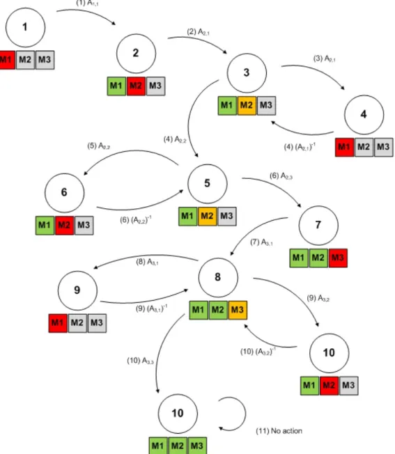
We now illustrates the main steps in pseudo-code:

a non-leader sensor (status ON) receives a value from leader sensor j in zone i. (1) sensorBuffer[k] = vsi,j

The sensor then compares the leader’s value to its own.

(2) IF abs(sensorBuffer[k] − sensedValue)< Control Tolerance)

(3) THEN GO TO (1)

(4) ELSE

(5) send(sensedValue, BaseStation)

(49)

On the other hand, when the base station receives a packet from a

the base station receives a value from sensor j (with status ON) and one from sensor k (status LEADER) in zone i.

The base station compare the sensor values to the zone leader ones.

(1) baseStationBuffer[k,i] = vsi,k

(2) baseStationBuffer[j,i] = vsi,j

(3) IF abs (baseStationBuffer[k,i] − baseStationBuffer[j,i])< Control Tolerance)

(4) THEN GO TO (3)

(5) ELSE

(6) start comparison()

At this point the algorithm checks the similarity among sensors values two by two increasing a counter each time the sensors values are similar.

(7) IF sensor leader has maximum similarity

(8) THEN GO TO (1)

(9) ELSE IF sensors ON have maximum similarity

The base station has to change the status of si,j into UNRELIABLE and promote

to leader one of the two sensors ON.

(10) status(Zi,j, UNRELIABLE)

(11) status(Zi,k, LEADER)

Obviously, this approach needs a configuration with at least three sensors per zone.

(50)

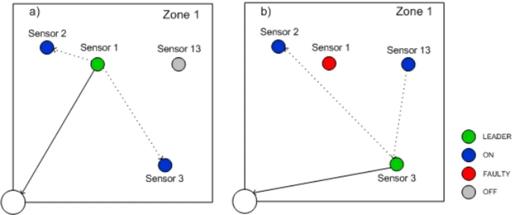
An Example

Let us consider a single zone with four sensors: Sensor 1, Sensor 2, Sensor 3 and Sensor 13. During the start-up phase, the base station randomly sets Sensor 1 as zone leader. Figure 4.2a shows zone 1 configuration. Sensor 1 is the leader (green), Sen-sor 2 and SenSen-sor 3 are simply ON (blue) while SenSen-sor 13 is OFF (grey). As shown in Figure 4.3, the zone leader starts sensing plausible values, according to the application parameters. At a specified time the simulator forces the data trend to drift from the expected value.

Figure 4.2: An example of the redundant information approach: changes in network configura-tion

When the ON sensors detects the drift, they start sending to the base station their values (see Figure 4.2b) to start the comparison. The comparison takes into consideration a number of samples set at design time; after this phase the base station notices that

(51)

Sensor 1 drift was not justified by the context and decides to promote Sensor 3 as the new zone leader, and sets Sensor 1 status as UNRELIABLE (Figure 4.2c) and set Sensor 13 status as ON for further comparisons.

In this way, we use a context information to categorize and increase the quality of measured data in our WSN. The context-aware controller, thus, is able to both increase the performances of the network classifying faulted data, enhancing the reliability of the sensor fusion.

Figure 4.3: An example of the redundant information approach: base station data management

Figure 4.3 shows also how the base station, thanks to the information retrieved during the monitoring, is able to reconstruct the trend of the data, in the example as-sumed to be a day-long temperature monitoring, by means of only the values considered as reliable.

As just described, this function is called when the values of the leader are drifting, but they are still plausible. On the other hand, if the base station detects an irregular

(52)

drift, for instance, measuring the environment temperature, a sensor reports 70oC (see Figure 4.4a) , without waiting for other ON sensors values for the comparison, it sets the leader zone as FAULTY, promotes one ON sensor to LEADER and sets one OFF sensor to ON (see Figure 4.4b).

Figure 4.4: An example of fault detection

4.2.2 Packet Retrieval

Considering a realistic scenario we cannot fail in taking into consideration also a possible packets loss. Indeed, in real networks several factors can affect the loss of packets. The wireless channel, described in Chapter 5, is one of the main factors affecting the correct transmission between nodes.

On the other hand a realistic design has to consider also other possible causes of packets loss such as output buffer overflow, collisions and interference.

Buffer overflow occurs when the output buffer is fed with data at a rate higher than the sending (and thus, emptying) rate. In this case, the system will discard the extra packets, causing a packets loss.

Collisions occur when two or more sensors try to access to the communication link at the same time. In this case the transmissions fail and have to be re-scheduled.

(53)

electro-magnetic induction or electroelectro-magnetic radiation emitted from an external source. The disturbance may interrupt, obstruct, or otherwise degrade or limit the ef-fective performance of the transmission. These effects can range from a simple degradation of data to a total loss of data.

Adopting a MAC layer protocol is a first step in trying to address these issues. In fact, increasing the active period (see Section 3.4.3), for instance, allows the sensor to send more data, lowering the possibility of buffer overflows to occur. Furthermore, most of the MAC layer protocols, including the one adopted in our approach, provide the system with a set of functionalities that help to detect or avoid collisions. In particular, the IEEE 802.15.4 protocol uses a slotted carrier sense multiple access with collision avoidance (CSMA-CA) mechanism [34]. In Section 4.3 we illustrate in detail how changes in MAC layer protocol parameters can affect the performance of the network underlying their effects on the quality metrics under exam.

Nevertheless, the MAC layer protocol could be not sufficient; in fact, the protocol can help in increasing the overall network performance, but in case the recipient (i.e., the base station) does not receive a packet the MAC layer cannot trace the loss. In fact, the main MAC layer concern is to correctly access the communication medium and not to guarantee the effective reception at the base station.

In this sense, each time a packet is not received the application is not notified and cannot detect the packet loss. For this reason, we introduced a packet retrieval functionality at the application layer to overcome this issue. The base station detects a packet is missing and asks the sensor to re-send it; this function is particularly suitable in context in which completeness has priority over the other quality dimensions. In fact, as illustrated in Section 4.3, our approach receives as input the list of quality dimensions sorted by priority level in order to change and adapt its parameters to the context, according to the network quality requirements.

(54)

The Model

The packet retrieval is based on the sequence number of the different packets. Let us assume the packet defined by the following tuple:

P =< V, ts1, ts2, w, s, T >

here V is the aggregated value and ts1and ts2are respectively the timestamps of the first

and the last value participating to the aggregation; w is the window the value belongs to, s is the sequence number of the value in the window and T is the total number of aggregate values in window w. Note that in case the value is an outlier ts2 is 0.

Every time the base station receives a packet it checks in memory whether all the previous packets are present. It then requests all the missing values to the sensor. Obviously, this approach requires the sensor to store sent packets in memory.

We now illustrates the main steps in pseudo-code:

(1) BS stores packet P in memory

lastWin is the number of the window the last packet received belonged to.

(2) IF lastWin == w

(3) THEN FOR all i < s

(4) IF P(i,w) NOT found THEN requestData(P(i,w))

(5) ELSE IF lastWin < w

(6) THEN FOR all i from lastWin to w-1

(7) requestWholeWindow(i)