A survey of algorithms for ischemia detection in ECG recordings

(1)

Politecnico di Milano

Polo di Como

Scuola di Ingegneria dell’Informazione

Corso di Laurea Specialistica in Ingegneria Informatica

A Survey of Algorithms for Ischemia

Detection in ECG Recordings

Tutor universitario:

Elaborato finale:

Prof. Giuseppe Pozzi

Mario KOSTOSKI, matr. 864445

Dr. Rodolfo Pizzuto

(2)

Abstract

Ischemia is most commonly defined as a clinical syndrome due to an insufficient flow of blood to a muscle. Ischemic heart disease means that the heart, as a muscle, is not receiving the needed flow of blood. Ischemic heart disease is the leading cause of death in the world. In Europe, cardiovascular diseases cause 40% of all deaths at the age of 75 years. Ischemia is responsible for more than 60% of deaths in adults with coronary heart disease.

Preventive and permanent activities of patient’s regular control of the heart and blood vessels based on electrocardiographic can significantly reduce this negative statistic and contribute to human health. An ECG signal analysis is one of the basic procedures in the diagnosis and treatment of heart disease. Within the standard ECG recordings the waves morphology, changes in heart rhythm and irregularities in time intervals between certain phenomena can be detected. Proper diagnostics often require signal analysis over a relatively long-time interval, therefore automatic detection can be of great help to the medical personnel.

Furthermore, an automatic detection provides the possibility of building a system for remote monitoring of the patient's health status, as well as undertaking particular actions on an alarming situation. The manner of detecting all anomalies of the ECG signal is based on certain types of algorithms that accurately detect the patient's health condition and vary according to their purpose, accuracy, sensitivity, and predictability. Therefore, this tesina aims at describing and comparing different types of algorithms for the detection of ischemic disease of patients.

Key words: Ischemia, detection, algorithm, ECG, patients, heart, wave, peak, signal,

(4)

Sommario

L'ischemia è comunemente definita come una sindrome clinica dovuta a una disfunzione nel cuore che non può fornire una quantità di ossigeno necessaria per l’organismo e um metabolismo equilibrato dei tessuti periferici. La cardiopatia ischemica è la principale causa di morte nel mondo. In Europa, le malattie cardiovascolari causano il 40% dei decessi anelle persone di 75 anni. L'ischemia è responsabile di oltre il 60% delle morti negli adulti con malattie coronariche.

Le cure preventive sono basate sul controllo regolare elettrocardiografico del cuore e dei vasi sanguigni; queste possono ridurre sensibilmente questa statistica negativa e contribuire alla salute dei pazienti. L'analisi del segnale ECG è una delle procedure di base nella diagnosi e nel trattamento delle malattie cardiache. Con l’ECG standard è possibile rilevare la morfologia delle onde, i cambiamenti nel ritmo cardiaco e le irregolarità in intervalli di tempo tra determinati fenomeni. Un'adeguata diagnosi spesso richiede un'analisi del segnale su un intervallo di tempo relativamente lungo, pertanto l'automazione del rilevamento può essere di grande aiuto per il personale sanitario.

Un rilevamento automatico offre inoltre la possibilità di costruire un sistema per il monitoraggio remoto dello stato di salute del paziente, nonché di attuare un intervento mirato in situazioni allarmanti. Il metodo di rilevamento di tutte le anomalie del segnale ECG si basa su determinati tipi di algoritmi che rilevano accuratamente le condizioni di salute del paziente e variano, in base al loro scopo, i parametri di accuratezza, sensibilità e prevedibilità. In questa ricerca si mettono a confronto di diversi tipi di algoritmi progettati per rilevare la malattia ischemica nei pazienti.

Parole chiave: Ischemia, rilevamento, algoritmo, cardio, ECG, pazienti, cuore, onda, picco,

(5)

1. Introduction

Supported by advanced and complex electronic devices, electrocardiography has sharpened the diagnosis of heart disease and facilitated its treatment, which is why Cardiology has developed into an important branch of contemporary medical science.

The medical history, the physical finding, and some basic trials are usually sufficient for a clinical diagnosis of ischemia. The diagnosis is often confirmed on the basis of a response to drug therapy. In order to confirm the diagnosis and planning further treatment, an initial noninvasive strategy involves the use of a Coronary Stress Test (CPT) or stress echocardiography. The coronary stress test provides data on effort tolerance, hemodynamic response, symptoms, and ST-segment changes.

In addition to the primary role, echocardiography provides data on the extensiveness and localization of ischemia. Echocardiography and other noninvasive investigations (magnetic resonance imaging) provide data for left-handed function. Treatment of ischemia involves an assessment of the overall risk. In order to consider an overall observation of the development of ischemic disease, continuous ECG monitoring is required as follows:

• Ambulatory monitoring according to the Holter method, in the outpatient treatment of patients, and

• Monitoring in intensive care units, in the treatment of patients with ischemia.

At the same time ECG monitoring can detect asymptomatic ischemia (ST-depression) that is more common than symptomatic ischemia but is also dangerous to the human health.

In order to ensure greater accuracy and relevance of the obtained data in the ECG recording, science applies a range of different types of algorithms (categorized by the way of their work, sensitivity and predictability) which on a different way offer appropriate solutions for the analysis of ECG recordings.

Therefore, the main goal of this tesina is to consider some algorithms taken from the literature which analyze ECG recordings to diagnose ischemia.

1.1. Tesina outline

This tesina is structured as follows:

- Chapter 1 is an introduction to the research topic.

- Chapter 2 describes the method of the conducted research as well as the used literature supported by the views and principles underlying the authors whose papers and articles were used in this research. The literature used (and for the most part taken from Google Scholar) paying particular attention to the authenticity and competence of the authors themselves and their views, opinions and perceptions regarding the development of algorithms for the early detection of ischemic disease.

- Chapter 3 groups, lists and categorizes the algorithms analyzed in this tesina, at same time considering ischemia as a serious cardiac disease that often ends with tragic consequences.

(6)

Within this chapter the heart, its structure and mode of operation are specifically described. - Chapter 4 describes the three different sets of algorithms used to detect ischemic heart disease during ECG recording. Within the groups, a collection, analysis and detailed description of several types of algorithms were analyzed, propagated and researched by a number of different authors.

- Chapter 5 evaluates the algorithms and compares them.

- Chapter 6 depicts a table in which the ranking of the investigated algorithms in this paper is made based on its sensitivity and specificity. The arithmetic values of its sensitivity and specificity have been presented and compared for most of the investigated algorithms.

(7)

2. Source selection

The research on the types of algorithms used for the analysis of ECG recording (at the early detection of ischemic disease) has been performed on a large range through the Internet (online), given that it is a global resource for a large amount of data from a wide range of areas including algorithms used for ECG recording in terms of early detection of ischemic disease. The National Library of Medicine (NLM) has been searched, as well as Google scholar, detecting more than 35 articles and books related to the research topic. Considering the specific topic of the survey and the required material for the tesina as well, it is most often researched in the existing International Journal of Medical Informatics, which is deeply involved in the research and analysis of existing and new algorithms.

In case of ischemia detection and analysis, Jager and others offer a protocol for the performance evaluation of the algorithms. Algorithms based on the wavelet transform for peak detection are mainly based on Mallat and Hwang's approach for the detection of singularities and their classification using local maxima of coefficients of wavelet transformation of the ECG signal. Moreover, Sahambi and others (1998) have developed an ST-segment analysis algorithm, supported by multi-resolution wavelet approach. Skordalakis (1986) also developed a technique for the automatic identification of the ST segment considering the hypothesis that it is either a straight line or a parabola. Furthermore, the classification of the ST shape has been of crucial importance for Jeong and Yu (2007) in terms of monitoring and preventing of ischemia such as cardio disease. From another side Jeong and others (2010) have concluded that the crucial step in identifying myocardial ischemia is to locate the start of the ST level change in the entire ECG.

Also, many of the authors presented articles in the IEEE Transactions on Biomedical Engineering Journal, where a number of algorithms are also processed and analyzed. Andreao and others (2004) have proposed a system based on a Markovian approach for online beat detection and segmentation, providing a accurate positioning of all beat wave but above all the PQ and ST segments. Hidden Markov Model has also been used by Langley and others (2003) in order to establish an algorithm and determine its correctness in distinction between ischemic and no ischemic changes in the ECG ST-segment. From another side Song and others (2011) have developed, a robust and efficient hybrid algorithm for ECG ST–T complex detection, using regional method for T-wave onset and offset detection. Furthermore a typical representative of the group of algorithms for the detection of QRS complexes derived from the signal derivation is an algorithm introduced in 1985 by Jiapu Pan and Willis J. Tompkins.

Despite the fact that a huge amount of methods has been developed and implemented, supported by high percentages of correct detection, the crucial problem is still open, particularly with focus to higher detection correctness in noisy of ECGs. Therefore Christov (2004) developed a real-time detection technique, based on comparison among total values of distinguished electrocardiograms of one of more ECG leads and adaptive threshold.

(8)

3. Taxonomy of algorithms

Algorithms for the detection of QRS complexes can be divided into two groups: on-line or

real-time; and off-line algorithms. Real-time algorithms1_{work with a "live" signal, since}

they analyze the signal in real time, process the signal that comes to the analyzer at the moment and determine the detection decisions on the data that have been received so far. From another side off-line algorithms work with signals already captured somewhere and these algorithms can make detection decisions based on the entire signal (10).

The principles of the work of several groups of algorithms that use the same pre-processing phase in which linear and non-linear filtering is done are explained bellow as variety of logarithms, compared by the used/proposed approach including its performance in terms of the its sensitivity and predictability.

However, before we look at the types of algorithms and their application in medicine, it is necessary to review the heart structure, ischemia as a disease, and describe how the algorithms function in the detection of ischemic disease, in order to simplify its analysis, comparison and ranking.

3.1. The heart’s structure

The heart is a hollow muscle of compressed-sized fist (Figure 1), which pumps blood through the blood vessels. The heart is grafted with cardiac muscle tissue located in the chest, with 200 - 425 grams in the human body, outside protected by the outer membrane - the heart. This hollow muscular organ is divided by a muscular wall on the left and right side. Cardiac valves regulate the passage of blood from an underlying to the ventricle. The blood pressure that passes from the atria in the ventricle closes the heart valve, and the return of blood is not possible.

The human heart includes four cavities: two atria and two ventricles.

Figure 1. The heart’s structure

(9)

Heart operation consists of two actions - collecting and spreading. Heartbeats can be felt on neck, wrist or forearm. The blood from the right part of the heart into the lung leads to the pulmonary artery. In the lungs, blood is solved by carbon dioxide and enriched with oxygen. Such purified blood is now arterial that comes from the lungs to the left anterior to the lungs. From the left anterior arterial blood goes further into the left ventricle and into the aorta, which spreads through the whole body.

Since the left part of the heart pumps arterial blood into the whole body, in the left part of the heart the pressures are three times higher, and its walls are thicker and stronger. A "wall" that divides the heart on the right and the left part (the heart partition) is called a septum, which does not allow contact between the two forequarters and the two cells. Otherwise, there would be a mix of venous and arterial blood.

If, due to the disorder, the heart needs to do more work than is normal, the cardiac walls are thickened. The systolic and diastolic are two phases of heart function. The systole is pumping while the diastolic is filling the heart with blood (1).

3.2. Ischemia as a cardio disease

Myocardial ischemia represents a disorder of cardiac function as a result of insufficient blood flow to the muscle tissue of the heart and a prime cause for the occurrence of cardiac infarction and dangerous cardiac arrhythmias (2).

The most imperative diagnostic parameters for detecting myocardial ischemia represent abnormal changes in the ST segment of an electrocardiogram (ECG) but due to the transient change of the ST segment, its analysis involves a long-term ECG recording. Variation of the ST segment is commonly associated to myocardial irregularity(3).

Considering that the most important ECG indicator connected with myocardial ischemia is ST change, it is necessary to observe and analyze the ECG for 24 hours of a individual who suffers from heart disease (2). Ambulatory ECG monitoring system is essential as a result of the recognition of transient ST change due to myocardial ischemia (4).

Based on ST change the doctor may determine if myocardial ischemia has occurred in the heart. Therefore the main focus to researchers who develop algorithms or devices in terms of the detection of myocardial ischemia is the automatic detection of ST change episodes. The real ischemic ST changes can be distinguished from non-ischemic ST changes with help of data about ST changes, including ST shape (Figure 2). Nowadays variety of new methods for detecting ischemic episodes are being developed, with accuracy of more than 90%, provided by these algorithms (5).

(10)

Figure 2. Normal and abnormal ECG patterns.

3.3. Ischemia detection with ECG

The main role for ECG is to keep good health or monitor cardiac function of aged person in order to diagnose the disease of heart patients. The ambulatory ECG monitoring system is extremely efficient to avoid the progress of heart disease and sudden death. Consisting of three basic waves, the P, QRS and T (Figure 3), ECG could detect the impermanent change that is very important to diagnose heart disease such as myocardial ischemia, arrhythmia and cardiac infarction (2).These waves match up to the far field induced by detailed electrical phenomena on the cardiac surface, namely atria depolarization (P wave), ventricular depolarization (QRS complex) and ventricular depolarization (T wave). In order to recognize and analyze these waves ranging from digital filtering techniques to neural network (NN) including spectra-temporal techniques there are variety of developed techniques (6).

Figure 3. P wave, QRS complex and T wave

The constituent ECG waves and the J point have been monitored in the ordinary case. In case of ischemic ECG, there is monitoring of the ST elevation (it could be depression as well), and monitoring in the second beat that the J point is not easily discernible. All similarities between the QRS and PVC are also monitored (6).The first electrocardiogram (Figure 4) has been invented by Willem Einthoven in 1903 (7) and therefore in 1924 he won the Nobel Prize

(11)

Figure 4. Electrocardiograph from 1903.

Figure 5. Contemporary electrocardiographs

The electrocardiogram recording represents a non-invasive procedure, conducted for data collecting in terms of cardiac activity.

Indications for recording ECG are as follows: - Chest pain

- Arrhythmia

- Dyspnea (difficulty in breathing)

- Other signs indicating the possibility of acute cardiovascular disease.

The electrical activity of the heart is represented by the electrocardiogram (ECG) that includes amount of waves — P, QRS, and T — that are linked to the status of the heart action (1). A variety of time intervals has been distinct by the onsets and ends of these waves are vital in electrocardiographic diagnosis. The RR interval, the PQ interval, the QRS duration, the ST segment, and the QT interval (8) are of crucial meaning for monitoring.

P wave represents the electrical activity of the contractions of both atria. The QRS complex represents the electrical activity of the chamber. Q wave is the first downstream part of the QRS complex. It is important to know that the Q wave is often not present on the ECG. The first ascending wave that follows the Q wave is R wave. Following the upward R wave, is the S wave.

The difference between Q and S is that there is no upward wave in front of the Q wave, and there is an upward wave in front of the S wave. The T wave represents the depolarization of the chambers so that they can be again irritated by the electric impulse. This wave can be understood as a "reset" of the heart cells. One heart cycle has been repeated constantly.

(12)

3.4. Software detection of the QRS complex

The QRS complex represents the most important waveform within an ECG signal. Since it represents electrical activity inside the heart during ventricular contraction, the time of its occurrence and its shape can provide a lot of information about the current state of the heart and point out many problems within an entire organism. Software packages for ECG signal analysis can provide all possible information related to heart condition, from heart rate to possible diagnosis of the disease. Software detection of the QRS complex is often used as the starting point for ECG compression because the ECG signal contains some things that are not much needed for its analysis.

3.5. Description of the algorithms

Detection of R-peaks

First of all there is necessary to select and load the desired .mat file [fname path]=uigetfile(‘*.mat);

fname=strcat(path,fname); load(fname);

In order to remove the possibility of crossing the signal limits during peak location searches, 100 nulls have been set up before and after the signal.

z=zeros(100,1); A=[z;A;z];

Then wavelet decomposition has been performed. The wavelet decomposition process decimates the signal, which ultimately means that the sampling is performed at a much lower frequency than the input signal. In this way the details are reduced, and the QRS complex remains preserved.

[c,1]=wavedec(s,4,’db4’);

Extraction of coefficients after transformation. ca1=appcoef(c,1,’db4’,1);

ca2=appcoef(c,1,’db4’,2); ca3=appcoef(c,1,’db4’,3); ca4=appcoef(c,1,’db4’,4);

The graphic of the coefficients shows that the frequency bands are mutually separated, and ca1, ca2, ca3 and ca4 are cleaner signals (Figure 6).However, they have fewer samples than the original signal, which is the consequence decimation due to wavelet decomposition. The first signal is similar to the original signal, but it has two times less samples than it. The second level signal has half the samples from the first level signal, while the third level signal has half the samples from the second level signal. Such signals in which the number of samples is reduced are called decimated signals.

(13)

Figure 6. Coefficients ca1 - ca4

The second-level decomposition signal released from the noise represents an ideal ECG signal in which individual QRS complexes can be detected. The first R-peak is at about 40th

samples in the second decomposition level, while that same peak in the source signal is on about 160th_{samples. Therefore, when the R-peak is detected in the third decomposition level,}

the location needs to be referenced in the source signal. Finding R-peaks in the decimated signal is based on finding the value of a signal that is greater than 60% of the value of the largest signal sample. The values obtained represent R-peaks, while the variable 'y1' is a wavelet decomposition signal.

m1=max(y1)*.60; P=find(y1>=m1);

Now the variable 'P' is a set of samples that satisfy the above condition. It is obviously that the R wave does not represent a peak made up of an isolated pulse. First of all is necessary to remove the locations of the R-tips that are too close to each other, which means leaving only the R-tips that are at least 10 samples away from each other.

P1=P; P2=[]; last=P1(1); P2=[P2 last]; for(i=2:l:length(P1)) if(P1(i)>(last+10)) last=P1(i); P2=[P2 last]; end end

(14)

Now the variable 'P2' represents the locations of the R-peaks in the decimated signal. Locations in the decimated signal represent locations in the original signal. Therefore, it is necessary to multiply the locations just obtained with 4 in order to get the actual locations of the peaks.

P3=P2*4

Locations of R-peaks in the decimated signal will never be exactly at a location scaled by 4 in the original signal. The decimation process always causes a deviation of the position of the signal samples. Therefore, in the source signal, we need to search for the highest values in the window of 20 samples, with the reference samples representing the scaled locations of the R-peaks stored in the variable ‘P3'.

Rloc=[]; for(i=1:l:length(P3)) range=[P3(i)-20:P3(i)+20] m=max(A(range)); l=find(A(range)==m); pos=range(l); Rloc=[Rloc pos]; End

Variables 'Ramp' and 'Rloc' represent amplitudes and locations of R-peaks in the source signal. The other peaks are detected with regard to the already detected R-peaks, in the manner of looking for local maxima and minima in their surroundings. Considering it, the remaining peaks are sought by passing through the variable 'Rloc'. Observing the waveform of the ECG signal, it is very clear that by searching for the maximum inside the window from (Rloc - 100) to (Rloc - 10), we get the P-peak sample as the highest value. Similarly, Q, S, T-peaks are obtained.

a=Rloc(i,j)-100:Rloc(i,j)-10; m=max(y1(a)); b=find(y1(a)==m); b=b(l); b=a(b); Ploc(i,j)=b; Pamp(i,j)=m;

Detection of Q-peaks is performed by finding a sample of the least value inside windows from (Rloc - 50) to (Rloc - 10), since Rloc represents the R - peak location.

a=Rloc(i,j)-50:Rloc(i,j)-10; m=min(y1(a)); b=find(y1(a)==m); b=b(l); b=a(b); Qloc(i,j)=b; Qamp(i,j)=m;

(15)

Detection of S-peaks is performed by finding a sample of the least value inside window from (Rloc + 5) to (Rloc + 50) since Rloc represents the R-peak location.

a=Rloc(i,j)+5:Rloc(i,j)+50; m=min(y1(a)); b=find(y1(a)==m); b=b(l); b=a(b); Sloc(i,j)=b; Samp(i,j)=m;

Detection of T-peaks is performed by finding a sample of the highest value within the window from (Rloc + 25) to (Rloc + 100) since Rloc represents the R-peak location.

a=Rloc(i,j)+25:Rloc(i,j)+100; m=min(y1(a)); b=find(y1(a)==m); b=b(l); b=a(b); Tloc(i,j)=b; Tamp(i,j)=m;

Determination of the number of heartbeats and the presence of arrhythmias

The fs frequency is 360 Hz. The duration of the heart rate is the ratio of the number of samples of the input signal and the frequency of the typing: length (ECG_1) / 360.In order to get the number of heartbeats per second, the number of R-peaks with that time must be divided and the result must be multiplied by 60 to get the heart rate per minute.

heart_rate = 360/length(ECG_1)*length(Rloc)*60

Myocardial ischemia represents an abnormality in the heart structure or function that leads to heart failure to deliver the oxygen at a suitable rate that is adequate to the requirements of metabolism in the tissues, due to narrowing of the blood vessels or increased resistance to blood flow, which ultimately can cause a heart infarct

Characteristic properties: inverted T-wave (1). if A(Tloc(i))<A(Tloc(i)+1)

Text2=‘myocardial ischemia’; z=1;

break; end

Whenever a classification tool is used, its performances can be easily validated by the confusion matrix: such a matrix aims at comparing the TRUE labels (i.e., those recognized and assigned by a team of domain experts) with the ASSIGNED labels (i.e., those assigned by the classification tool).

(16)

A typical confusion matrix is the following:

ASSIGNED

Positive Negative

TRUE Positive TP FN

Negative FP TN

TP is the number of instances which in the real world (TRUE) are positive, and the classification tool labels them as positive – no classification error occurs.

TN is the number of instances which in the real world (TRUE) are negative, and the classification tool labels them as negative – no classification error occurs.

FN is the number of instances which in the real world (TRUE) are positive, but the classification tool labels them as negative - classification errors occur.

FP is the number of instances which in the real world (TRUE) are negative, but the classification tool labels them as positive – classification errors occur.

In case of ischemia detection and analysis, Jager and others offer a protocol for the performance of the algorithms (9) since two sets of performance indices are defined: (1) sensitivity and positive predictivity for ischemic ST episode detection; and (2) sensitivity and positive predictivity for ischemia duration. Properly detected episodes are termed true positive (TP) episodes, that their length is denoted by ISTP. Missed episodes are termed false negatives (FN) that their length is denoted by ISFN. Erroneously detected no ischemic episodes are termed false positives (FP) since their length is denoted by ISFP. At the end correctly identified normal beats are termed true negative (TN).

Thus, there are four indices, defined as:

(1) The ratio of the quantity of detected episodes matching the database annotations to the quantity of annotated ischemia episodes represents ischemic ST episode sensitivity (ST_Se). This indicator represents the sensitivity of the algorithm to the detection of ST episodes.

(𝑆𝑇_𝑆𝑒 =

_{𝑇𝑃 + 𝐹𝑁)}

𝑇𝑃

(2) The ratio of the quantity of properly detected (matching) episodes to the quantity of episodes detected represents ischemic ST episode predictivity (ST_P).

(𝑆𝑇_𝑃 =

_{𝑇𝑃 + 𝐹𝑃)}

𝑇𝑃

This indicator is a count of the inclination to incur false detection since the denominator is the amount of ischemic ST episodes detected by the identification of algorithm.

(3)The ratio of the interval of true matched ischemia to the total interval of annotated ischemia in the database represents ischemia duration sensitivity (IS_Se).

(𝐼𝑆_𝑆𝑒 =

_𝐼𝑆

𝐼𝑆

𝑇𝑃

(17)

4) The ratio of the interval of true matched ischemia to the total interval of the ischemia detected by used algorithm represents ischemia duration predictivity (IS_P).

(𝐼𝑆_𝑃 =

_𝐼𝑆

𝐼𝑆

𝑇𝑃

+ 𝐼𝑆

𝐹𝑃

)

An aggregate statistic has been involved in case of small total amount of ischemia episodes in the database or the Holter data. Gross statistic is obtained as a result of evaluating the numerators and denominators of the four indices indicated above over the whole database. Average statistic is usually obtained as a result of evaluating the above indices for each file of the database separately, and averaging over the quantity of files or patient cases (6).

(18)

4. The algorithms

Within this survey, a variety of algorithms has been categorized in terms of their work into three categories:

• Algorithms based on wavelet transformation

• Algorithms based on signal generation and digital filters • Algorithms based on neural networks

Each of the above groups is represented by a variety of different types of algorithms, which mutually differ in terms of their sensitivity and predictability at the analysis and detection of ischemic disease at ECG recording.

4.1. Algorithms based on wavelet transformation

Algorithms based on the wavelet transform for peak detection are mainly based on Mallat and Hwang's approach for the detection of singularities and their classification using local maxima of coefficients of wavelet transformation of the ECG signal (11). In this case the singularity in the ECG signal corresponds to a pair of local maxima modules. Classification of peaks, i.e. their detection is done by calculating the degree of singularity.

The second algorithm divides the ECG signal into fixed-length segments. R peak is detected at a location where the local maxim module reaches some threshold that counts for each segment.

The third algorithm is based on pattern recognition. This algorithm consists of two phases, learning phases and recognition phases. At the learning stage, a set of vectors are generated that correspond to the wavelet transformation when there is R peak.

This learning is done on several different R peaks. When there are enough of these vectors, it's time for the recognition phase. The ECG signal is divided into fixed-length segments, wavelet transformations are made, and the resulting vectors are compared with the vectors we received in the learning phase. If the matching ratio is acceptable, the R peak is detected. By using wavelet transformation approach, the detection rate of QRS complexes can be more than 99.8% for the MIT/BIH database and the P and T waves can be identified as well, even with serious base line drift and noise (12).

4.1.1. Algorithms based on discrete wavelet transformation

The wavelet transformation (WT) of f(t) is an integral transform defined as:

𝑊𝑓(𝑎, 𝑏) = ∫ 𝑓(𝑡)Ψ

_𝑎,𝑏∗

_{(𝑡)𝑑𝑡}

∞

−∞

since ψ*(t) represents the conjugated complex wavelet function ψ(t). This transformation has a time-scale representation similar to the time-frequency representation of the STFT transformation. However, opposite of the STFT, the WT uses a set of analysis functions, providing the change of time-frequency resolution for different frequency bands (14).A set of these analysis functions is derived from the so-called mother-wavelet function ψ (t) as:

(19)

Ψ

𝑎,𝑏

(t) =

1 √2

Ψ (

𝑡 − 𝑏

𝑎 )

since parameter a refers to the scale and is called the dilatation factor, while b is called the translational parameter. Discrete Wavelet Transformation (DWT) has been created by discretizing the scalar and translational parameter:

𝑊𝑓(2

𝑗

_{, 𝑏) = ∫ 𝑓(𝑡)Ψ}

2∗𝑗_,𝑏

(𝑡)𝑑𝑡 ,

𝑤ℎ𝑒𝑟𝑒

∞ −∞

Ψ

₂𝑗_,𝑏

(𝑡) =

1

2

𝑗⁄2

Ψ (

𝑡 − 𝑏

2

𝑗

)

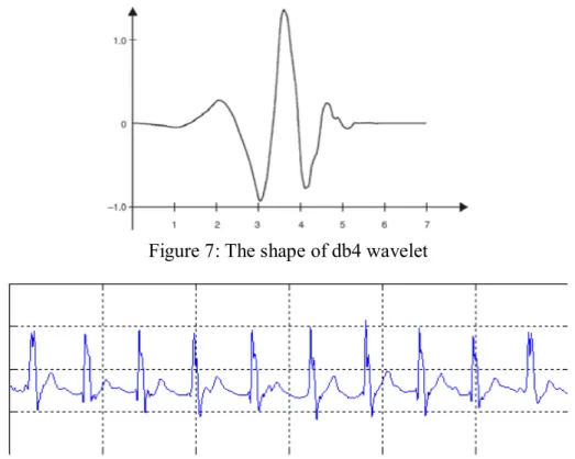
The shape of the fourth of the Daubechies wavelet family is shown in Figure 7.

Figure 7: The shape of db4 wavelet

Figure 8: Approximation signals and details of the third level of ECG decomposition of signals using db4 wavelet

Algorithm proposed by author Gyaw and Ray, also based on wavelet transformation, is based on pattern recognition (14). This algorithm consists of two phases - the learning phase and the recognition phase. Within the learning phase, a set of vectors corresponding to the wavelet transform is generated when there is R peak. This learning is done on a number of different R peaks. The recognition phase occurs when a sufficient number of such vectors have been reached. Then the ECG signal is divided into segments of fixed length, and after that the wavelet transformation is performed over it. The resulting vectors are compared with the vectors used in the learning phase. If the matching ratio is adequate, the R peak is successfully detected.

(20)

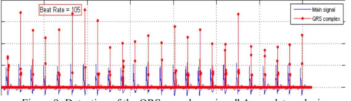
The authors Di-Virgilio and others have proposed a wavelet-oriented algorithm that divides the ECG signal into fixed-length segments (14). R peak is detected at the location since the local maxim module reaches the threshold that is previously calculated for each segment. The implementation of the wavelet-oriented algorithm for detecting the QRS complex is shown in Figure 9.

Figure 9: Detection of the QRS complex using db4 wavelet analysis

4.1.2. Wavelet based ST-segment analysis-algorithm

If there is deficiency in the blood supply to the heart muscle or no, can be detected by the changes in the ST-segment of an ECG. Also, the ST-segment may become irregular as a result of myocardial ischemia or infarction. Therefore, a precise recognition of the ST-segment including its level, has particular diagnostic importance, and usually more investigations are needed.

Sahambi and others (1998) have developed an ST-segment analysis algorithm, supported by

multi-resolution wavelet approach. It can detect the QRS complexes and analyses each beat

based on the wavelet transformation to identify the characteristic points (fiducial points) that represents iso-electric level, the J point, and onsets and offsets of the QF~S complex and T wave (15). The algorithm determines the T onset by looking for a point of inflection between the J point and the T peak.

As a result of detection of characteristic points by the wavelet technique the effect of noise can be reduced. All obtained results highlight that the projected approach provides extremely accurate ST levels, at higher heart rates and with different morphologies, opposite of the traditional (empirical) technique. The algorithm identifies the ST-segment in 92.3% beats with an error of 4ms and for 98.0% of the beats the error is within 8ms. Its accuracy is suitable within the acceptable limits of clinical environment. On-line analysis and display of ST-segment data can be provided since the algorithm has been implemented on a TMS320C25 based add-on DSP card linked to a PC.

Method

The detection of iso-electric level, onsets and offsets of the QRS and T complexes, and the J point are necessary for the detection and localization of the ST-segment. Necessary ECG data to evaluate the performance of the system are taken from two sources. First set of data is taken from a ECG simulator providing an ECG with known heart rate and ST levels. The variation in the ST levels given in a 1.0 mV ECG signal varied from -0.50 to 0.15 mV. The second set of data is taken from a sample file from the standard European ST-T database (file 'X_EDB') providing ECGs from clinical environments (15).

(21)

Detection of iso-electric level, onsets and offsets of QRS complex

The detection of iso-electric level, onsets and offset of QRS complex and T wave are provided as a result of highest total value and zero crossings of the wavelet transforms at the characteristic scales. Smoothing function O(t) with non-zero DC value (its integral is not equal to zero) may be considered as an impulse response of a low-pass filter. If smoothing function can be Gaussian and at scale a, then it can be defined such as:

θ

𝑎

(𝑡) =

1 √𝑎

θ (

𝑡

𝑎) , 𝑙𝑒𝑡

𝜓(𝑡) = (

𝑑𝜃

_{𝑑𝑡) (𝑡)}

be a function formed by the first derivative of θ(t). To detect the characteristic points, the wavelet transform of the signal is calculated. The wavelet transform of f(t) with ψ(t) as mother wavelet is defined as the inner product of f(t) with ψ*_a,t_(t).

Wf(a,τ)=( f(t), ψ

*a,t

(t))

where a is the scale parameter and τ is the shift parameter. As the wavelet is real function the conjugate of ψa,t(t) is ignored in the subsequent discussion.

𝑊𝑓(𝑎, 𝜏) =

1 √𝑎

∫ 𝑓(𝑡)𝜓 (

𝑡 − 𝜏

𝑎 )

∞ −∞

𝑑𝑡

Now:

𝜓

𝑎

(𝑡) =

1 √𝑎

𝜓 (

𝑡

𝑎)

Let

𝑡

𝑎 = 𝑢 ⇒ 𝑑𝑡 = 𝑎𝑑𝑢

Therefore

𝜓

𝑎

(𝑡) =

1 √𝑎

𝜓(𝑢) =

1 √𝑎

𝑑𝜃

𝑑𝑢 (𝑢)

And by chain rule

𝜓𝑎(𝑡) = 1 √𝑎( 𝑑𝜃 𝑑𝑡)(𝑢) 𝑑𝑡 𝑑𝑢= 𝑎 √𝑎 𝑑 𝑑𝑡𝜃 ( 𝑡 𝑎)= 𝑎 𝑑 𝑑𝑡 [ 1 √𝑎𝜃 ( 𝑡 𝑎)]= 𝑎 𝑑 𝑑𝑡 [ 1 √𝑎𝜃 ( 𝑡 𝑎)]= 𝑎 ( 𝑑𝜃𝑎 𝑑𝑡 )(𝑡)

(22)

Using t = -_{𝜏 ⇒ 𝑑𝑡 = −𝑑𝜏 in the previous eqn. we get∶}

𝛹𝑎(−𝜏) = −𝑎 (𝑑𝜃_{𝑑𝜏 )}𝑎 (−𝜏), 𝑤ℎ𝑖𝑐ℎ 𝑖𝑚𝑝𝑙𝑖𝑒𝑠 𝛹𝑎(𝑡 − 𝜏) = −𝑎 (𝑑𝜃_{𝑑𝜏 )}𝑎 (𝑡 − 𝜏) = 𝛹𝑎,𝑡(𝑡)

Considering the previous eqn. the wavelet transform can be writtenas

𝑊𝑓(𝑎, 𝜏) = 〈𝑓(𝑡), −𝑎 (𝑑𝜃_{𝑑𝜏 ) (𝑡 − 𝜏)}𝑎 〉 ⇒ 𝑊𝑓(𝑎, 𝜏) = −𝑎 (_𝑑𝜏)𝑑 〈𝑓(𝑡), 𝜃𝑎(𝑡 − 𝜏)〉

Therefore, wavelet transform Wf(a,_{𝜏) is proportional to the first derivative (w.r.t 𝜏) of}

〈𝑓(𝑡), 𝜃

𝑎

(𝑡 − 𝜏)〉 = ∫ 𝑓(𝑡)𝜃

𝑎

(𝑡 − 𝜏)𝑑𝑡

∞

−∞

In this case the zero crossing in the wavelet transform Wf(a, z), at some z = z1, match up to

the local extreme of the expression in the last equation. For proportioned waveforms such as the P wave, the zero crossing of Wf(a,τ) at some τ=τ1, among its local maxima and minima,

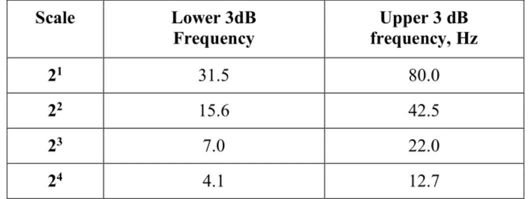
would match up to the peak of the waveform. The wavelet transforms are calculated in terms of the scales of interest. The Table 1 bellow highlights the pass bands of the wavelet filters at four scales. The outcome of base line drift and power line interference on the timing characterization and the onset of the QRS complex may be reduced by an optimized wavelet (15). Scale Lower 3dB Frequency Upper 3 dB frequency, Hz 21 _31.5 _80.0 22 _15.6 _42.5 23 _7.0 _22.0 24 _4.1 _12.7

Table 1. Pass bands of wavelet filters at four scales

Within this period the algorithm searches for 30 ms that has a minimum total value & the wavelet transform. It represents the iso-electric level. The search begin from the onset of the QRS complex and goes towards the offset of the P wave. Considering the smaller effect by base line wander looking for the iso-electric level in scale 23_{gives a further reliable value.}

Detection of S point and J point

Because of ECG composed of high frequencies around S and J point they are detected using the 21_{scale. Step behind the maxima zero crossing of Wf(2}1_{,τ) match up the S point.}

Sometimes J and S point can be same, if the J point is defined as the first inflection after the S point. After the zero crossing, first a peak for the J point is detected in scale 21_{. A search is}

conducted for a peak in a range of 20 ms after the S point in order to detect the J point. After this, the point of maximum slope is searched for. In this case The J point is distinct as the

(23)

point where the slope of Wf(21_{,τ) becomes less than 50% of the maximum slope, after the}

point at which the maximum slope occurs. In the given period if a point of inflection is not found after the S point, then the J point is used as the S point.

T onset and offset

The T wave keeps up a correspondence to a couple of modulus maxima positioned behind the end of the QRS complex with a zero crossing in between. The zero crossing among the modulus maxima provides the position of the T peak (this is true for positive and negative T waves). The first modulus maxima match up the maximum slope between the onset and the T peak while the second modulus maxima match up the greatest slope between the T peak and the offset. The search is conducted between the first modulus maxima analogous to the T wave and the QRS offset for the onset of the T wave.

Let τT1 and τT2 be the times corresponding to the first and second modulus maxima

respectively. The first modulus maxima is denoted by TP1 = Wf(23,τT1) and the second by TP2

= Wf(23_{, τ}_T2_{). Starting from τ}_T1_{, a backwards search is made for a point where Wf(2}3_{, τ}₎

satisfies any one of the following conditions:

(i) The value of Wf(23_{, τ}_{) becomes less than or equal to THP1= T}_P1_{/kp1. Here kp1 is kept}

at four.

(ii) The slope of Wf(23_{, τ}_{) changes sign (without reaching THP1).}

(iii) There is major change by the slope of Wf(23_{, τ}_).

Results

The evaluation of the algorithm is based on test data and on standard ECG data. The J point and the ST-T point are identified to check next to the calculated value. The difference among the values calculated visually and by the system represents the error.

Heart rate

min -1 Percentage of beats having error (e)ms in ST-segment length % of beats _{with error}

within 4ms

% of beats with error within 8ms

0<e<4 4<e<8 8<e<12 12<e<16 16<e<20

80 94% 5% 1% 0% 0% 94.0% 99.0%

120 90% 3% 1% 5% 1% 90.0% 93.0%

160 93% 6% 0% 0% 0% 93.0% 100.0%

File X_EDB _92% _8% _0% _0% _0% _92.0% _100.0%

Average 92.3% 98.0%

Table 2. Results of ST-segment detection with different heart rates (80/120/160)

The algorithm detects the ST-segment in 92.3% beats (Table 2) with an error of 4 ms and for 98.0% of the beats the error is within 8 ms. The accuracy of the algorithm is acceptable within the suitable limits of clinical environment.

There are possible errors due to the truth that as the heart rate moves up the T wave closer to the QRS complex. This moves the J point in terms of the T peak and the value considered is

(24)

higher (i.e. towards positive side for the case of positive T wave) than the actual value. Its consequence is extremely pronounced at 160 beats min -1. One way around this issue is to modify the value of x based on the heart rate. For example, with some values of x, the errors at 160 beats rain -t are decreased to some extent (Figure 10/c):

x=80 ms, for heart rate < 120 x=60 ms, for 120 < heart rate< 140 x=40 ms, for heart rate> t40

The J+x approach would provide inaccurate outcome, as e result of this adaption, due to its empirical nature.

Figure 10. Results of ST level calculations Jbr three values of heart rate. (a) 80," (b) 120," (c) 160 beats rain

It is obvious that the outcomes of the algorithm correspond with ordinary values exceptionally closely, as a result of determined ST-T point by detecting the inflection point between the ST-segment and the T wave but not by empirical method. For that reason there is no need any modification at this approach in terms of higher heart rates, providing additional accuracy of ST level calculation at various heart rates. The conventional approach is detected as a back-up method in case of no inflection point.

4.1.3. An algorithm for the segmentation of a waveform and algorithm for the recognition of the shape of the ST segment

SKORDALAKIS (1986) has developed a technique for the automatic identification of the ST segment considering the hypothesis that it is either a straight line or a parabola. The outcomes of this process used to a certain ST segment are:

a) The values of the onset and of the end of this ST segment and

b) The equation of a straight line or of a parabola that best approximates this ST segment The Algorithm for the Segmentation of a Waveform could be described as follows:

(25)

Start:

Step l: use couples of adjacent segments in the order (S1, S2), (S3, S4), since Si represents the

segment i (supposing a left to right numbering of them) and adjust the middle point of every couple following the procedure for adjusting the middle point of a couple of segments;

Step2: use couples of adjacent segments in the order (S2, S3), (S4, S5) and adjust the middle point of each pair of segments as in step l;

Step3: if no pair of adjacent segments was adjusted in step l and step 2 then stop else got d- step l;

End.

The Algorithm for the Recognition of the Shape of the ST Segment

The following modifications were made to the above algorithm. 1. The quantity of segments is limited to three.

2. The preliminary segmentation is (ib, im1, im2, ie) since ib is the initial sample point of

the auxiliary segment,

ie - is the last sample point of the auxiliary segment.

im1 = ib + (ie - ib)/3,

im2 = im1 + (ie - ib)/3.

3) The data of all three segments S1, S2, S3, are approximated by the functions fk1 (x), fk2 (x),

fkl (x), correspondingly since is not necessary for the functions fkl (x), fk2 (X), fk3 (x), to be the

same function. Furthermore the algorithm has been implemented four times for measuring four segmentations of the auxiliary segment. Each moment, as functions fkl (x), fk2 (X), fk3

(x), k = 1(1) 4, the ones shown in Table 3 have been implemented.

k J

f

k1

(x)

f

k2

(x)

f

k3

3

x+b

3

x

As the best segmentation inside all four segmentations of the auxiliary segment is used the one with the smallest error norm. The second segment represents the ST segment.

Peng and Wang (2016) have confirmed that using their proposed method, the signal analysis and processing may be separated into two steps as direct and transformation analysis. Implementation of this method may reduce the time for transformation, so useful signal loss can be reduced, and accuracy of detection increased (17).

(26)

Signal transformation analysis and processing is performed into wavelet transformation or EMD transformation by mapping the signal to another domain (18).

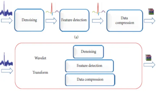
ECG signals processing of usual processes, including denoising, feature recognition, and filtering of the three major procedures are presented at Figure 11/a. In case of _{n is the} duration of the signal under standard conditions, each process needs to undertake a conversion, considering that each transformation obtains a time frequency of _{T0(n) = C0 n2.} Supported by these circumstances, denoising, detection, and compression have been performed. Considering that the time frequency of each procedure is _{T1(n) = C1n, the entire} period necessary for the conventional signal processing method is 3(T0(n)+T1(n)) =

3(C0n2+C1n).

Figure 11: Comparison of two different algorithms for ECG signals processing.

If the projected algorithm has been implemented for completing the denoising, the detection, and the compression operation, the entire procedure only needs to perform the wavelet transform one time, with a period taken of T0(n) + 3T1(n) = C0n2+3C1n ( Figure 11/b). Developed algorithm may decrease the period for transformation between signal domains as a result of the mix of feature detection, signal filtering, and signal compression, providing resources and speeding up the activities (18). As the wavelet transformation needs to follow both activities of decomposition and reconstruction, the useful signal is frequently lost during the process of conversion.

The wavelet transform has been implemented by Peng and Wang in order to gain wave trapping extraction, to remove the feature signal component from wavelet decomposition signal. Their technique provides the feature location, signal filtering, signal compressing and other processing, providing reduction of computing resources, speed up the processing, and improve the detection accurateness.

(27)

4.1.4. An algorithm for ST shape analysis

In order to avoid the progress of heart disease and sudden death, Jeong and others (2010) have designed a small-size (76mm by 59mm) ECG device, providing safety and efficient monitoring. Such system could recognize the temporary change of ECG which is very important to diagnose heart disease such as myocardial ischemia, arrhythmia and cardiac infarction (4). Using LabVIEW program, the major role of the software is to detect the feature points, ST-segment level and shape.

The ST segments have been classified by their morphology in order to detect the transient changes of ST. At the beginning a pair of reference ST shapes is given. Included ECG analysis algorithm analysis consists of feature point detection and ST shape classification. Within the procedure of feature point detection S wave and J-point detection have been performed, and the proposed algorithm classifies the STs into reference ST shapes. The rules for the trend of prior beats and the shape category of prior beats have been implemented in order to develop the performance of ST shape categorization.

Detection of feature points

Supported by searching method based on the R peak there is a detection in terms of the feature points like PR level point, J-point, S wave, etc. as a. (a) and (b).The establishment of detection area for discovering S, Q and T wave has been shown in Fig 12. The duration of the Q wave detection area is 160ms.

In general, the PR interval is 120ms to 200ms since the time of 160ms contains the period of the P wave. For that reason 160ms consist of 50% of the period of QRS complex and the beginning of the Q wave. The Q wave detection area has been divided into four parts as shown in Fig 1(c) providing the minimum point or the inflection point as Q wave. Step behind Q wave detection, PR level point has been identified by discovering the inflection point around for Q wave. On the same method S wave, used in Q wave detection as shown in Fig. 12(d). J-point has been identified by finding the inflection point around for S wave.

Calculating ST level

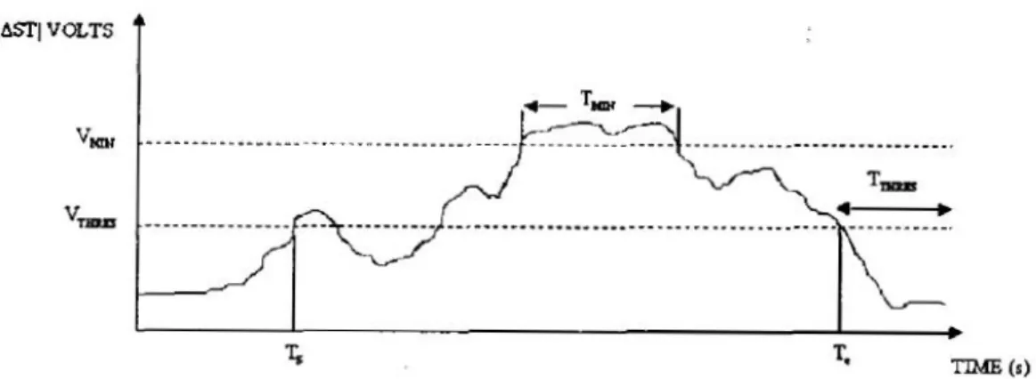
Based on the definition of ST episodes in the European ST database, the ST level has been calculated. 80ms after the J-point ST segment deviation has been measured but the heart rate had not exceeded 120 bpm. 60ms after the J-point the ST segment deviation has been measured but the heart rate had exceeded 120 bpm. The start of an ST level episode is positioned by looking backward from the time since the total ST deviation first exceeds 0.1mV until a beat is found, for which the total ST deviation is less than 0.05mV. The variation that does not preserve its level for 5sec to construct a continuous section of ST level change has been unnoticed (4). The end of an ST level episode is positioned by searching forward from the period since the total ST deviation last exceeded 0.1mV until a beat is found, for which the total ST deviation is less than 0.05mV. At least 30sec, ST episode section has to keep the total ST deviation no less than 0.1mV

(28)

Figure 12. Detection of feature points

ST shape classification

By match up the four slopes of an ST in ECG data with those in the reference set ST shape classification in ECG data has been conducted. Supported by the four slopes, it has been easy to differentiate among concave, convex and negative-T type, and it has been easy to differentiate these categories from up-sloping, horizontal and down-sloping. The major issue is to make a distinction among up-sloping, horizontal and down-sloping, as a result of the difference among these categories is only the slope in the middle section (4).For that reason, a rule set for improving the performance of ST shape classification among up-sloping, down-sloping and horizontal has been established. All results of the ST shape classification have been shown in Fig 13-16.

(29)

Figure 13. STs of concave type

(30)

Figure 15. STs of up-sloping type

(31)

Supported by LabVIEW program ECG analysis software that has been developed for Holter analyzer is shown in Fig 17. The software presents all results from ECG shape classification. Also ST level has been displayed below ECG signal. The information of ST shape and ST level change can be provided from the window.

Figure 17. Portable ECG device

An instrumentation amplifier, filter, micro-controller and transmitter module have been included in the portable ECG measurement device. Fig. 18 shows the Hardware configuration of ECG measurement device.

Figure 18. Hardware configuration of ECG device

4.1.5. ST (change detection) analysis algorithm

Most of the algorithms that have been developed until now place importance on the detection of the ST level change, but the classification of the ST shape has been from key importance for Jeong and Yu (2007) in terms of monitoring a preventing of ischemia such as cardio disease. A small-size portable ECG device and a suitable developed algorithm detects the ST level changes have been designed by Jeong and Yu.

The STs have been classified into seven categories by comparing the slope values of the STs and ones of the reference STs with proposed algorithm (19). All analysis results present the data in terms of ST level change and ST shape change that could be implemented by cardiologists to analyze ST-T episodes.

The algorithm designed for ST change detection funds the least squares curve for the data between S wave and T wave in ECG considering that the least square curve for ST has been of importance to notice the change of ST shape. The change of ST shape has been detected

(32)

by comparison among pseudo STs that is the approximate curve of the original ST. The ECG has been analyzed by the algorithm automatically and has been noticed irregular part in ECG. All results have been implemented to provide control signal that decides about the start and the end of ECG recording since the device provides the delivers ECG data of recorder to PC (19).

Configuration of reference STs

Commonly, there are concave, convex, horizontal, down-sloping and up-sloping ST shapes. Fig. 19 represents the reference ST types. In the figure, (+), (0) and (-) mean the sign of the slope value in the ‘|↔|’ marked points.

Figure 19. Reference STs

The proposed algorithm locates the least square curve between the S and T wave step behind the recognition of the QRS complex and T wave in a test ECG. The four slope values have been measure from the least square curve for comparison with those of the reference ST types. The first and the fourth slope values show the permanence of the S wave and the appearance of the T wave, correspondingly. Therefore, since the S wave exists, the first slope value is positive as a result of the positive slope directly after the lowest point of the S wave. Also, the fourth slope has a positive value since the T wave is positive and is negative if the T wave is negative.

The slope value in the middle of RR interval has been selected as the fourth slope value in case of no T wave. Usually, the third slope value has been extracted in the middle between the fourth point and J-point, as a result of feature points detection, but if the minimum point with a zero slope value exist around the middle between the first and the fourth point as shown in (d) and (e) of Fig. 19, that point is selected as the third point.

(33)

In the middle of the J-point and the third point the second slope value is extracted. No S wave is common to types (a), (e) and (f). The distinction among these types is that kind (a) has only positive slope values after the zero slope point, and kind (e) has both positive and negative slope values before or after the zero slope point, and kind (f) has only negative slope values. All slope values are positive in the case of type (b) while the slope value stays at zero for some instance in the case of type (c). Type (d) varies from type (e) consider type (d) has an S wave. The proposed algorithm classifies STs within seven classes (a), (b), (c), (d), (e), (f) and (X). All additional ST shapes besides the ST shapes exposed in (a) to (f) are classified as type (X). Upslopping depression and concave elevation frequently are without any implication in many cases while down-sloping depression and convex elevation are very important as same as ST depression such as (e). The outcome of distinguishing an ischemic ST from a non-ischemic one is expected to be improved as a result of the ST shape classification (19).

Polynomial approximation

Within the analysis of the ST shape, the original ECG data has not been used. The real ST data must be interpolated in order to provide calculation of the variation of the ST shape. The interpolation such as process can reduce the noise in the original ECG representing a low-pass filter. Two techniques to approximate ST into a polynomial formula have been implemented. One is to approximate ST into one polynomial formula of 9th order over the entire ST. The second one is to approximate ST into three polynomial formulas of under 5th order for the three-segmented ST. The one of the two ways is chosen due to the magnitude of the noise in ST (19).

ST shape classification

Within the classification procedure have been used the reference ST types. During the ST shape classification, the values of slopes have been implemented in order to be extracted from the reference ST types. The proposed algorithm implements the slope values of the four points in the section between the S and T waves in order to classify the ST shape type. According to the slopes the four points of the measured ST, have been classified by the algorithm. Fig. 20 represents the ECG analysis process. The first procedure is to detect the feature points such as the QRS complex, J-point, etc. After that, the proposed algorithm discovers the ST level change. ST shape classification is not applied to all ECG data. Its procedure is implemented just to the segments including the ST level change episodes. All ending results of the analysis offer data about both the ST level change and ST shape type that are implemented in the ST level change section (19).

(34)

Figure 20. ECG analysis process

4.1.6. Algorithm based on ST morphological change (ST shape classification) Jeong and others (2010) have concluded that the crucial step in identifying myocardial ischemia is to locate the start of the ST level change in the entire ECG and the second crucial step is to verify ST level variation and morphological ST change while finding the end of the ST level change (5).

Therefore, Jeong and others paid particular attention to the morphological ST change and on building an algorithm for ST shape categorization. As it is mentioned above, STs are usually divided into five morphologies: up-sloping, down-sloping, horizontal, concave, and convex.

Morphological classification of ST

ST shape classification in ECG data has been performed by comparing the four slopes of an ST in ECG data with those in the reference set. Using the four slopes, it was easy to distinguish among the concave, convex and negative-T types, and easy to distinguish these types from up-sloping, horizontal, and down-sloping. The main issue is how can we distinguish among up-sloping, horizontal, and down-sloping, because the difference among these types is only in the slope in the middle region. For that reason, a rule set for strengthening the features of ST shape categorization among up-sloping, down-sloping, and horizontal have been developed and implemented supported by several parameters as follows:

(35)

(1) p(%): rate of a flat region in between the J-point ant T peak.

(2) θ(rad): mean of slope value in the flat region.

(3) s(rad): trend of slope for the previous two beats.

(4) t: trend of shape for the previous two beats.

The slope angle of the second point in ST that has been classified in the horizontal type has been monitored. The slope angle of the second point is less than 0.02 rad (about 1.15◦) for ST to be classified as a horizontal type while the amount of the part where the slopes are less than 0.02 rad to the entire ST part is almost 27.5%. Commonly, the standard QT period between the Q and T wave counts 370 ms, and the period of a normal QRS complex counts 80ms at 70 beats per minute (bpm). The period of the T wave counts 250 ms. The period of a normal ST could be measured at 40ms which accounts for about 25% of the interval between as a result of the common period of the QT interval, QRS complex, and T wave at 70 bpm the J-point and T peak. 0.02 rad, 27.5%, and 25% have been implemented as basic factors for building the four parameters comprising the rules. The first parameter has the period p (%) since the slope angle is up-holded on less than 0.02 rad (about 1.15◦_{) in between the J point}

and T peak, that clearly designates the correspondences among the horizontal shape in the reference STs and the ST shape of the present beat p has been classified into three sets, highlighted by

S={ p|22.5 > p} M={ p|22.5 ≤ p ≤ 27.5}

L={p|27.5 < p}

The next parameter represents the mean slope value θ(rad) of the period whose slope has been established at less than 0.02 rad, clearly indicating the correspondences among the horizontal shape in the reference STs and the ST shape of the present beat. As parameter it can be categorized into three sets as follows:

N ={θ| - 0.0087 > θ} CE ={θ| - 0.0087≤ θ ≤ 0.0087}

P ={θ| 0.0087 < θ}

The trend of slope s(rad) represents its parameter indicating the trend for the ST slope change. The total of the slope values of the previous two beats is the value s (rad). CE has been implemented including the slope variation of 0.02 rad downward in the previous two beats, since the categorized value s into three sets is represented by

N ={s| - 0.01 > s} CE ={s| - 0.01 ≤ s ≤ 0.01}

P = {s| 0.01 < s}

The fourth parameter is the score t of the determined shape type of the previous two beats and represents the trend of the ST shape change. The shape trend parameter t is the sum of each

(36)

score of the two previous beats and is classified into two sets represented by

L = {t| 0.85 > t}

H = {t| 0.85 ≤ t}

The result is given by multiplying K (the value assigned to each ST shape) and W (the weighting factor). K was assigned to be 0.5 for the horizontal shape, 0.4 for the down-sloping and up-sloping shapes, 0.3 for the concave shape, and 0.2 for the convex and negative-T shapes (5). The K value increases if the ST of the previous beat is more similar to horizontal type. If the STs of the earlier two beats were analogous to the horizontal type, there is huge possibility that the ST type of the current beat had been horizontal.

The weight feature depends of the slope value of ST and is represented by:

𝑊(𝜃) {0.9

_{5|𝜃| + 1 |𝜃| ≤ 0.02(𝑟𝑎𝑑)}

|𝜃| > 0.02(𝑟𝑎𝑑)

In order to provide the best characteristics of distinctive among up-sloping, horizontal, and down-sloping, 0.85 has been determined as the margin between L and H sets. In order to configure N, CE and P sets 0.0087 has been used as θ.

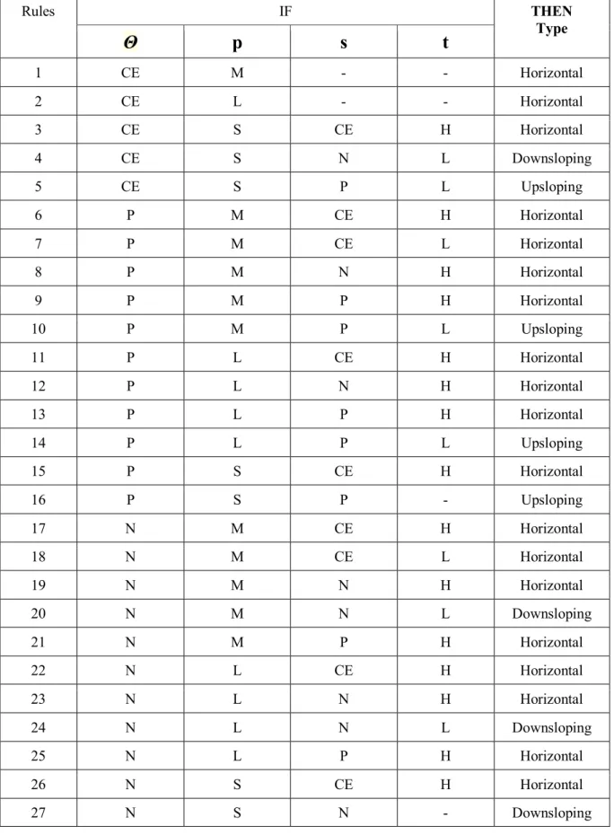
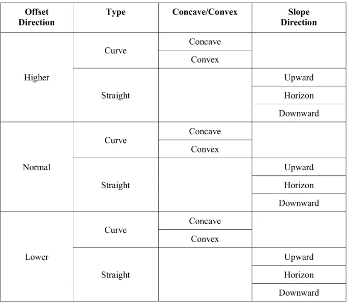
As shown in Table 6, supported by the sets of p, θ, s, and t, 27 rules have been developed, produced from an iteration procedure for adjusting parameters and applied to test ECGs, and the results have been calculated. All 27 rules are implemented in the categorization between up-sloping, horizontal, and down-sloping shapes after the end of the ST classification procedure implementing the four slope values. Because the rules have already been implemented to provide better performance of classification among the up-sloping, horizontal, and down-sloping types, authors have implemented the parts of the test ECG to establish the rules (5).

In Table 4, ‘–’ correspond to all conditions. For example, when is a part of CE and p is a part of M or L, the ST is determined as a horizontal shape for all s and t. When ST is not categorized by the rules, the outcome of the ST shape classification maintains the shape by ST categorization using four slopes.

(37)

Rules IF THEN Type

Θ

p

s

t

1 CE M - - Horizontal 2 CE L - - Horizontal 3 CE S CE H Horizontal 4 CE S N L Downsloping 5 CE S P L Upsloping 6 P M CE H Horizontal 7 P M CE L Horizontal 8 P M N H Horizontal 9 P M P H Horizontal 10 P M P L Upsloping 11 P L CE H Horizontal 12 P L N H Horizontal 13 P L P H Horizontal 14 P L P L Upsloping 15 P S CE H Horizontal 16 P S P - Upsloping 17 N M CE H Horizontal 18 N M CE L Horizontal 19 N M N H Horizontal 20 N M N L Downsloping 21 N M P H Horizontal 22 N L CE H Horizontal 23 N L N H Horizontal 24 N L N L Downsloping 25 N L P H Horizontal 26 N S CE H Horizontal 27 N S N - Downsloping

A survey of algorithms for ischemia detection in ECG recordings

Politecnico di Milano

Polo di Como

Scuola di Ingegneria dell’Informazione

Corso di Laurea Specialistica in Ingegneria Informatica

A Survey of Algorithms for Ischemia

Detection in ECG Recordings

Tutor universitario:

Elaborato finale:

Prof. Giuseppe Pozzi

Mario KOSTOSKI, matr. 864445

Dr. Rodolfo Pizzuto

Table of Contents

Abstract

Sommario

1. Introduction

1.1. Tesina outline

2. Source selection

3. Taxonomy of algorithms

3.1. The heart’s structure

3.2. Ischemia as a cardio disease

3.3. Ischemia detection with ECG

3.4. Software detection of the QRS complex

3.5. Description of the algorithms

(𝑆𝑇_𝑆𝑒 =

𝑇𝑃 + 𝐹𝑁)

𝑇𝑃

(𝑆𝑇_𝑃 =

𝑇𝑃 + 𝐹𝑃)

𝑇𝑃

(𝐼𝑆_𝑆𝑒 =

𝐼𝑆

𝐼𝑆

(𝐼𝑆_𝑃 =

𝐼𝑆

𝐼𝑆

+ 𝐼𝑆

)

4. The algorithms

4.1. Algorithms based on wavelet transformation

𝑊𝑓(𝑎, 𝑏) = ∫ 𝑓(𝑡)Ψ

(𝑡)𝑑𝑡

Ψ

(t) =

1

√2

Ψ (

𝑡 − 𝑏

𝑎 )

𝑊𝑓(2

, 𝑏) = ∫ 𝑓(𝑡)Ψ

(𝑡)𝑑𝑡 ,

𝑤ℎ𝑒𝑟𝑒

Ψ

(𝑡) =

1

2

Ψ (

𝑡 − 𝑏

2

)

Method

Detection of iso-electric level, onsets and offsets of QRS complex

θ

(𝑡) =

1

√𝑎

θ (

𝑡

𝑎) , 𝑙𝑒𝑡

𝜓(𝑡) = (

𝑑𝜃

𝑑𝑡) (𝑡)

Wf(a,τ)=( f(t), ψ

(t))

𝑊𝑓(𝑎, 𝜏) =

1

√𝑎

∫ 𝑓(𝑡)𝜓 (

𝑡 − 𝜏

_{𝑇𝑃 + 𝐹𝑁)}

_{𝑇𝑃 + 𝐹𝑃)}

_𝐼𝑆

_𝐼𝑆

_{(𝑡)𝑑𝑡}

_{, 𝑏) = ∫ 𝑓(𝑡)Ψ}

_{𝑑𝑡) (𝑡)}