Degree in Economics
Title:
Allyn, A Recommender Assistant for Online Bookstores Author: Laia Esquerrà Schaefer
Statistics Advisor: Esteban Vegas Lozano
Department: Genètica, Microbiologia i Estadística, secció d’Estadística
Economics Advisor: Dr. Salvador Torra Porras
Department: Econometria, Estadística i Economia Espanyola Academic year: 2017-18
Universitat de Barcelona
Double Bachelor Degree in Statistics and
Economics
Bachelor’s Degree Thesis
Allyn: A Recommender Assistant for Online
Bookstores
Laia Esquerrà Schaefer
June 2018
Statistics Advisor: Esteban Vegas Lozano
Economics Advisor: Dr. Salvador Torra Porras
Facultat de Matemàtiques i Estadística
Facultat d’Economia i Empresa
Recommender Systems are information filtering engines used to estimate user preferences on items they have not seen: books, movies, restaurants or other things for which individuals have different tastes. Collaborative and Content-based Filtering have been the two popular memory-based methods to retrieve recommendations but these suffer from some limitations and might fail to provide effective recommendations. In this project we present several variations of Artificial Neural Networks, and in particular, of Autoencoders to generate model-based predictions for the users. We empirically show that a hybrid approach combining this model with other filtering engines provides a promising solution when compared to a standalone memory-based Collaborative Filtering Recommender. To wrap up the project, a chatbot connected to an e-commerce platform has been implemented so that, using Artificial Intelligence, it can retrieve recommendations to users.
Keywords: Recommender systems, Collaborative filtering, Artificial neural networks,
Denoising autoencoders, KerasR, Tensorflow, E-commerce, Information retrieval, Chatbots
AMS Classification (MSC2010): 62M45 Neural nets and related approaches
Els Sistemes de Recomanació són motors de filtratge de la informació que permeten estimar les preferències dels usuaris sobre ítems que no coneixen a priori. Aquests poden ser des de llibres o películes fins a restaurants o qualsevol altre element en el qual els usuaris puguin presentar gustos diferenciats. El present projecte es centra en la recomanació de llibres.
Es comença a parlar dels Sistemes de Recomanació al voltant de 1990 però és durant la darrera dècada amb el boom de la informació i les dades massives que comencen a tenir major repercussió. Tradicionalment, els mètodes utilitzats en aquests sistemes eren dos: el Filtratge Col·laboratiu i el Filtratge basat en Contingut. Tanmateix, ambdós són mètodes basats en memòria, fet que suposa diverses limitacions que poden arribar a portar a no propocionar recomanacions de manera eficient o precisa.
En aquest projecte es presenten diverses variacions de Xarxes Neuronals Artificials per a generar prediccions basades en models. En concret, es desenvolupen Autoencoders, una estructura particular d’aquestes que es caracteritza per tenir la mateixa entrada i sortida. D’aquesta manera, els Autoencoders aprenen a descobrir els patrons subjacents en dades molt esparses. Tots aquests models s’implementen utilitzant dos marcs de programació: Keras i Tensorflow per a R.
Es mostra empíricament que un enfocament híbrid que combina aquests models amb altres motors de filtratge proporciona una solució prometedora en comparació amb un recomanador que utilitza exclusivament Filtratge Col·laboratiu.
D’altra banda, s’analitzen els sistemes de recomanació des d’un punt de vista econòmic, emfatitzant especialment el seu impacte en empreses de comerç electrònic. S’analitzen els sistemes de recomanació desenvolupats per quatre empreses pioneres del sector així com les tecnologies front-end en què s’implementen. En concret, s’analitza el seu ús en
chatbots, programes informàtics de missatgeria instantània que, a través de la Intel·ligència
Artificial simulen la conversa humana.
Per tancar el projecte, es desenvolupa un chatbot propi implementat en una aplicació de missatgeria instantània i connectat a una empresa de comerç electrònic, capaç de donar recomanacions als usuaris fent ús del sistema de recomanació híbrid dut a terme.
Paraules clau: Sistemes de recomanació, Filtratge Col·laboratiu, Xarxes Neuronals
Artificials, Denoising autoencoders, KerasR, Tensorflow, Comerç electrònic, Recuperació d’informació, Chatbots
Classificació AMS (MSC2010): 62M45 Neural nets and related approaches
First, I want to thank my statistics advisor, Esteban Vegas, for all the time spent giving me useful advice, for encouraging me to overcome the difficulties I encountered during the realization of this work and for all the work he has put to work with me with the never ending changes there have been since we first started to talk about it last year.
Second, my economics advisor, Dr. Salvador Torra, for the help and ressources provided not only for the economic analysis but also for the statistics part.
About a year ago I was introduced to Recommender Systems in a short summer course. It was most definitely a fascinating topic for me and one thing became clear: I would do my Bachelor’s Thesis dedicated to it. Therefore I also want to thank Bartek for introducing this topic in his course although he might not remember me and not even be aware of what has come out of it.
Furthermore, I want to thank Ernest Benedito, for introducing me to chatbots and for always being open to collaborate, offering his support throughout the project.
Finally, I would like to thank my family and close friends that have offered their support during the realization of this work and the completion of the Degree, with the special mention of Sandra and Marc, who have been following the progress of it and offered their help in many occasions.
List of Figures
vi
List of Tables
vii
List of Abbreviations
viii
Notation
ix
Introduction
1
Methodology
5
1 Recommender Systems 5 1.1 Data Sources . . . 6 1.2 Recommendation Techniques . . . 112 Artificial Neural Networks 17 2.1 Precedents . . . 20
2.2 Elements of an Artificial Neural Network . . . 22
2.3 Variants of Artificial Neural Networks . . . 31
2.4 Parameter and Hyperparameter Tuning . . . 35
2.5 Programming Frameworks . . . 36
3 Chatbots 39 3.1 Building blocks . . . 40
I An Economic Analysis
44
4 State of the Art Recommender Systems 45
4.1 Current applications in the Market . . . 46
4.2 E-commerce and Recommender Systems . . . 48
4.3 Causal Impact on Revenues . . . 51
5 Actual Use Cases 54 5.1 Amazon.com . . . 54 5.2 Netflix . . . 56 5.3 YouTube . . . 58 5.4 LinkedIn . . . 61
II Implementation
63
6 The Dataset 64 6.1 Data Enrichment . . . 66 6.2 Data Preprocessing . . . 68 6.3 Dimensionality reduction . . . 72 7 Back-End Development 75 7.1 Experimental Framework . . . 76 7.2 Model Variations . . . 817.3 Filtering and Recommendation Phase . . . 85
7.4 Setting Up Accessible Files and Models . . . 86
8 Front-End Implementation 90 8.1 Chatbot Creation . . . 91
8.2 Bot API Requests . . . 93
8.3 Answer formats . . . 93
8.4 Retrieving Recommendations . . . 94
Conclusions
97
9 Conclusions and Future Work 97 9.1 Conclusions . . . 989.2 Contributions . . . 99
Appendices
103
A Auxiliary Data 103
A.1 ANOVA Test Values for Clusters . . . 103
A.2 ANOVA and Tukey’s HSD Test Values for Models . . . 109
A.3 ANN Training Figures . . . 114
B R Code 119 B.1 Preprocessing . . . 119
B.2 Webscraping . . . 124
B.3 Clustering and Profiling . . . 126
B.4 Artificial Neural Network . . . 130
B.5 Chatbot . . . 137
2.1 Biological Neuron vs. Perceptron. Source: Cheng and Titterington (1994) 20
2.2 Single Hidden Layer ANN . . . 22
2.3 Identity Transformation . . . 24
2.4 Threshold Transformation for ◊ = 0 . . . 24
2.5 Softmax Transformation . . . 24
2.6 ReLU Transformation . . . 25
2.7 Tanh Transformation . . . 25
2.8 MLP Structure . . . 26
2.9 Gradient Descent Learning Rates . . . 29
2.10 LeNet-5 5-layer CNN for Optical Character Recognition . . . 32
2.11 Folded and Unfolded Basic RNN . . . 33
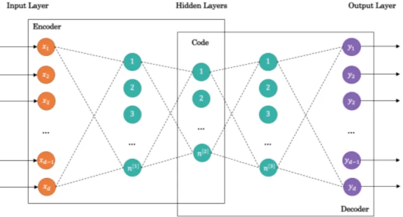
2.12 Structure of an Autoencoder with 3 Fully-Connected Hidden Layers . . . . 34
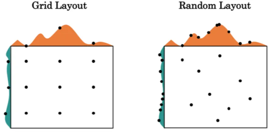
2.13 Grid-layout vs Random Seach . . . 36
2.14 Coarse to Fine Search . . . 36
2.15 Single Layer ANN . . . 37
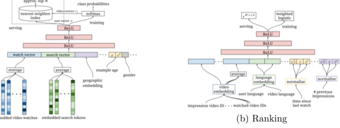
4.1 Recommendation System Architecture Demonstrating the Funnel where Candidate Videos are Retrieved and Ranked before Presenting only a few to the User. Source: Covington, Paul et al. (2016) . . . 48
4.2 Outgoing Co-purchase Suggestion for a Cookware Product sold on Ama-zon.com. Source: Amazon.com . . . 50
4.3 Outgoing Co-purchase Suggestion for a Book sold on Amazon.com. Source: Amazon.com . . . 50
5.1 Deep Neural Networks Structure for YouTube’s RS. Source: Covington, Paul et al. (2016) . . . 60
6.1 Relative Frequences of the Top 10 Cities . . . 66
6.2 Relative Frequences of the Top 5 Countries . . . 66
6.3 Years of Publication . . . 70
6.4 User Ages . . . 70
6.5 Book Ratings . . . 71
6.7 Cluster Conditional Distribution for Numerical Variables . . . 73
6.8 Conditional Continent Distribution . . . 73
6.9 Conditional Genre Distribution . . . 74
7.1 Training Accuracy per Iteration on 3 Layer Autoencoders with 256-16-256 Hidden Units using Different Optimization Algorithms . . . 77
7.2 Random Search for Initial Hyperparameter Tuning. Bigger points represent higher accuracies at iteration = 50 . . . 79
7.3 Train and Validation Accuracy History for M2 . . . 80
7.4 Training Accuracy per Iteration and Mini Batch on 1 Layer Autoencoder with 256 Hidden Units, Gaussian Noise and External Variables . . . 83
7.5 Diagram of the Data Structure . . . 87
8.1 Bot Initialization Page . . . 92
8.2 Bot’s Guided Dialog Answer Tree . . . 94
8.3 Bot Reply Keyboard Markup Examples . . . 95
9.1 Training and Validation Accuracy per iteration on 1 layer Denoising AE on 5166 users . . . 100
A.1 H1 Training and Validation History . . . 114
A.2 H2 Training and Validation History . . . 114
A.3 H3 Training and Validation History . . . 115
A.4 H5 Training and Validation History . . . 115
A.5 H7 Training and Validation History . . . 115
A.6 H4 Training and Validation History . . . 115
A.7 H6 Training and Validation History . . . 115
A.8 H8 Training and Validation History . . . 115
A.9 M1 Training and Validation History . . . 116
A.10 M3 Training and Validation History . . . 116
A.11 M2 Training and Validation History . . . 116
A.12 M4 Training and Validation History . . . 116
A.13 M5 Training and Validation History . . . 117
A.14 M7 Training and Validation History . . . 117
A.15 M9 Training and Validation History . . . 117
A.16 M6 Training and Validation History . . . 117
A.17 M8 Training and Validation History . . . 117
A.18 M10 Training and Validation History . . . 117
A.19 Gaussian Noise Training and Validation History . . . 118
A.20 Lit & Fict. Training and Validation History . . . 118
2.1 Statistics vs. Machine Learning Terms . . . 19
6.1 Example of a Repeated Book Title . . . 69
6.2 Final Merged Book Genres . . . 69
6.3 Sample of Books Read by Users Under 5 Years Old . . . 71
6.4 Sample of Books for 5 Year Olds . . . 71
7.1 Baseline Model Results . . . 75
7.2 1 Hidden Layer Autoencoders Performance . . . 79
7.3 Performance Improvement Adding Dropout to the 1 Layer Autoencoder with 64 Hidden Units . . . 81
7.4 Performance Improvement Adding Dropout to the 1 Layer Autoencoder with 256 Hidden Units . . . 81
7.5 Performance Comparison for Genre Specific AE . . . 84
AE Autoencoder
AI Artificial Intelligence
ANN Artificial Neural Network
API Application Programming Interface
BX Book-Crossing
CB Content-based
CF Collaborative Filtering
CNN Convolutional Neural Network
DNN Deep Neural Network
DL Deep Learning
GLM Generalized Linear Model
KB Knowledge-based
LP Long Polling
MAE Mean Absolute Error
ML Machine Learning
MLP Multilayer Perceptron
NCAE Neural Collaborative Autoencoder
NL Natural Language
NLP Natural Language Processing
NLU Natural Language Understanding
RMSE Root Mean Square Error RNN Recurrent Neural Network
RS Recommender System
General v scalar value v row vector vT column vector M matrix ‡x standard deviation of x
covariance matrix of x and y
Cumulative Distribution Function (CDF) of the standard nor-mal distribution
Sizes
d total number of input nodes
L number of layers in the network
m number of examples in the dataset
n[l] number of hidden units (nodes) of the lth layer
ny output size (or number of classes)
Objects
X œ IRd◊m input matrix
x(i) œ IRd ith example represented as a vector, i = 1...m xj œ IR1 jth input node, j = 1...d
Y œ IRny◊m label (output) matrix
y(i) œ IRny output label for the ith example, i = 1...m. It can also be a
vector, y(i), when n
ˆy(i) œ IRny predicted output value for the ith example, i = 1...m. It can
also be a vector, y(i), when n
y >1 yj œ IR1 jth output node, j = 1...ny
a[l] activated value of the hidden units of the lth layer
b[l] bias vector of the lth layer
W[l] weight matrix of the lth layer
z[l] input value of the hidden units of the lth layer
Functions
‡(z) activation function
L(ˆy, y) loss function
"People read around ten MB worth of material a day, hear 400MB a day, and see one MB of information every second" - The Economist (November 30, 2006)
That was in 2006. Almost 12 years after, this volume has increased by a factor of 28
according to Moore’s Law: 5GB worth of material read and 100GB heard a day; 512MB of information seen every second. We are talking about massive volumes of data, which have become impossible to process by humans.
The Paradox of Choice defines how having too many options is actually
counterpro-ductive. Furthermore, this data overload not only affects users, but also companies who have faced difficulties to extract relevant information from it.
Through Machine Learning and Recommender Systems, we can overcome these. Both research fields have been developing high performance technologies and algorithms to process massive data which have given rise to automated information filtering engines.
Nevertheless, most of these algorithms face several problems; the most relevant being
data sparsity. This means that when trying to provide suggestions to a user for example,
only a few other users might have common elements in their past review history. Without common information, measuring similarities and providing suggestions for items of use becomes a hard task. Hybridization methods combining several techniques try to deal with these deficiencies.
This Thesis is developed with the objective of getting a better insight on Recommender Systems and provide an end-to-end solution that integrates an algorithm or an hybridized combination able to compute accurate rating predictions.
Aim of the Project
The main goal of this project is to get deeper insights on Recommender Systems using Artificial Neural Networks, two areas in Statistics which haven’t been seen in depth during the Bachelor’s Degree. As part of this project, we develop a detailed guide to these study areas.
Furthermore, we want to provide an end-to-end solution, where recommendations can be retrieved by any user at any time. These kind of solutions are quite infrequent in the field of Recommender Systems, as companies who have developed them focus on the integration of these algorithms in their websites. Therefore, we develop an open real-time solution which opens the door for possible future works, a Chatbot (also refered as Bot). Through the development of this Thesis, we pretend to accomplish the following goals: • Provide a general overview on the current state of Recommender Systems and
their penetration in e-commerce platforms.
• Define the most common data structure used to develop Recommender Systems, and specially the challenges it represents for traditional Statistics.
• Present a general overview on Artificial Neural Networks, how they relate to Statistics and their role in Recommender Systems.
• Implement a Neural Recommender System able to provide accurate predictions for new users.
• Introduce the concept of Chatbot and its role as a real-time Recommender Assistant. • Implement the Chatbot in a front-end application to make the system reachable
for potential users.
Scope
In order to limit the scope of this project to the magnitude of the Bachelor’s Thesis, the knowledge domain is contrained to online bookstores, and more specifically to the recommendation of Adult Books. The focus is set on retrieving accurate predictions without letting the front-end solution aside, which is presented as a simple Proof of Concept where we test its potential functionalities.
Report Outline
This report consists of nine chapters additionally to this Introduction where the project is introduced. Chapters are split into several parts:
• Methodology
– Chapter 1: Recommender Systems. An introduction to Recommender
Systems is provided, detailing data sources and recommendation techniques used.
– Chapter 2: Artificial Neural Networks. We provide deep insights on this
set of techniques, building the algorithm from the ground up.
– Chapter 3: Chatbots. We expose a brief historical introduction to Chatbots
and define their main building blocks. A state of the art analysis on the use of Chatbots for Recommender Systems is provided
• Part I: An Economic Analysis
– Chapter 4: State of the Art Recommender Systems. We define present
and potential applications of Recommender Systems and discuss their impact measures.
– Chapter 5: Actual Use Cases. The Recommender Systems implemented
by four specific companies are detailed. • Part II: Implementation
– Chapter 6: The Dataset. We introduce the set of data available to train
the system.
– Chapter 7: Back-End Development. The experiments developed in order
to define the model are explained and the strucutre of the Chatbot back-end is detailed, as well as its functionalities.
– Chapter 8: Front-End Implementation. We explain the development of
the front-end for the Chatbot as well as the app channel selected to implement it.
• Conclusions
– Chapter 9: Conclusions and Future Work. We conclude the project
evaluating the final solution presented, stating the contributions and proposing future work to do.
• Appendices. Two appendices have been provided, the first with the complete auxiliary data tables and figures and, a second with the R code used.
Recommender Systems
Recommender Systems (RS) are information filtering engines used to estimate users’ preferences on items they have not seen. They serve to guide users in a personalized way which allows them to discover these new products or services they might be interested in and possibly hadn’t even notices. In order to make recommendations, individual interests and preferences are indirectly revealed. As software agents, RS present the potential to support and improve consumers’ decisions in their online product selections, Xiao and Benbasat (2007).
Thus, RS are designed to help customers by introducing products or services as a friend or expert would have done in the past, generally recommending items to the users according to their purchase history or past ratings. Usually, a RS recommends items by either predicting ratings or providing a ranked list of items for each user.
In this sense, mainly 3 types of recommendation tasks exist based on their output:
rating prediction, ranking prediction (top-n items) and classification. Each user
gets different recommendations according to their profile. Therefore, we need a user model. Lists of recommended products are usually done in one of two ways:
collabora-tive filtering or content-based filtering. Hybrid methods exist which combine both
approaches. This project will focus on these latter ones.
When it comes to designing RS there are three different paradigms that need to be taken into account: data used, information provided by the user and domain features.
In the following section we’ll focuse on the data used, while new user’s will provide information through the chatbot structure, where domain features will also need to be specified.
1.1 Data Sources
As information processing systems, implemented RS actively gather data (Ricci, Rokach, and Shapira 2011) from their website source. But experimental RS can also be built on a static database. Data is both about items and users. Which data is actually exploited can vary according to the recommendation technique to be applied.
In this section, the main data structure needed to implement the RS built will be presented. It is mainly composed of ratings and user and items descriptions as well as external constraints.
1.1.1 Data Structure
Information gathered by a RS can be split in three main datasets: items, users and ratings (also called transactions).
Items
Items are the recommended objects, which could also be people (as suggested connections in LinkedIn). Thus, items can be defined by many different characteristics sush as complexity, value or utility. According to the core technology of a RS, they can be using a range of properties and features of the items.
Users
Also users of the RS, can have different goals and/or characteristics. To personalize both recommendations and interactions with users, RS exploit a range of information about these users. Also in this case, information can be structured in various ways and the selection of what information is modeled depends on the recommendation technique. This model will profile user preferences and needs.
Ratings
In a more general approach we generically refer to a transaction as a recorded interaction between a user and the RS. Transactions store important information generated during this interaction, which is useful for the recommendation algorithm implemented.
Ratings are actually the most popular form of transaction data collected by RS. This collection can be done in two different ways, either implicitly or explicitly. Explicit
On the other hand, implicit ratings reveal that the user has consumed that item but didn’t give a rating to it.
If an interactive process is supported by the RS, this model can be more refined as user requests and system actions are alternated. That is, when a user requests a recommendation, the system has two options: produce a list of suggestions or ask the user to provide additional preferences in order to provide better results.
Formal Problem Definition
Given a list of M users U = u1, u2, ..., uM, a list of N items I = i1, i2, ..., iN and a list of
items, Iui, which have been rated by user ui; the recommendation task consists in finding,
for a particular user u, the new item i œ I \ Iui for which u is most likely to be interested
in, Ricci, Rokach, and Shapira (2011).
Ratings ui can take a set S of possible values, which can be a numerical scale (e.g., S = [1, 10]) or dichotomic (S = {like, dislike}).
We will generally suppose that no more than one rating can be done by a {user, item} pair. Furthermore, Iuv denotes a set of items which have been rated by two users u and v,
i.e. Iufl Iv and Uij a set of users which have rated two items i and j.
1.1.2 Data Enrichment Techniques
Publicly avaliable datasets do not always offer all the information one is expecting to find. On one hand, avaliable data might not come in the most suitable form for analysis. On the other side, we might be missing relevant information for our approach.
Variable engineering can help us transform variables to overcome the first problem. The most simple example is the transformation from a factor variable with N levels, to
N ≠ 1 dummy variables. For our model, we’ll need to reshape geospatial data, we’ll see
later the details on how to do so.
Missing information has nowadays also a solution: search the web for the desired additional details. Doing this process manually can be very time consuming or even impossible when working on large datasets. Therefore, we will make a short introduction to automated data scraping.
1.1.2.1 Geospatial Data
When defining preferences, cultural aspects can be highly relevant. In this sense, visualizing preferences on a map for example, can help us define groups that wouldn’t be so obvious on a factorial plane.
Geospatial data can come in several different forms such as numerical coordinates, state codes or textual city names. Each type of information requires a different approach. Numerical coordinates for example, can be easily geolocated on a map using R’s ggmap package.
Other data formats might need some previous preprocessing to get them in a standard format. The R package countrycode aloows us to do so. countrycode translates long country names or coding schemes into another scheme like the official short English country name. It also creates new variables with the name of the continent or region to which each country belongs.
This package is not case-sensitive which allows it to understand multiple inputs which aren’t in a specific format. It is always better to normalize names before though, using functions like tolower or regular expressions to supress special characters.
1.1.2.2 Data Scraping
Data scraping is a set of techniques used to get data in an unstructured format (HTML tags) from a website and transform it to a scructured format which can be easily used. The goal is to look for and extract the desired information, and aggregate it. What they all have in common is that the engine is looking for a certain kind of information which previously predetermined.
According to Vargiu and Urru (2012) extracted information can be about types of events, entities or relationships from textual data. This information has several different uses, from seach engines to news feeds or dictionaries. One of its potential applications is to scrape item’s rating data to create recommendation engines.
Almost all programming languages used provide functions that perform web scraping, although approaches can be very different. There are several ways of scraping data from the web, Kaushik (2017), some of which are:
• Human Copy-Paste: It is a slow but efficient way of scraping data from the web. It refers to humans analyzing and copying the data to local storage themselves. • Text pattern matching: Using regular expression matching facilities of
program-ming languages is another simple yet powerful approach to extract information from the web. Regular expressions are supported in ‘R‘.
• API Interface: Many websites like Facebook, Twitter or LinkedIn provide their own public and/or private API which can be called using standard code to retrieve data in the prescribed format.
• DOM Parsing: Using web browsers, programs can also retrieve dynamic content or parse web pages. From their DOM tree programs can retrieve parts of these pages. Other scraping techniques include HTTP programming or HTML parsers. Text mining on the other hand, is used to extract patterns and relevant information in tasks which require discovering new and previously unkown data. When relying on text mining, relevant information such as keywords or document-term frequencies are extracted through linguistic and statistic algorithms. It is used for example to select relevant news articles whose existance is previously unkown.
1.1.3 Data Preprocessing
1.1.3.1 Similarity Measures
The most popular technique used in RS is Collaborative Filtering (CF) and particularly the use of a kNN classifier which will be described in the next section. What is now interesting about it is how the distance or similarity among users is defined.
Based on Ricci, Rokach, and Shapira (2011), we will present five main measures:
Eu-clidean distance (E), Minkowski distance (M), Mahalanobis distance (H), cosine similarity (C) and Pearson correlation (P).
Euclidean distance
It is the simplest and most common distance which is associated to a straight line between two points. dE(x, y) = ˆ ı ı Ùÿn k=1 (xk≠ yk)2 (1.1)
where n is the number of rows or tuples of the data and xk and yk are the kth attributes
Minkowski distance
This is a generalization of the previously presented, Euclidean distance.
dM(x, y) = A n ÿ k=1 |xk≠ yk|r B1 r (1.2) where r is the degree of the distance. As we can see, it corresponds to the Euclidean distance when r = 2. Furthermore, this distance has specific names for several values of r, among others:
• City block, Manhattan or L1 norm when r = 1 • Supremum, Lmax norm or LŒ norm when r æ Œ
Mahalanobis distance
The Mahalanobis distance is defined as:
dH(x, y) =
Ò
(x ≠ y) ≠1(x ≠ y)T (1.3)
where is the covariance matrix of the data.
Cosine similarity
This measure considers items as document vectors of an n-dimensional space and compute their similarity as the cosine of the angle that they form:
dC(x, y) =
x· y
||x|| · ||y|| (1.4)
where · indicates vector dot product and ||x|| is the norm of vector x. This similarity is known as the cosine similarity or the L2 Norm .
Pearson correlation
Lastly, similarity can also be given by the correlation among items which measures the linear relationship. Pearson correlation is the most common measure for that.
dP(x, y) =
where indicates the covariance matrix between x and y, and ‡ their standard deviation. Traditionally, in RS, either the cosine similarity or the Pearson correlation have been used. The latter one is the default setting for the R recommenderlab user-based collaborative filtering (UBCF) algorithm.
1.2 Recommendation Techniques
RS can be classified into different categories according to the technique used to make the recommendations. These can have their focus on users, items or ratings itselves, as well as in any combination of them. Here we present the 4 main recommendation techniques and particular cases that will be of our interest later.
1.2.1 Collaborative Filtering
CF is the most popular and well-known technique to build RS. It follows a very simple idea, which is that users tend to buy items preferred by users with similar tastes Adomavicius and Tuzhilin (2005). This similarity is calculated based on the past rating history of users, but it could also be implemented to define similarities over items.
The easiest way to apply it is using neighbour-based methods like kNN which are simple and efficient, while producing accurate and personalized recommendations.
Algorithm Types
According to Breese, Heckerman, and Kadie (1998), algorithms for collaborative recom-mendations can be grouped into two general classes: memory-based (or heuristic-based) and model-based
1. Memory-based: in this case, recommendations or predictions are made based on similarity values and past user-item ratings are directly used to predict ratings for new items. Predictions can be done both as a user-based or an item-based recommendation. Commonly used techniques include:
• Neighbour-based CF • Cosine-based Similarity • Clustering
Advantages
These can be wrapped up in simplicity: these algorithms are simple to implement and easily understood; justifiability: computed predictions can be intuitively justified; efficiency: they require no costly training although recommendations can be more expensive to compute and; stability: new data can be easly handled without having to retrain the system and only similarities regarding the new item need to be computed.
Disadvantages
It main problem is that sparse data and common ratings give unreliable and not accurate recommendations.
2. Model-based: in contrast to memory-based algorithms, machine learning or data mining models are used in this case to find complex rating patterns in training rating data which is then used to predict ratings. Some commonly used techniques are:
• Matrix Factorization • Bayesian Networks • Clustering
• Artificial Neural Networks
Advantages
They can achieve valuable predictions even when working with small data about each user and they can deal with wide range of content, recommending all kinds of items, even the ones that are different to those seen in the past.
Disadvantages
As in the previous case, and in any RS, the number of ratings is generally small, which can make models suffer from sparsity. Additionally, model-based techniques present
scalability limitations when dealing with new users or new items as models
might need to be trained again and won’t be able to recommend new products until there are enough ratings about it.
1.2.2 Content-based Filtering
Content-based (CB) filtering are based on a similar idea to CF, but in this case, similarity is defined by the intrinsic characteristics of a user or item. In this sense, the algorithm will recommend items that are similar to the ones the user has liked in the past. Typically, this content refers to items but some new approaches also define user profiles. CB RS use different resources, such as item information or user profiles, to learn latent factors that define associated features.
According to Felfernig and Burke (2008), the task is to learn a specific classification rule for each user on the basis of the user’s rating information and the attributes of each item so that items can be classified as likely to be interesting or not.
When textual ratings are avaliable, exploration of ratings and its reviews allow more accurate rating predictions since they can more specifically define the sentiment or define outstanding/lacking product features.
Advantages
Three main advantages can be highlighted:
• Independence: these algorithms depend only on the ratings of the active user or item, thus, the volume of data loaded is smaller.
• Justifiability: recommendations can be easily explained by listing content features or descriptions that caused an item to be recommended.
• New items: because an item-content-based (user-content-based) recommender has access to item (user) features (e.g., keywords or categories/genere or age), it does not suffer from the new item (user) problem: new items (users) look just like old ones.
Disadvantages
Main disadvantages include:
• Scalability: the new user (item) problem remains in item-content-based (user-content-based) since users (items) must build up a sufficiently rich profile through the addition of multiple ratings
• Limited content analysis: most studies are based on lexical similarity (bag-of-words), thus, missing semantic meaning. Additionally, there is a natural limit in the number and type of features that are associated.
• Over-specialization: they are not built to find unexpected recommendations in the sense that they do not offer to the user substantially different products, limiting variability. This limitation is also called the serendipity problem.
Demographic Recommendation Technique
This is a particular case of a user-content-based algorithm which will focus on user’s demographic features such as age, gender or country to make item recommendations. The assumption is that different recommendations should be generated for different demographic niches.
The reason it is pointed out is that avaliable user data includes age and location of the user making the recommendation, which is intented to be used in addition to a CF approach.
1.2.3 Knowledge-based Filtering
Knowledge-based (KB) RS recommend products based on specific domain knowledge on how certain item features satisfy users’ needs and specifications. These algorithms rely on knowledge sources other than those previously discussed which can be divided on two main aspects: user requirements and domain knowledge.
According to Felfernig and Burke (2008), there are two well-known approaches to knowledge-based recommendation: case-based recommendation and constraint-based recommendation.
In the first, the system will try to discover what the user has in mind and find a suitable product for it. This requires domain-specific knowledge and considerations which will are not accessible in this case.
On the other hand, constraint-based recommendations take into account explicitly defined constraints, which are specially relevant for the present case and will be explained in more detail.
Constrained-based Recommendations
There are two main types of contraints that can be applied to a problem: filters or incompatibility. In the case of a Book RS, the user might be looking for a specific genere or author and items which do not correspond to this specification should not be considered at all.
Yet, if there is no item that really fits this wished or the calculated rating is negative (in the sense of dislike), other mechanisms to fulfill requirements as much as possible with
a minimal set of changes are usually implemented.
The interaction with a KB RS is usually set up as a dialog (or conversational recommender) where users can specify their requirements in the form of answers to questions. This is particularly interesting for the present case, as the final model is implemented on a chatbot.
This process can be explicitly modeled through finite selection options (as have been implemented) or be enriched with natural language interaction.
The main advantage of KB systems is that they usually work better at the beginning but might be easily surpassed if they do not provided with learning components.
1.2.4 Hybrid Recommender Systems
A Hybrid RS combines two or more of the techniques listed above. This systems try to fix the disadvantages of one algorithm by takind advantage of another algorithm able to overcome them, improving overall performance. There are several ways to combine basic RS techniques in order to create a hybrid system.
According to Burke (2002), seven different hybridization techniques can be defined: • Weighted: A linear combination of predictions from different recommendation
techniques is computed to get the final recommendation.
• Switching: Using a switching criteria, the system switches between different recom-mendation techniques.
• Mixed: A list of results from all recommendations derived from applying various techniques are presented as a unified list without applying any computations to combine the results.
• Feature Combination: Results from the collaborative technique are used as another feature to build a content-based system over the augmented feature set. • Cascade: Multistage technique that combines the results from different
recommen-dation techniques in a prioritized manner.
• Feature Augmentation: Another technique that runs in multiple stages such that the rating or classification from an initial stage is used as an additional feature in
the subsequent stages.
• Meta-level: Model generated from a recommendation technique acts as an input to the next recommendation technique in the following stage
Many hybrid systems have been proposed in the literature, such as Ge et al. (2011), Schein et al. (2002) and Gunawardana and Meek (2009). Moreover, papers from Bala-banovic and Shoham (1997), Melville, Mooney, and Nagarajan (2002) and Pazzani (1999), compare empirical performance of hybrid and pure collaborative and content-based meth-ods and demonstrate that the hybrid methmeth-ods can provide more accurate recommendations than pure approaches.
Artificial Neural Networks
CF has been widely used in order to recommend new contents to users. However, it presents a relevant limitation because missing ratings difficult the computation of similarities between users or items. This lack of data can represent up to 99%, which brings us to look for a different approach which can potentially overcome the sparsity problem.
Machine Learning (ML) is a field of computer science which tries to build computer systems that automatically improve with experience (Mitchell 2006), combining statistical models and Artificial Intelligence (AI) to build them. These systems aren’t always able to identify the whole process, but they are still able to build useful aproximations, (Alpaydın 2010). This approximation, accounts for part of the data, which in traditional statistics is called the explained variance.
The niche of ML is to find relevant patterns in the data without having to previously establish a formal equation to modelize the data. Therefore, ML offers higher flexibility when it comes to compute non-linear relationships. Additionally, there are several reasons why these algorithms are increasingly gaining popularity, among others:
• Parameter optimization through complex optimization algorithms huge amounts of parameters can be tuned.
• Countinuous improvement in systems that can learn over time and update themselves to the optimal setting in different conditions.
• Automation of tasks by supplying a machine with a learned algorithm, it can develop tasks on its own, which reduces human error problems but this can also have a drawback.
Nevertheless, ML algorithms also have some drawbacks which mainly concern time constraints and error correction. The large amount of data required is not always avaliable
and, when it is, it might not have the expected quality. Errors in data can make the algorithm learn a skewed pattern and when an error is made, diagnosing and correcting it can be highly difficult. When these immediately detected, operations could run off before human intervention allows the identification of the error and its source.
Along this chapter we will present a specific ML algorithm able to learn patterns and use this knowledge for missing imputation in very sparse data: Artificial Neural
Networks (ANN).
Machine Learning and Statistics
ML is closely related to statistics, and more specifically with computational statistics. The main difference among the two lies on the learning approach. While computational statistics use the computational power of machines to solve large predefined problems, ML traditionally presents two different learning paradigms: supervised learning and
unsupervised learning
In supervised learning, the correct values are provided during training, and the task map inputs to these values by minimizing errors in predictions. This corresponds to the traditional statistics approach. On the other hand, in unsupervised learning only the input data is known, and the task is to find patterns inside it. This, can also be done through Multivariate Analysis.
A third learning paradigm has stood out in the last few years: reinforcement
learning. It stands in between the other two, although it is sometimes presented as part
of supervised learning. Reinforcement learning is used for sequential decisions which lead to a final state, where a single action is not important, but the final output is. Therefore, the algorithm is not evaluated step by step (unsupervised), instead, it gets positive or negative reinforcements, which can be defined by a cost function, provided it finds the best solution to a problem with the least possible mistakes (supervised). This processes can be compared to Markov Decision Chains, offering a solution for finite horizon problems.
Thus, in supervised learning, ML and statistics overlap, but both approaches are rather complementary than contradictory, although terminology generally differs. Table 2.1 offers a small comparison on statistical terms and its denomination in the ML field.
According to Alpaydın (2010), the different applications of ML can be classified in three main tasks: learning associations, classification and regression. These have the same main structure as in statistic but present some differences regarding its approaches:
• Learning Associations. In many cases, we will be interested in finding association
rules we didn’t know existed. This is equivalent to learning a conditional probability, P(Y|X), over the entire dataset instead of in variable pairs.
• Classification. We might be interested in assigning an individual observation in one of the classes. In ML though, observations are not as simple as in statistics. Inputs can be for example images, and the task could be optical character recognition,
face recognition or object detection, but it could also be sound.
• Regression. In this sense, data might present very complex underlying patterns, which don’t have a straightforward modelization. Using ML algorithms it can be approximated.
Statistics Machine Learning
Classification, Regression,... Supervised Learning
Classifier Hypothesis
Clustering Non-supervised Learning
Coefficients Weights
Estimation Learning
Explanatory Variable Input
Goodness of Fit criterion Cost Function
Individual Instance
Model Artificial Neural Network,
Decision Tree,...
Response Variable Output/Target
Variable Attribute
Table 2.1: Statistics vs. Machine Learning Terms
ANN are used in many pattern classification and pattern recognition applications, Cheng and Titterington (1994), which can range from speech recognition, to object detection or process optimizations. These can be applied to almost every field, including routing and transportation (e.g. autonomous driving, radar localization. . . ) and medicin (e.g. identification of cancerous cells). But we also have to consider that there are several structures of ANN, which serve very different purposes, also in regression. Therefore, in this section, a deeper introduction to ANN will be made, going over all of their elements and the different types of structures that can be built, in order to select the most suitable one for the present problem.
2.1 Precedents
AI. A field that has rapidly grown in the last few years, is leading the creation of algorithms able to mimic human behaviour. ANN are computational models that take their inspiration from the brain’s structure. They originated in mathematical neurobiology but have been broadly used in statistics as an alternative to traditional models.
ANN are structured in perceptrons or nodes, which imitate neurons, each of which is connected with some or all of its neigbouring nodes through a propagation function, which in its turn imitates a synapsis in the brain. When information flows from one node to the following, the reveived input is activated, through an activation function.
In this section, we will present the first ANN that were built and how they relate to traditional statistics.
2.1.1 The Perceptron
The Perceptron is the most elementary structure for an ANN, a single layer network with one hidden node and one output node. In some way it is just a new approach to multivariate regression which gives a graphical representation to statistical models, inspired on the structure of the brain.
(a) Schematich Diagram of a Real Neuron (b) Artificial Neuron
Figure 2.1: Biological Neuron vs. Perceptron. Source: Cheng and Titterington (1994)
Figure 2.1 present a comparison of the two structures, but the similarity between these doesn’t go any further. While the human brain contains millions of cells interconnected with each other to process, integrate and coordinate information received from the environment through a process which is still hardly understood, ANN can be seen as simple mathematical functions built on top of each other.
Given a set of weights wj œ IR, j = 1, ..., d, where d indicates the total number of input
nodes, the value taken by a hidden node corresponds to a multivariate linear fit:
z = d
ÿ
j=1
wjxj + b0 (2.1)
The contribution of the Perceptron is the application of a transformation on this computed value to obtain the final output, the activation function. Thus, the output value is the result of applying a function, g(.), to the previous fit.
y= g(z) (2.2)
This said, we will now see how some statistical models had already done this.
2.1.2 The Perceptron and Statistical Models
The modelization of the hidden node we presented previously is a linear function. Thus, for the specific case of g(z) = Iz, the identity function, the Perceptron corresponds to the
formulation of a linear regression.
y= d
ÿ
j=1
wjxj+ b0 (2.3)
This is useful when we look for a continuous output, since the response variable to take values in the range (≠Œ, Œ). In a binary classification problem though, the output result is a discrete dichotomic value, generally 0 or 1. This variable appears when in a given sample we look if each indivuals holds or does not hold a target characteristic of the study and this is codified as (Y = 1) or not (Y = 0).
Logistic regression is a traditional model, used in a supervised learning problem of this type, where answers are tagged to 0 or 1. Relationships are modeled using the training data which has known labels and allows the estimation of the parameters. The goal is to accurately predict this tag and therefore, the error between predictions and known training data labels is minimized.
To contrain results between [0, 1], in GLM, a transformation called the link function and notated as f(.) is applied. Given the expected value µ and a linear predictor z,
Some common link functions for binary data are: • Logit g(z) = e (z) 1 + e(z) = 1 1 ≠ e≠z (2.4) • Probit g(z) = (z) (2.5) • Log-log complementary g(z) = 1 ≠ eez (2.6) • Log-log g(z) = 1 ≠ ee≠z (2.7)
In ANN, these link functions correspond to the activation functions, and we will use the convention ‡(z) = g(z) for activation functions. The Logit link in particular is a very common transformation, called softmax in ANN. Thus, a Perceptron, which uses a softmax activation function will compute the same as a logistic regression with a logit link.
Now that we have proven that linear regression can be seen as a particular case of ANN, we will move forward to present more complex formulations.
2.2 Elements of an Artificial Neural Network
A single hidden layer ANN can be seen as represented in Figure 2.2, where the different elements are labeled. A neuron, n of the hidden layer i, receives signals x1, x2, ..., xd from
all the nodes in the input layer j which are connected to it. Each of these connections has a computed weight wi,j that is optimized in the training process. The new node is
composed by the weigthed sum of its inputs, zi = qdj=1wijxj, which is then passed to the
chosen activation function, gi(zi).
Figure 2.2: Single Hidden Layer ANN
2.2.1 Nodes
The perceptron, or node, is the most elementary feature of an ANN. In some literature,
The Perceptron is also used to call the full structure that we have seen before. Therefore,
we will use the word node to refer to the elements of an ANN, in order to avoid confusions. Each node receives inputs either from the environment or from other nodes. Those who receive the external information, form the input layer of the network.
As in the Perceptron, the associations among nodes are done through weights wi,j œ IR, j = 1, ..., d, where d indicates the total number of connected nodes a the particular node i= 1, ..., n, where n is the number of nodes in a layer. These weights can be both called synaptic or connection weights.
We have seen the formulation for a single node. When there are several nodes in a layer, the formulation in generalized as follows:
zi = d
ÿ
j=1
wijxj + bi0 = wTi x+ bi (2.8)
where wi = [wi1, ..., wid]T, x = [x1, ..., xd]T and bi represents the intercept. In matricial
notation, we can express the previous equation for the full layer as follows:
z= WTx+ b (2.9)
Sometimes, the term b is also referred as bias vector.
Note, that in some ANN literature, the output value is also called x, instead of z. This is due to a simplification of the process. Following the reasonment we presented previously, we still need to apply the activation function on this node value, in order to have the activated value, which will be transferred to the following layers.
Usually, for hidden layers these activated values are also referred as ai © xi, leaving
the terminology x exclusively for the input values in order to avoid confusions. We will assume this notation.
2.2.1.1 Activation Function
When we talked about logistic regression, we presented several link functions used in GLM, and we highlighted that the softmax transformation was one of the most popular
activation functions used in ANN. Yet, there are many different functions that have been
used in practice. Here we present a list of the most common transformations and their graphical representation.
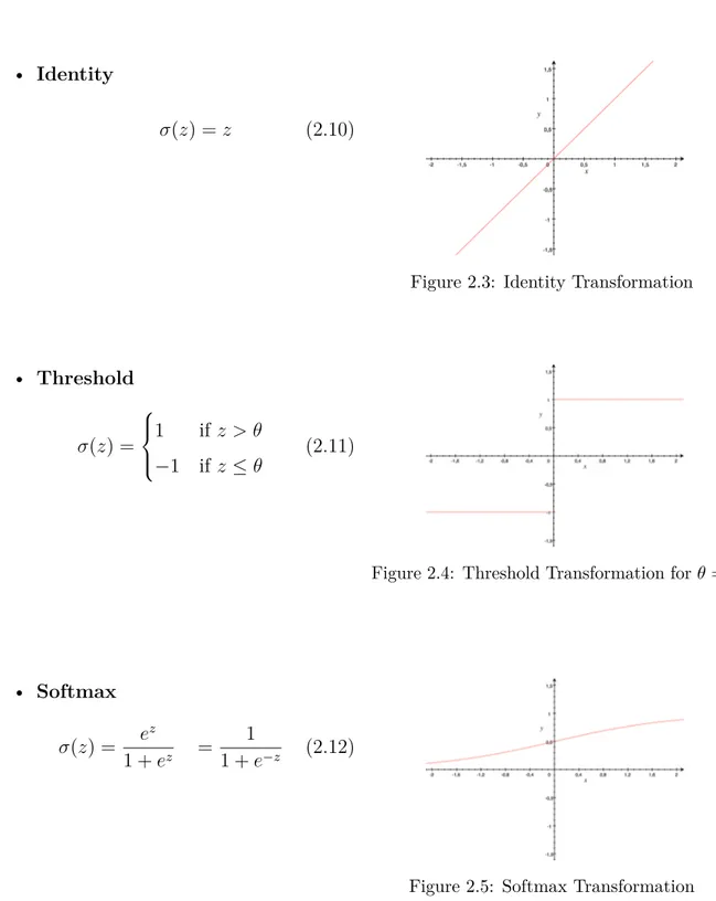
• Identity
‡(z) = z (2.10)
Figure 2.3: Identity Transformation
• Threshold ‡(z) = Y _ ] _ [ 1 if z > ◊ ≠1 if z Æ ◊ (2.11)
Figure 2.4: Threshold Transformation for ◊ = 0
• Softmax ‡(z) = e z 1 + ez = 1 1 + e≠z (2.12)
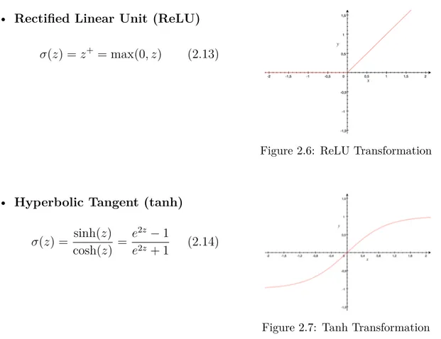
• Rectified Linear Unit (ReLU)
‡(z) = z+= max(0, z) (2.13)
Figure 2.6: ReLU Transformation
• Hyperbolic Tangent (tanh)
‡(z) = sinh(z)
cosh(z) =
e2z ≠ 1
e2z + 1 (2.14)
Figure 2.7: Tanh Transformation
Activation functions generally limit the range of values that a node will take, except the Identity transformation, which is rarely used as values can grow exponentially over the different layers. Softmax and Thresholds are used when the final output will be a discrete value, such as [0, 1]. The ReLU activation in particular, is very useful when values can’t be negative or for large datasets, since a node with a negative value is automatically cancelled from the equation, by taking a 0 value. But, if we don’t want to lose information in a regression, the tanh function is usually recommended.
2.2.2 Hidden Layers
Hidden layers have been mentioned a couple times until now. As one can deduce, hidden layers compose the internal structure of an ANN.
According to Alpaydın (2010), a Perceptron or an ANN that has a single layer of weights can only approximate linear functions of the input. But, several Perceptrons can be stacked to form a Multilayer Perceptron (MLP). These MLP can implement nonlinear discriminants in classification and can approximate nonlinear functions of the input, if used for regression.
Figure 2.8: MLP Structure
In the structure of a MLP such as the one shown in figure Figure 2.8, the input and output layers are not counted as hidden layers. Thats why, Figure 2.2 was referred as a single layer ANN.
The standard notation for the hidden layers will be superscript [l], l = 1, ..., L, where
L is the number of layers in the network. This notation is extended to all the parameters:
• n[l] : number of hidden units of the lth layer.
• a[l] : activated value of the hidden units of the lth layer.
• W[l] : weight matrix of the lth layer.
• b[l] : bias vector of the lth layer.
Each layer can have its own activation function.
2.2.3 Learning Rule
The learning rule is defined as the algorithm which optimizes the weights of an ANN in order to fit the desired output.
There are some different learning rules used in the literature, but before introducing them, we will need to talk about the building blocks for the optimization functions used to train the weights. Therefore, we will define both the cost and the propagation functions before moving on to the optimization algorithms.
2.2.3.1 Cost Function
Given some predictions ˆy œ IRn, and the desired output y, a loss function, L(ˆy, y) measures
the discrepancy between them. In other words, it computes the error for a single training example.
In ML there are six main loss functions which are commonly used. Different loss functions are more or less accurate for different data structures. In particular, one can distiguish discrete and continuous loss functions.
Discrete Functions
Two of the most common discrete loss functions, are categorical crossentropy and the
hinge loss:
• Categorical Cross Entropy
L(ˆy, y)CE = ≠ n ÿ i=1 yi· log ˆyi (2.15) • Hinge Loss
L(ˆy, y)HL = max(0, 1 ≠ ˆy · y) (2.16)
The categorical crossentropy is also called the log loss function and its sum corresponds to the log-likelihood function for logistic regression which is why it is commonly used for this model. The hinge loss instead is usually applied to classification problems which use algorithms such as Support Vector Machines.
Continuous Functions
For this case, the most common loss functions, are the Root Mean Square Error and the Mean Absolute Error:
• Root Mean Square Error
L(ˆy, y)RM SE = ˆ ı ı Ù1 n n ÿ i=1 (ˆyi ≠ yi) (2.17)
• Mean Absolute Error
L(ˆy, y)M AE = n
ÿ
i=1
|ˆyi≠ yi| (2.18)
While these work well for continuous outputs, they wouldn’t have been optimal for dichomotic answers treated in logistic regression for example, where these metrics will lead to a non-convex optimization problem, i.e. it results in an optimization problem with multiple local optima. Thus, in order to find the global optima, we need to correctly define this measure.
The cost function is the average of the loss function of the entire training set. It optimizes, W and b to minimize the overall cost, J(W , b).
2.2.3.2 Propagation Function
Given the parameters W , b and the corresponding cost function, J(W , b), we can find the local minimum using an optimization algorithm. If the defined cost function is convex, it will guarantee that this local optima is also the global optima.
In ANN, this optimization is implemented in two directions, what we call forward and backward propagation.
Forward Propagation
Forward propagation is just the sequential computation of the nodes. Therefore, the
propagation function is defined as the computation of the input of a neuron, given
the weights and the values of all the nodes in the previous layer that are connected to it, and the application of the corresponding activation function. The most general forward propagation equation is:
a[l] = g(W[l≠1]Tx[l≠1]+ b[l≠1]) (2.19)
Backward Propagation
Backward propagation is the reverse process of updating the weights from the end to the beggining. In order to do so, it computes the error of the values obtained through the forward propagation phase, which must have been done before. This computation will depend on the chosen optimization algorithm, which we present in the following section.
2.2.3.3 Optimization Algorithms
We present and build the backpropagation functions of three main optimization alogrithms: gradient descent, RMSprop and Adam optimization.
Gradient Descent
Gradient Descent, is an optimization method which iteratively optimizes differentiable cost function. It is based on the traditional optimization of functions: if we want to find
W and b that minimize a particular cost function, J(W , b), we can find this minimum
value by taking the partial derivatives equal to 0, JÕ(W , b) = 0
Thus, in Gradient Descent, the weights and the bias are updated according to the following functions:
W : = W ≠ – · ˆJ(W , b)
ˆW (2.20)
b: = b ≠ – · ˆJ(W , b)
ˆb (2.21)
where – indicates the learning rate, which determines the magnitude of change to be made in the parameter. It is generally taken between 0.0 and 1.0, but mostly – Æ 0.2. We can get an intuition of why we are interested in small learning rates from the follwing graph:
Figure 2.9: Gradient Descent Learning Rates
The problem with a fixed learning rate is that it can be very slow to converge if it isn’t properly tuned. Therefore, an adaptative learning rate can be introduced either manually or through other optimization methods which speed up this convergence.
RMSprop
RMSprop, which stands for Root Mean Square Propagation, is an optimization algorithm which speeds up the convergence of the values, by denoising some unnecessary oscilations. This is very important in ML applications, since we are not talking about an IR2 dimensional
space, as shown in Figure 2.9 but a very high dimensional space instead. Thus, if steps are taken in the wrong direction it can be very hard to eventually reach the optimal value.
average of the squares of the derivatives. At each iteration, i, Sˆwi and Sˆbi are computed as follows: Sˆwi = —2Sˆwi≠1 + (1 ≠ —2) A ˆJ(W , b) ˆW B2 (2.22) Sˆbi = —2Sˆbi≠1 + (1 ≠ —2) A ˆJ(W , b) ˆb B2 (2.23)
Sˆw0 = 0 and Sˆb0 = 0. The parameters W and b are updated according to the following
equations: W : = W ≠ – · Ô 1 Sˆwi+ Á · ˆJ(W , b) ˆW (2.24) b: = b ≠ – · Ô 1 Sˆbi + Á · ˆJ(W , b) ˆb (2.25)
The main advantage is that —2 can be fixed to 0.999 and tuning – becomes less
important, since the learning rate is indirectly decayed at each iteration. A very small value Á = 10≠8 is usually added in order to avoid zero divisions.
Adam Optimization
Finally, the Adam optimization algorithm is an extension to stochastic gradient descent, which combines momentum and RMSprop and puts them together. This algorithm has gained a lot of popularity in DL.
Additionally to the terms presented in RMSprop, the Adam optimizer introduces the momentum exponentially weighted averages, Vˆwi and Vˆbi at each iteration. The full
formulation is the following:
Given, Vˆw0 = 0, Vˆb0 = 0, Sˆw0 = 0 and Sˆb0 = 0. Vˆwi = —1Sˆwi≠1 + (1 ≠ —1) ˆJ(W , b) ˆW (2.26) Vˆbi = —1Sˆbi≠1 + (1 ≠ —1) ˆJ(W , b) ˆb (2.27)
Sˆwi = —2Sˆwi≠1 + (1 ≠ —2) A ˆJ(W , b) ˆW B2 (2.28) Sˆbi = —2Sˆbi≠1 + (1 ≠ —2) A ˆJ(W , b) ˆb B2 (2.29) W : = W ≠ – · Ô Vˆwi Sˆwi + Á (2.30) b: = b ≠ – · Ô Vˆbi Sˆbi + Á (2.31)
As in RMSprop, —2 = 0.999 and —1 can be fixed to 0.9. Again, the initial choice of –
has a lower impact on the full learning process.
2.3 Variants of Artificial Neural Networks
Now that we have seen all the building blocks of ANN, we will see that several variants of ANN can be defined according to their different arquitechtures. In particular, the three main variants used for different RS will be presented: Convolutional Neural Networks,
Recurrent Neural Networks and Autoencoders.
All of these architectures are built over several hidden layers. Hence, we are talking about deep learning algorithms.
2.3.1 Convolutional Neural Networks
Convolutional Neural Networks (CNN) are deep feed-forward ANN which are generally used for image processing. Their basic structure is the same of a regular MLP: an input layer, multiple hidden layers and an output layer. The difference falls on the architecture of the hidden layers, which include:
• Convolutional layers take all the input nodes and compute a single output instead of computing an output for each node. Mathematically, the convolution corresponds to cross-correlation. The convolution emulates the activation function, but in this case it has the advantage that is reduces the number of free parameters. This is specially relevant for images, where every pixel correspond to three diferent input values in an RGB setting.
Convolutions can be valid or same. The first reduce the dimensionality while the latter, pad the resulting output in order to keep the original dimension. Strides can also be added to convolutions in order to reduce even more the dimensions, by "jumping" part of the combinable clusters.
• Pooling layers reduce the dimensions of the original image by clustering several pixels and combining them into one node. There are two main clustering techniques than can be applied: max pooling, which takes the highes value from each cluster; or
average pooling, which computes the average of all the pixels in a cluster.
• Fully-connected layers correspond to the traditional layers where every node from one layer is connected to all the neurons in the following one.
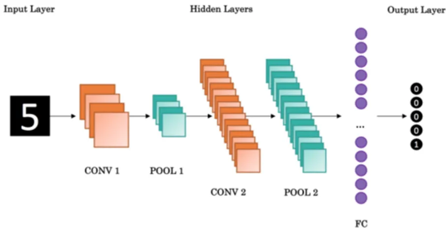
One setting in particular, known as the LeNet-5, became very famous for optical character recognition. Its structure can be depicted as follows:
Figure 2.10: LeNet-5 5-layer CNN for Optical Character Recognition
CNN can also be used for image classification, and for object detection, where several objects can be detected inside a single image. Videos and movies can be seen as a sequence of images, thus, CNN are used in combination with RNN to make video and movie recommendations.
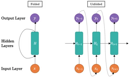
2.3.2 Recurrent Neural Networks
Recurrent Neural Networks (RNN) are deep ANN, that, unlinke feed-forward networks, retain previous information to process sequences. In order to do so they can have a single output at the end or several sequential outputs in intermediate layers, which, in its turn, are feed to the inputs of the next layer.