New techniques of molecular modelling and structural chemistry for the development of bioactive compounds

(1)

UNIVERSITY OF SALERNO

DEPARTMENT OF PHARMACY

PhD course in Scienza e Tecnologie per l’Industria Chimica, Farmaceutica e Alimentare

XI course NS (XXV) 2009-2012

New techniques of molecular modelling and structural chemistry

for the development of bioactive compounds

Tutor PhD student

Prof. Giuseppe Bifulco Gianluigi Lauro

Coordinators

Prof.Nunziatina De Tommasi

(2)

Preface

My PhD three years course in Pharmaceutical Sciences at the Department of Pharmaceutical and Biomedical Sciences of Salerno University was started in 2010 under the supervision of Prof. Giuseppe Bifulco.

My research activity was mainly focused on studies of ligand-receptor interactions and structural characterization by computational techniques in order to identify new antitumor molecules potentially utilizable in therapy.

In particular, I was mainly interested into the development of a new computational technique named Inverse Virtual Screening. The application of this approach led to the identification of the targets of interaction of several natural compounds.

Furthermore, to improve my knowledge on computational chemistry, I moved to the The University Pompeu Fabra-PRBB (Parc de Recerca Biomèdica de Barcelona) in 2012 (mid-May until end of October 2012) under the supervision of Dr. Gianni De Fabritiis.

During this period in his laboratory, my research work has included learning High-throughput Molecular Dynamics simulations, taking the advantage of his expertise in the field of molecular simulation applied to relevant systems in a drug design perspective, and his unique hardware and software infrastructure (GPU grid–ACEMD software).

In addition to PhD course activities, I was involved in several other projects, mainly regarding the characterization of ligand-targets interactions of ligands on receptor targets (PXR, PPAR-γ, HSP70 1A), in order to elucidate the molecular basis of their activity.

(3)

List of publications related to the scientific activity performed during the three years PhD course in Pharmaceutical Sciences:

1 Dal Piaz, F.; Cotugno, R.; Lepore, L.; Vassallo, A.; Malafronte, N.; Lauro, G.; Bifulco, G.; Belisario, M. A.; De Tommasi, N. Chemical Proteomics Reveals HSP70 1A as a Target for the Anticancer Diterpene Oridonin. J.Proteomics, submitted

2 Festa, C.; Lauro, G.; De Marino, S.; D’Auria, M. V.; Monti, M. C.; Casapullo, A.; D’Amore, C.; Renga, B.; Mencarelli, A.; Petek, S.; Bifulco, G.; Fiorucci, S.; Zampella, A. Plakilactones from the marine sponge Plakinastrella mamillaris. Discovery of a new class of marine ligands of peroxisome proliferator-activated receptor γ. J. Med. Chem. 2012, 55, 8303-8317.

3 Sepe, V.; Ummarino, R.; D'Auria, M. V.; Lauro, G.; Bifulco, G.; D'Amore, C.; Renga, B.; Fiorucci, S.; Zampella, A. Modification in the side chain of solomonsterol A: discovery of cholestan disulfate as a potent pregnane-X-receptor agonist. Org. Biomol. Chem. 2012, 10, 6350-6362.

4 Lauro, G.; Masullo, M.; Piacente, S.; Riccio, R.; Bifulco, G. Inverse Virtual Screening allows the discovery of the biological activity of natural compounds.

Bioorg. Med. Chem. 2012, 20, 3596-3602.

5 Cheruku, P.; Plaza, A.; Lauro, G.; Keffer, J.; Lloyd, J. R.; Bifulco, G.; Bewley, C. A. Discovery and synthesis of namalide reveals a new anabaenopeptin scaffold and peptidase inhibitor. J. Med. Chem. 2012, 55, 735-742.

(4)

6 Lauro, G.; Romano, A.; Riccio, R.; Bifulco, G. Inverse virtual screening of antitumor targets: pilot study on a small database of natural bioactive compounds.

(5)

Abstract

Computational chemistry represents today a valid and fast tool for the research of new compounds with potential biological activity. The analysis of ligand-macromolecule interactions and the evaluation of possible “binding modes” have a crucial role for the design and the development of new and more powerful drugs. In

silico Virtual Screening campaigns of large libraries compounds (fragments or

drug-like) on a specific target allow the selection of promising compounds, leading the identification of new scaffolds. The accurate analysis and the comparison of different bioactive compounds clarify the molecular basis of their interaction and the construction of pharmacoforic models.

In parallel, another crucial aspect of pharmacological research is the identification of targets of interaction of bioactive molecules, and this is particularly true for compounds from natural sources. In fact, a wide range of drug tests on a large number of biological targets can represent a useful approach for the study of natural products, but often one of the main problems is their limited availability.

Starting from these assumptions, a new computational method named Inverse Virtual Screening is described in details in this thesis. The different works based on this approach were performed considering panels of targets involved in the cancer events, determining the identification of the specific antitumor activity of the natural compounds investigated.

Inverse Virtual Screening studies were performed by means of molecular docking experiments on different natural compounds, organized in small libraries or as single compounds. Firstly, a mathematical method for the exclusion of false positive and false negative results was proposed applying a normalization of the predicted binding energies (expressed in kcal/mol) obtained from the docking calculations (paragraph 2.2). Then this approach was applied on a library of 10

(10)

II

compounds extracted from natural sources (paragraph 2.3), obtaining a good validation through in vitro biological tests. Afterwards, another study was performed on the cyclopeptide namalide. Its biological inhibitory activity and selectivity on Carboxipeptidase A target was in accordance with Inverse Virtual Screening results (paragraph 2.4).

Virtual Screening topic was also inspected analyzing the efficacy of Molecular Dynamics-based methods for the accurate calculations of the binding affinities. This work was conducted on a library of 1588 compounds (44 ligands + 1544 decoys) extracted from the DUD database on trypsin target, using the Linear Interaction Energy (LIE) method by means of extensive Molecular Dynamics simulations. Four different LIE results obtained combining different scaling factors were compared with docking results, evaluating and comparing ROC and enrichment curves for each of the considered methods. Poor results were obtained with LIE, and further analysis with MM-GBSA and MM-PBSA approaches are under investigation.

Moreover, in silico screenings were performed for the detailed study of natural compounds whose activities are known a priori. With this procedure, several binding modes were reported for a library of compounds on PXR target, whose activity or inactivity were rationalized comparing their binding poses with that of Solomonsterol A, used as a reference compound on this receptor. The presence/absence of biological activity of another library of compounds extracted from the marine sponge Plakinastrella Mamillaris on PPAR-γ and for the diterpene oridonin on HSP70 1A are described at a molecular level respectively in paragraphs 4.2 and 4.3 with molecular docking and Molecular Dynamics simulations.

The putative binding modes for the reported molecules was described offering a complete rationalization of docking results, evaluating how ligand target specific

(11)

III

interactions (e.g. hydrophobic, hydrophilic, electrostatic contacts) can influence their biological activity.

(12)

1

(13)

2

-CHAPTER 1-

Computational chemistry and drug discovery

(14)

3

1.1 Drug discovery process and computational chemistry

Drug discovery is an expensive process including the identification and validation of a drug target (typically a protein), determination of 3-D structure of that target, discovery of a lead compound that binds to the target and development of the lead into a drug candidate.

Computational chemistry represents today the preferential tool for predicting the putative binding modes and affinities of chemical compounds bound to a target. The difficulties and economic cost of the experimental methods explain the fast development of computational chemistry during the past years. The early development of computational chemistry was dependent on the developments in computational power and techniques. Computing power became widely available in the 1960s and a great number of new numerical models, or algorithms, were constantly produced worldwide. As computer power increased, the mathematical equations were refined in order to model real life more accurately.

Effective use of computational chemistry shortens the development cycle for new drugs and provides pharmaceutical companies a competitive advantage with faster time-to-discovery and reduced costs. Numerous examples of drugs have been discovered and optimized with contributions from computational chemists.1 The primary goal of computational chemistry in drug discovery is to develop quantitative models that are able to predict activities of compounds quickly and accurately. Computer hardware and software is used to simulate a chemical process or to compute a chemical property. While it is now recognised that high-throughput methods are amply capable of producing greater volumes of data, they do not always increase the productivity and timeliness of a research effort. The problem in laboratories today is not one of acquiring data at each stage of drug discovery, but rather of extracting the useful information from the wealth that is available.

(15)

4

Fortunately, computational power and data-mining techniques are also advancing in step with demand.

Computational methods provide guidance but are by no means able to make perfect predictions. Molecular libraries are screened, and the resulting leads are optimized in a cycle that features design, synthesis and assaying of numerous analogs, and animal studies. Crystal structure determination for complexes of some analogs with the biomolecular target is often possible, which enables “structure-based drug design” (SBDD)2 and the efficient optimization of leads. SBDD is based on the knowledge of the 3-dimensional structure of the protein and, preferably co-complexed with a ligand as an identifier of the binding site are exploited for the design and the optimization of lead compounds.3,4,5

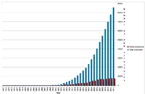
Figure 1.1 Number of yearly and total PDB structures available on PDB database from 1972

(16)

5

As shown in Figure 1.1, a constantly growing number of protein structures have become available each year since 1976. As of February 2013, almost 85000 protein structures have been deposited at the Protein Data Bank (PDB),6,7 and this strongly demonstrates that structure-based drug design will continue to play a significant role in the field of drug design and discovery.

Briefly, in the SBDD method, starting from the structure of a protein or a nucleic acid (X-ray crystallography, NMR or homology modelling), compounds or fragments of compounds from a database are positioned into a selected region of the structure. These compounds are scored and ranked, and the best compounds are tested with biochemical assays. In a next phase, from the results obtained it is possible to reveal parts of the compound that can be optimized to increase potency. This processes can be re-iterated, and then the optimazed compounds usually show marked improvement in binding and/or specificity for the target.

The recognition of the binding site or the active site residues in the target structure is of high importance in SBDD. Basically, it is a small region, a pocket or bumps, where ligand molecules can best fit or bind to activate the receptor and/or target and produce the desirable effect. Since the proteins are capable of undergoing conformational changes, recognizing the accurate binding site residues is difficult;8 but still there are just a few computational programs, such as Ligsitecsc,9 Qsite finder10 and CASTp,11 that can capably spot out the binding site residues. For example, Qsite finder locates and clusters the favorable binding sites using the interaction energy and Van der Waal’s probes, whereas CASTp employs functionally annotated residues for mapping the surface pockets.

In this context, starting from a defined target structure, one of the most popular approaches used is the Virtual Screening (VS) from millions of potential compounds. VS computationally screens large chemical libraries to search for compounds that possess complementarities toward the targets.12,13 The screening of

(17)

6

compounds in VS is carried out using docking calculations where the compounds are filtered mainly considering their binding energies against the target.13,14 Because these types of screening techniques are mainly data driven, data accessibility remains highly significant.

Another approach often used is the “ligand-based drug design”, very useful in the absence of an experimental 3D structure.15,16 Due to the lack of an experimental structure, the known ligand molecules that bind to the drug target are studied and compared to understand their structural and physico-chemical properties that correlate with the desired pharmacological activity.17 Ligand-based methods may also include natural products or substrate analogues that interact with the target molecule yielding the desired pharmacological effect.18,19 Here, if sufficient number of reported active compounds (10-40) with diverse activity values are there, one can build a 3D pharmacophore model of these set of compounds by overlapping all of them and finding the common feature among them.

SBDD and LBDD approaches can be used for the de-novo design, a process of creating or building new lead compounds from scratch - the former method being more prevalent than the latter. This process complements VS in hit discovery. The main principle of de novo design is to construct the small-molecule chemical structures that best fit the target space.20 In receptor-based de novo design high-quality protein structures and their respective binding sites are essential because the hits are designed based on the target structures by placing small fragments in the key interaction sites of the proteins. Receptor-based design can be carried out by two means: linking and growing techniques.

(18)

7

(19)

8

In the linking process different small fragments from the libraries are added simultaneously to different active site residues of the target.21 Thus, the small fragments positioned at the binding site link to each other and form a final single compound. This approach is widely preferred because the fragment design strategy is insightful in that most biological targets encompass discrete binding sites for each piece of a ligand.

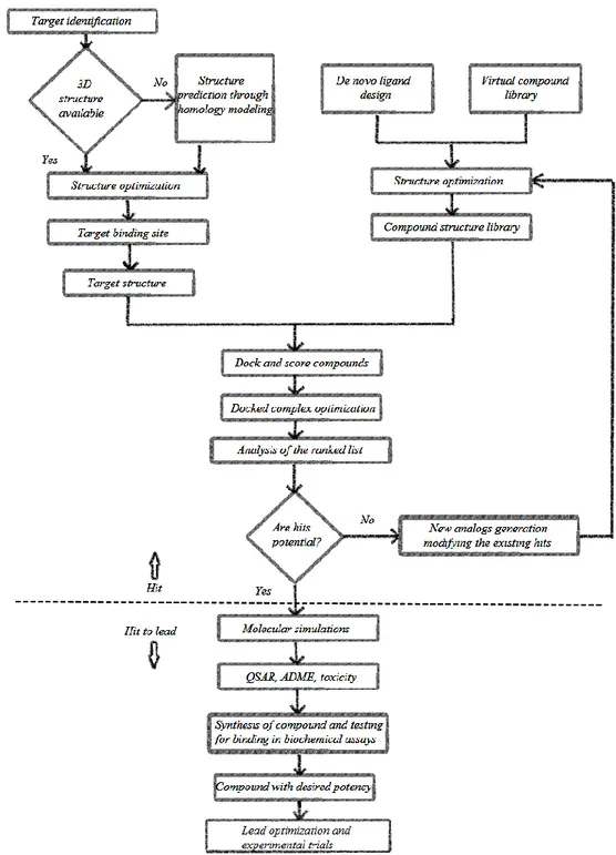
Whereas, in the growing technique a single small fragment is placed in the active site of the target and this fragment grows well complementarily against the receptor-binding site – thereby resulting in a library of chemical compounds that are more specific to the target. The process flow for the “hit identification” phase and “hit-to-lead” phase is represented in Figure 1.2.

(20)

9

1.2 Methodologies employed

A summary of the main methodologies used to realize the project is briefly presented in the next paragraphs.

1.2.1 Molecular Docking

One of the more current and fast computational techniques used in the field of the medicinal chemistry is represented by the molecular docking. With this computational tool, based on the protein structures, thousands of possible poses of association are tried and evaluated. Many different docking software have been developed, i.e. GOLD,22 DOCK,23 FlexX,24 Autodock 3,25 Autodock 4,26 Autodock 4.2,27 Autodock-Vina,28 Glide.29

When only the structure of a target and its active or binding site is available, high-throughput docking is primarily used as a hit identification tool. The determination of the binding mode and affinity between the constituent molecules in molecular recognition is crucial to understanding the interaction mechanisms and to designing therapeutic interventions. However, similar calculations are often also used later on during lead optimization, when modifications to known active structures can quickly be tested in computer models before compound synthesis.

Thus, if a particular target structure is known, one can dock a library of different chemical compounds into the same binding site, obtain a scoring value for each pose, and in this way virtually screen for affinity towards the target. High throughput virtual screening (HTVS), where the library may consist of up to 1012 (virtual) compounds, is a procedure commonly employed by pharmaceutical companies when starting a new lead discovery process. When desiring more detailed information about a potential ligand–protein complex than can be provided by HTVS, the assumption of the protein being a rigid structure becomes harder to

(21)

10

justify. It is well known that most, if not all, proteins continuously undergo conformational changes when exerting their functions in vivo.30 Specifically, when an agonist binds to a receptor, it is clear that significant conformational changes must take place. In light of this, some attempts have been made to take protein flexibility into account during docking. However, scoring all possible conformational changes is prohibitively expensive in computer time. Docking procedures which permit conformational change, or flexible docking procedures, must intelligently select small subset of possible conformational changes for consideration.

In general, there are two aims of docking studies: accurate structural modelling and correct prediction of activity.

Basically, a protein-ligand docking program consists of two essential components, sampling and scoring.

1.2.1.1 Sampling

Sampling refers to the generation of putative ligand binding orientations/conformations near a binding site of a protein and can be further divided into two aspects, ligand sampling and protein flexibility.

Ligand sampling is the most basic element in protein-ligand docking. Given a protein target, the sampling algorithm generates putative ligand orientations/conformations (i.e., poses) around the chosen binding site of the protein.

Treatment of ligand flexibility can be divided into three basic categories:31 systematic methods (incremental construction, conformational search, databases); random or stochastic methods (Monte Carlo, genetic algorithms, tabu search); and simulation methods (Molecular Dynamics, energy minimization).

(22)

11

Systematic search algorithms generate all possible ligand binding conformations by exploring all degrees of freedom of the ligand.

The most straightforward systematic algorithms are exhaustive search methods, in which flexible-ligand docking is performed by systematically rotating all possible rotatable bonds of the ligand at a given interval. Despite its sampling completeness for ligand conformations, the number of the combinations can be huge with the increase of the rotatable bonds.

In stochastic algorithms, ligand binding orientations and conformations are sampled by making random changes to either a single ligand or a population of ligands at each step in both the conformational space and the translational/rotational space of the ligand, respectively. A newly obtained ligand is evaluated on the basis of a pre-defined probability function. Two popular random approaches are Monte Carlo and genetic algorithms.

For what concerns simulation methods, Molecular Dynamics and energy minimization are the most popular simulation approaches. Molecular Dynamics simulations are often unable to cross high-energy barriers within feasible simulation time periods, and therefore might only accommodate ligands in local minima of the energy surface.

Therefore, an attempt is often made to simulate different parts of a protein– ligand system at different temperatures.32

Another strategy for addressing the local minima problem is to perform Molecular Dynamics calculations from different ligand positions. In contrast to Molecular Dynamics, energy minimization methods are rarely used as stand-alone search techniques, as only local energy minima can be reached, but often complement other search methods, including Monte Carlo.

For example, DOCK performs a minimization step after each fragment addition, followed by a final minimization before scoring.

(23)

12

Protein flexibility starts from the assumption that ligand binding commonly induces protein conformational changes, which range from local rearrangements of side-chains to large domain motions. Methods to account for protein flexibility can be grouped into three categories: soft docking, side-chain flexibility, and protein ensemble docking.

Soft docking is the simplest method which considers protein flexibility implicitly. It works by allowing for a small degree of overlap between the ligand and the protein through softening the interatomic van der Waals interactions in docking calculations.

In side-chain flexibility method backbones are kept fixed and side-chain conformations are sampled.

The third type of methods account for protein flexibility by firstly using rigid-body docking to place the ligand into the binding site and then relaxing the protein backbone and side-chain atoms nearby.

Specifically, the initial rigid-body docking allows for atomic clashes between the protein and the placed ligand orientations/conformations in order to consider the protein conformational changes. Then, the formed complexes are relaxed or minimized by Monte Carlo (MC), Molecular Dynamic simulations, or other methods.

In general, the most widely-used type of methods for incorporating protein flexibility utilizes an ensemble of protein structures to represent different possible conformational changes.

The ensemble docking algorithm is not used for generating new protein structures, but instead for selecting the induced-fit structure from a given protein ensemble. Following a similar procedure, Abagyan and colleagues expanded Huang and Zou’s algorithm to create ICM’s ensemble docking algorithm, referred to as four-dimensional (4D) docking.33

(24)

13

1.2.1.2 Scoring

Scoring is the prediction of the binding tightness for individual ligand orientations/conformations with a physical or empirical energy function. The top orientation/conformation, namely the one with the lowest energy score, is typically predicted as the binding mode. The scoring function is a key element of a protein-ligand docking algorithm, because it directly determines the accuracy of the algorithm.34,35,36,37 Speed and accuracy are the two important aspects of a scoring function and an ideal scoring function would be both computationally efficient and reliable. Scoring functions have been developed can be grouped into three basic categories:

 force field

 empirical

 knowledge-based scoring functions.

Force field (FF) scoring functions25,38,39 are based on decomposition of the ligand binding energy into individual interaction terms such as van der Waals (VDW) energies, electrostatic energies, bond stretching/bending/torsional energies, etc., using a set of derived force-field parameters such as AMBER40 or CHARMM41,42 force fields. In general, the enthalpic contributions are essentially given by the electrostatic and van der Waals terms, and also considering taking into account the hydrogen bond formation between drug and biological target.

The van der Waals potential energy is often modeled by the Lennard-Jones 12-6 function (Equation 1.1) Equation 1.1

(25)

14

where ε is the well depth of the potential and σ is the collision diameter of the respective atoms i and j. The exp(12) is responsible for small-distance repulsion, whereas the exp(6) is related to an attractive term which approaches zero as the distance between two atoms increases (Figure 1.3).

Figure 1.3 Graphical representation of the Lennard-Jones 12-6 function

This Lennard-Jones 12-6 function is also used to describe the hydrogen bond in macromolecule-ligand complex, but is less smooth and angle dependent if compared to the van Der Waals function.

The electrostatic potential energy is represented as the summation of Coulombic interactions, as described in Equation 1.2:

Equation 1.2

Where N is the number of atoms in molecules A and B, respectively, and q is the charge on each atom. The functional form of the internal ligand energy is typically very similar to the ligand-protein interaction energy, and also includes van der Waals contributions and/or electrostatic terms.

(26)

15

One of the major challenges in FF scoring functions is how to account for the solvent effect. The simplest method is to use a distance-dependent dielectric constant (rij) such as the force field scoring function in DOCK39 (Equation 1.3)

Equation 1.3

where rij stands for the distance between protein atom i and ligand atom j, Aij

and Bij are the VDW parameters, and qi and qj are the atomic charges. ε(rij) is

usually set to 4rij, reflecting the screening effect of water on electrostatic

interactions. The most rigorous FF methods are to treat water molecules explicitly. However, these methods, together with their simplified approaches such as LIEPROFEC, and OWFEG are computationally expensive.43 To reduce the computational expense, accelerated methods have been developed while preserving the reasonable accuracy by treating water as a continuum dielectric medium. The Poisson-Boltzmann/surface area (PB/SA) models44,45,46 and the generalized-Born/surface area (GB/SA) models47,48,49 are typical examples of such implicit solvent models.

In addition to the challenge on solvent effect, how to accurately account for entropic effect is an even more severe challenge for FF scoring functions. Moreover, whether the free energy of ligand binding can be decomposed into a linear combination of individual interaction terms without calculating the partition function (“ensemble average”) also remains in question, referred to as the nonadditive problem.

The second type of scoring function (empirical scoring functions) works on the sum of a set of weighted empirical energy terms such as VDW energy, electrostatic

(27)

16

energy, hydrogen bonding energy, desolvation term, entropy term, hydrophobicity term, etc.(Equation 1.4):

Equation 1.4

where {ΔGi} represent individual empirical energy terms, and the corresponding coefficients {Wi} are determined by reproducing the binding affinity

data of a training set of protein-ligand complexes with known three-dimensional structures, using least squares fitting. GlideScore50,51, PLP52, SYBYL/F-Score,24 LigScore,53 LUDI,54 SCORE,55 X-Score,56 ChemScore,57 MedusaScore,58 AIScore,59 and SFCscore60 are examples of empirical scoring functions.

In knowledge-based scoring functions protein-ligand complexes are modeled using relatively simple atomic interaction-pair potentials. In essence, it is designed to reproduce experimental structures rather than binding energies. A number of atom-type interactions are defined depending on their molecular environment. Compared to the force field and empirical scoring functions, the knowledge-based scoring functions offer a good balance between accuracy and speed. Namely, because the potentials are extracted from a large number of structures rather than attempting to reproduce the known affinities by fitting, the knowledge-based scoring functions are relatively robust and general. Their pairwise characteristic also enables the scoring process to be as fast as empirical scoring functions.

A technique to improve the performances of scoring functions is clustering-based scoring methods, which incorporate the entropic effects by dividing generated ligand binding modes into different clusters.61,62,63 The entropic contribution in each cluster is measured by the configurational space covered by the ligand poses or the number of the ligand poses in the cluster.

(28)

17

One restriction in clustering-based scoring methods is that its performance depends on the ligand sampling protocol that is used, i.e., it is docking program-dependent. These methods in combination with ligand conformational sampling using AutoDock have significantly improved binding mode prediction.

1.2.1.3 Autodock: An Overview

AutoDock currently represents one of the most cited docking softwares,64 especially in a virtual screening of a compound libraries.65 For the purposes of this project the software AutoDock 3.0.5,25 4,26 4.2,27 and Autodock-Vina28 have been used.

Basically, the differences between them are related to the speed, macromolecule sidechains flexibility, optimization of the free-energy scoring function based on a linear regression analysis, AMBER force field, larger set of diverse protein-ligand complexes with known inhibition constants; moreover the Lamarckian Genetic Algorithm (LGA) is a big improvement on the Genetic Algorithm, and both genetic methods are much more efficient and robust than SA in the new version of the software.

In AutoDock there are different available search methods, but the Lamarckian Genetic Algorithm (LGA) has been selected for the aim of this study, because it has demonstrated to give the best results compared to the other algorithms.25

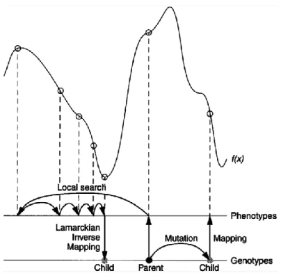
The vast majority of genetic algorithms mimics the characteristics of Darwinian evolution and applies Mendelian genetics. This is briefly illustrated in Figure 1.4.

This is called the Lamarckian genetic algorithm (LGA), and is an allusion to Jean Batiste de Lamarck’s (discredited) assertion that phenotypic characteristics acquired during an individual’s lifetime can become heritable traits.66

(29)

18

Figure 1.4 This figure illustrates genotypic and phenotypic search, and contrasts Darwinian and

Lamarckian search.67 The space of the genotypes is represented by the lower horizontal line, and the space of the phenotypes is represented by the upper horizontal line. Genotypes are mapped to phenotypes by a developmental mapping function. The fitness function is f(x). The result of applying the genotypic mutation operator to the parent’s genotype is shown on the right-hand side of the diagram, and has the corresponding phenotype shown. Local search is shown on the left-hand side. It is normally performed in phenotypic space and employs information about the fitness landscape. Sufficient iterations of the local search arrive at a local minimum, and an inverse mapping function is used to convert from its phenotype to its corresponding genotype. In the case of molecular docking, however, local search is performed by continuously converting from the genotype to the phenotype, so inverse mapping is not required. The genotype of the parent is replaced by the resulting genotype, however, in accordance with Lamarckian principles.

The most important issues arising in hybrids (LGA) of Genetic Algorithm (GA) and the Local Search (LS) revolve around the developmental mapping, which transforms genotypic representations into phenotypic ones.

The genotypic space is defined in terms of the genetic operators mutation and crossover in our experiments by which parents of one generation are perturbed to form their children. The phenotypic space is defined directly by the problem,

(30)

19

namely, the energy function being optimized. The local search operator is a useful extension of GA global optimization when there are local ‘‘smooth-ness’’ characteristics (continuity, correlation, etc.) of the fitness function that local search can exploit. In hybrid GA + LS optimizations, the result of the LS is always used to update the fitness associated with an individual in the GA selection algorithm. If, and only if, the developmental mapping function is invertible, will the Lamarckian option converting the phenotypic result of LS back into its corresponding genotype become possible. The fitness or energy is usually calculated from the ligand’s coordinates, which together form its phenotype. The developmental mapping simply transforms a molecule’s genotypic state variables into the corresponding set of atomic coordinates. A novel feature of this application of hybrid global-local optimization is that the Solis and Wets LS operator searches through the genotypic space rather than the more typical phenotypic space. This means that the developmental mapping does not need to be inverted. Nonetheless, this molecular variation of the genetic algorithm still qualifies as Lamarckian, because any ‘‘environmental adaptations’’ of the ligand acquired during the local search will be inherited by its offspring. At each generation, it is possible to let a user defined fraction of the population undergo such a local search. The local search frequencies of just 0.06 have found improved efficiency of docking, although a frequency of 1.00 is not significantly more efficient.67 Both the canonical and a slightly modified version of the Solis and Wets method have been implemented. In canonical Solis and Wets, the same step size would be used for every gene, but we have improved the local search efficiency by allowing the step size to be different for each type of gene: a change of 1 Å in a translation gene could be much more significant than a change of 1° in a rotational or torsional gene. In the Lamarckian genetic algorithm, genotypic mutation plays a somewhat different role than it does in traditional genetic algorithms. Traditionally, mutation plays the role of a local search operator,

(31)

20

allowing small, refining moves that are not efficiently made by crossover and selection alone. With the explicit local search operator, however, this role becomes unnecessary, and is needed only for its role in replacing alleles that might have disappeared through selection. In LGA, mutation can take on a more exploratory role.

The LGA yields a maximum number of 256 potential bioactive conformations: run, whose number can be increased performing more docking calculations. Each conformational solution is the result of a selection. The GA, starting from the input geometry, gives rise to a group of n conformations or individuals (whose number can be set up) defining for them translational, rotational and torsional variables. By the scoring function, each individual is labeled by the total interaction energy (fitness).

Random pairs of individuals are mated using a process of crossover, in which new individuals inherit geometrical features from their parents leading to new generation of individuals. In addition, some offspring undergo random mutation, in which the translational, rotational and torsional variables are mutated randomly. Selection of the offspring of the current generation occurs based on the individual’s fitness: thus the better solutions go on into the next generations, whereas conformations with a low fitness are discarded. This cycle of crossover, mutation to lead new generation is repeated until the better bioactive conformation (run) is given.

The LS performs an energy minimization of the current found conformation. In each generation a fraction of conformations population undergoes the geometry optimization, based on the local search frequency. Rapid energy evaluation is achieved by precalculating atomic affinity potentials (grid maps) for each atom type in the substrate molecule by grid method.68

(32)

21

These maps are calculated by AutoGrid. In this procedure the protein is embedded in a three dimensional grid and a probe atom is placed at each grid point (Figure 1.5). The energy of interaction of this single atom with the protein is assigned to the grid point.

An affinity grid is calculated for each type of atom in the substrate, typically carbon, oxygen, nitrogen and hydrogen, as well as a grid of electrostatic potential, either using a point charge of +1 as the probe, or using a Poisson-Boltzmann finite difference method, such as DELPHI.69 The energetic of a particular substrate configuration is then found by tri-linear interpolation of affinity values of the eight grid points surrounding each of the atoms in the substrate.

The electrostatic interaction is evaluated similarly, by interpolating the values of the electrostatic potential and multiplying by the charge on the atom (the electrostatic term is evaluated separately to allow finer control of the substrate atomic charges).

The time to perform an energy calculation using the grids is proportional only to the number of atoms in the substrate, and is independent of the number of atoms in the protein. An estimated free energy of binding is used to evaluate the docked ligand conformations. This scoring function, based of force field AMBER,70 comprises terms above described (directional hydrogen bonding, electrostatics, Van der Waals, internal energy) and entropic contribution: desolvation and torsional entropy. The latter describes the loss of entropy upon interaction with macromolecule followed by immobilization in the active site.

The desolvation belongs the displacement of water molecules from the active site upon the binding of ligand to the macromolecular surface and the reorganization of solvent around the complex.

(33)

22 Figure 1.5 Schematic representation of the grid map.

The scoring function was implemented using the thermodynamic cycle of Wesson and Eisenberg. The function is:

Equation 1.5

(34)

23

where the five ΔG terms on the right hand side are coefficient empirically determined using a linear regression analysis from a set of protein-ligand complexes.25

For what concerns AutoDock Vina,28 this is a open-source program for drug discovery, molecular docking and virtual screening, offering multi-core capability, high performance and enhanced accuracy and ease of use. Vina uses a sophisticated gradient optimization method in its local optimization procedure.

The calculation of the gradient effectively gives the optimization algorithm a “sense of direction” from a single evaluation. In the spectrum of computational approaches to modelling receptor ligand binding molecular dynamics with explicit solvent, Molecular Dynamics and Molecular Mechanics with implicit solvent, molecular docking can be seen as making an increasing trade-off of the representational detail for computational speed.71 Among the assumptions made by these approaches is the commitment to a particular protonation state of and charge distribution in the molecules that do not change between, for example, their bound and unbound states.

Additionally, docking generally assumes much or all of the receptor rigid, the covalent lengths, and angles constant, while considering a chosen set of covalent bonds freely rotatable (referred to as active rotatable bonds here). Importantly, although Molecular Dynamics directly deals with energies (referred to as force fields in chemistry), docking is ultimately interested in reproducing chemical potentials, which determine the bound conformation preference and the free energy of binding. It is a qualitatively different concept governed not only by the minima in the energy profile but also by the shape of the profile and the temperature.72 Docking programs generally use a scoring function, which can be seen as an attempt to approximate the standard chemical potentials of the system. When the superficially physics-based terms like the 6–12 van der Waals interactions and

(35)

24

Coulomb energies are used in the scoring function, they need to be significantly empirically weighted, in part, to account for this difference between energies and free energies.72

The afore mentioned considerations should make it rather unsurprising when such superficially physics-based scoring functions do not necessarily perform better than the alternatives.

This approach was seen to the scoring function as more of “machine learning” than directly physics-based in its nature. It is ultimately justified by its performance on test problems rather than by theoretical considerations following some, possibly too strong, approximating assumptions

The general functional form of the conformation-dependent part of the scoring function AutoDock Vina is designed to work with is:

Equation 1.6

where the summation is over all of the pairs of atoms that can move relative to each other, normally excluding 1–4 interactions, i.e., atoms separated by three consecutive covalent bonds.

Here, each atom i is assigned a type ti, and a symmetric set of interaction

functions fti-tj of the interatomic distance rij should be defined.

This value can be seen as a sum of intermolecular and intramolecular contributions:

(36)

25

The optimization algorithm attempts to find the global minimum of c and other low-scoring conformations, which it then ranks.

The predicted free energy of binding is calculated from the intermolecular part of the lowest-scoring conformation, designated as 1:

Equation 1.8

where the function g can be an arbitrary strictly increasing smooth possibly nonlinear function.

In the output, other low-scoring conformations are also formally given s values, but, to preserve the ranking, using cintra of the best binding mode:

Equation 1.9

For modularity reasons, much of the program does not rely on any particular functional form of fti-tj interactions or g. Essentially, these functions are passed as a

parameter for the rest of the code.

In summary the evaluation of the speed and accuracy of Vina during flexible redocking of the 190 receptor-ligand complexes making up the AutoDock 4 training set showed approximately two orders of magnitude improvement in speed and a simultaneous significantly better accuracy of the binding mode prediction. In addition, Vina can achieve near-ideal speed-up by utilizing multiple CPU cores. However, AutodockVina does not provide very good weight of the energetic contribution derived from the hydrogen bond and electrostatic interactions, especially when the metal ions are presents.

(37)

26

1.2.2 Molecular Dynamics

One of the principal tools in the theoretical study of biological molecules is represented by Molecular Dynamics simulations (MD). This computational method calculates the time dependent behavior of a molecular system. MD simulations have provided detailed information on the fluctuations and conformational changes of proteins and nucleic acids. These methods are now routinely used to investigate the structure, dynamics and thermodynamics of biological molecules and their complexes, representing an important tool in the drug discovery process.73

Crystallographic studies demonstrate that protein flexibility plays a fundamental role in ligand binding, but they represents long and very expensive methods. As a consequence, computational techniques that can predict protein motions are needed. Unfortunately, the calculations required to describe the absurd quantum-mechanical motions and chemical reactions of large molecular systems are often too complex and computationally intensive for even the best supercomputers. Molecular Dynamics (MD) simulations, first developed in the late 1970s,74 seek to overcome this limitation by using simple approximations based on Newtonian physics to simulate atomic motions, thus reducing the computational complexity. The forces acting on each of the system atoms are then estimated from an equation like that shown in Equation 1.1075 and represented in Figure 1.6:

Equation 1.10

(38)

27

Figure 1.6 Atomic forces that govern molecular movement can be divided into those caused by

interactions between atoms that are chemically bonded to one another and those caused by interactions between atoms that are not bonded

Briefly, these forces arise from interactions between bonded and non-bonded atoms contribute. Chemical bonds and atomic angles are modeled using simple virtual springs, and dihedral angles are modeled using a sinusoidal function that approximates the energy differences between eclipsed and staggered conformations. Non-bonded forces arise due to van der Waals interactions, modeled using the Lennard-Jones 6-12 potential, and charged (electrostatic) interactions, modeled using Coulomb’s law.

The energy terms described above are parameterized in order to fit quantum-mechanical calculations and experimental data. The main aim of this parameterization is the identification of the ideal stiffness and lengths of the springs that describe chemical bonding and atomic angles, determining the best partial atomic charges used for calculating electrostatic-interaction energies, identifying the proper van der Waals atomic radii, and so on. Collectively, these parameters are called a ‘force field’ because they describe the contributions of the various atomic forces that govern Molecular Dynamics. Several force fields are commonly used in molecular dynamics simulations, including AMBER,75,76 CHARMM,77 and GROMOS.78 These differ principally in the way they are parameterized but generally give similar results.

Different parameters determine the better or worse “quality” of a Molecular Dynamics simulation. For example, it is firstly important to include solvent effects.

(39)

28

This can be done at several levels. The simplest treatment is to simply include a dielectric screening constant in the electrostatic term of the potential energy function. In this implicit treatment of the solvent, water molecules are not included in the simulation but an effective dielectric constant is used. Often the effective dielectric constant is taken to be distance dependent. Although this is a crude approximation, it is still much better than using unscreened partial charges. Other implicit solvent models have been developed that range from the relatively simple distance-dependent dielectric constants to models that base the screening on the solvent exposed surface area of the protein. The distance-dependent dielectric coefficient is the simplest way to include solvent screening without including explicit water molecules and it is available in most simulation programs. Recently, several implicit solvent models based on continuum electrostatic theory have been developed.

If water molecules are explicitly included in the simulation, they can provide the electrostatic shielding. In this more detailed treatment of the solvent boundary conditions must be imposed, first, to prevent the water molecules from diffusing away from the protein during the simulation, and second to allow simulation and calculation of macroscopic properties using a limited number of solvent molecules. Several different treatments of the boundary exist, the use of one over another depends strongly on the type of problem the simulation is to address.

Periodic boundary conditions enable a simulation to be performed using a relatively small number of particles in such a way that the particles experience forces as though they were in a bulk solution. The coordinates of the image particles, those found in the surrounding box are related to those in the primary box by simple translations along the three axes (Figure 1.7). The simplest box is the cubic box. Forces on the primary particles are calculated from particles within the

(40)

29

same box as well as in the image box. The cutoff is chosen such that a particle in the primary box does not see its image in the surrounding boxes.

Figure 1.7 Periodic boundary conditions (PBC). Primary box (red) translated along the three axes

(white)

Once the forces acting on each of the system atoms have been calculated, the positions of these atoms are moved according to Newton’s laws of motion. The simulation time is then advanced, often by only 1 or 2 quadrillionths of a second, and the process is repeated, typically millions of times. Because so many calculations are required, Molecular Dynamics simulations are typically performed on computer clusters or supercomputers using dozens if not hundreds of processors in parallel (CPUs) or, more recently, moving to the GPU architecture. Many of the most popular simulation software packages, which often bear the same names as

(41)

30

their default force fields (for example AMBER,79 CHARMM,77 and NAMD80,81), are compatible with multiple processors operating simultaneously.

In the field of the drug discovery, Molecular Dynamics and the insights they offer into protein motion often play important roles. In fact, a single protein conformation tells little about protein dynamics. The static models produced by NMR, X-ray crystallography, and homology modelling provide valuable insights into macromolecular structure, but molecular recognition and drug binding are very dynamic processes. Moreover, it represents the best method for the identification of the sites not immediately obvious from available structures (cryptic sites), or for the allosteric ones.

A link between molecular docking (fast, but with a poor accuracy) and Molecular Dynamics (computationally expensive, but accurate) is a new virtual-screening protocol called the relaxed complex scheme (RCS),82,83 in which each potential ligand is docked into multiple protein conformations, typically extracted from a Molecular Dynamics simulation. Thus, each ligand is associated not with a single docking score but rather with a whole spectrum of scores. Ligands can be ranked by a number of spectrum characteristics, such as the average score over all receptors. Thus, the RCS effectively accounts for the many receptor conformations sampled by the simulations; it has been used successfully to identify a number of protein inhibitors, including inhibitors of FKBP,84 HIV integrase.85

Moreover, another important application of Molecular Dynamics simulations in the drug discovery is the accurate calculation of the free energy (or binding affinities), widely described in the paragraph 1.2.3.

With constant improvements in both computer power (from CPU to GPU architecture) and algorithm design, the future of computer-aided drug design is promising and Molecular Dynamics simulations are likely to play an increasingly important role in the development of novel pharmacological therapeutics.

(42)

31

1.2.3 Methods for the accurate calculation of the binding

affinities

Docking calculations are widely used in high-throughput virtual screening of structurally diverse molecules from available compound libraries/databases against specific targets, but often show many limits, especially in the lead identification stage.

One of the ultimate goals in computer-aided drug design is the accurate prediction of ligand-binding affinities to a macromolecular target. As free energy methods have improved and computational power has continued to grow exponentially, this promise has begun in small part to be fulfilled. Low-throughput computational approaches for the calculation of ligand binding free energies can be divided into “pathway” and “endpoint” methods.86

1.2.3.1 “Pathway” methods

In pathway methods, the system is converted from one state (e.g., the complex) to the other (e.g., the unbound protein/ligand). This can be achieved by introducing a set of finite or infinitesimal “alchemical” changes to the energy function (the Hamiltonian) of the system through free-energy perturbation (FEP) or thermodynamic integration (TI), respectively. In an alchemical transformation, a chemical species is transformed into another via a pathway of nonphysical (alchemical) states. Many physical processes, such as ligand binding or transfer of a molecule from gas to solvent, can be equivalently expressed as a composition of such alchemical transformations. Combined with atomistic Molecular Dynamics (MD) or Monte Carlo (MC) simulations in explicit water solvent models, they represent the most accurate approaches for calculating absolute or relative ligand binding affinities. These methods are applicable with the notable increases of the

(43)

32

computational power, due to the emerging implementation of biomolecular codes on GPU architectures.

1.2.3.1.1 Free energy perturbation

Free energy perturbation (FEP) starts from the assumption that internal energy, enthalpy, entropy, and Gibb's free energy all include contributions from the motion of a molecule. Therefore, Molecular Dynamics provides a way to estimate these important thermodynamic parameters. The hypothesis that makes the most sense is that the internal energy, U, is the time average of the total energy of the molecule. The total energy of the molecule is the kinetic plus potential energy (Equation 1.11):

Equation 1.11

The potential energy is just the molecular mechanics steric energy. Molecular Dynamics provides us with the time dependent energy of the molecule; all we need do to get U is average the total energy during the trajectory calculation.

Now we turn to the relationship of the steric energy to the Gibb's free energy. In statistical mechanics, we find that the probability of a given state of a system occurring is proportional to the Boltzman weighting factor (Equation 1.12):

Equation 1.12

where E is the total energy of the system. In other words, states with low total energy are more likely to occur than states with high energy. A state of the system is determined by the conformation and motion of the molecule.

(44)

33

The conformation determines the steric energy and the motions determine the kinetic energy. In perturbation theory, we look at the effect of a small change in the structure of a molecule on its energy. To do the perturbation, the total energy is divided into two parts (Equation 1.13):

Equation 1.13

where E0 is a reference structure and E1 is a small perturbation from the

reference structure.

The perturbation is a small change that we place upon the system, say a small change in bond angle or a small change in the charge on an atom. The corresponding change in free energy of the system caused by the perturbation is given as shown in Equation 1.14:87

Equation 1.14

where denotes the time average over the motion of the reference structure from a Molecular Dynamics run. The e-E1/RT term is the probability of occurrence

for the small change in energy caused by the perturbation, from Equation 1.14. The free energy then depends on the time average of the probability of occurrence of the perturbed structure. In other words, if the perturbation produces a small change in energy, that change will contribute to the Gibb's free energy. In our case however, we wish to find the change in free energy for large changes in a molecule. These changes, can contribute to the mutation of a molecule from one state (molecule B) to another (molecule A). First we define a total energy for mutating molecule B to A (Equation 1.15) as

(45)

34

Equation 1.15

where EA is the total energy for A and EB is that for B, and is the coupling

parameter. When = 1 the energy corresponds to molecule A, and when = 0 the energy corresponds to molecule B.

When is at intermediate values, the system is a hypothetical superposition of A and B. It mightseem quite strange to have such a combination of two molecules, in fact it is very unphysical;however.

For the complete mutation to take place we vary from 0 to 1 over the course of the dynamicsrun. We divide this full range into short time slices, which are short enough that we can treat thechange in each time slice as a perturbation.

Then we apply Equation 1.15 to each time slice and then addup the result for all the time slices. Let the value at each time slice be numbered 1, 2, 3, etc.Then the difference in Equation 1.15 is G(i) for each time slice, i=1, 2 ,3,...n, for n total time slices. In words, this simple result means that the change in Gibb's free energy for a perturbation is justthe time average of the total perturbation energy.

1.2.3.1.2 Thermodynamic integration

Similarly, the thermodynamic integration method (TI) is often used for the “alchemical” computation of differences in binding affinities (known as relative affinities) among a set of related ligands for the same target protein. In this case, the free energy difference is calculated by defining a thermodynamic path between the states and integrating over enthalpy changes along the path.

(46)

35

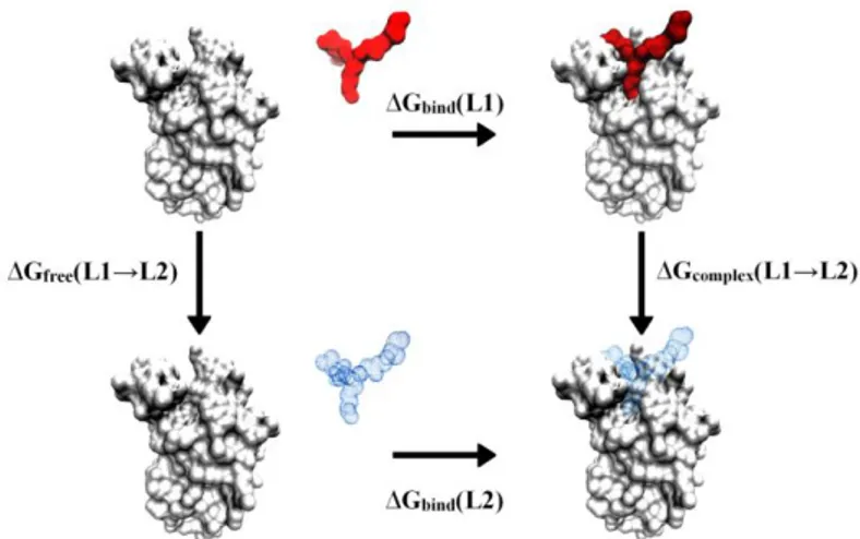
These approaches can be used in a thermodynamic cycle, as illustrated in Figure 1.8, often applied in studying the relative strength of ligand-receptor interactions and the relative stability of proteins differing in one or a few amino acids.

Figure 1.8 Thermodynamic cycle linking the binding of two ligands L1 and L2 to a protein in

solution.

Thermodynamic cycle methods were developed because relatively large, complicated changes need to taken into account when considering the physical phenomena that occur in ligand-receptor binding or the effect of a mutation on protein stability. That is, binding of a drug to a receptor will produce relatively large conformational changes (i.e., the protein will favor a particular set of conformational substates). Binding of a very similar drug to the same site should produce most of the same changes. The thermodynamic cycle is designed to cancel out the large changes that are common to binding of either drug to the receptor.

The horizontal legs describe the experimentally accessible actual binding processes, with free energies ∆Gbind(L1) and ∆Gbind(L2). Since the free energy is a

state function, the relative binding free energy ∆∆Gbind is exactly equal to the

(47)

36

(L1) Equation 1.16

Equation 1.17

The simulations follow the vertical steps (Equation 1.17) or unphysical processes, by simulations in water solution that gradually change the energy-function of the system from one “endpoint” to the other through a series of intermediate hybrid states. From Figure 1.8, this involves the stepwise “alchemical” transformation of ligand L1 to L2 both in its ‘free’ state (unbound) and in the bound complex, through gradual changes in the forcefield parameters describing the ligand interactions. This leads to the free energy changes ∆Gfree(L1→L2) and ∆Gcomplex(L1→L2), respectively. Averaging over both

transformation directions is often used to improve the free-energy estimates, although this is not always the case. These calculations can be accurate, if conducted with the appropriate care.

1.2.3.2 “Endpoint” methods

Although we are assisting on a constant improvement in the computational power, much less computationally demanding “endpoint” methods are often successfully applied, such as the molecular mechanics – Poisson Boltzmann (MM-PBSA) and the related molecular mechanics – generalised Born (MM-GBSA) approximation and the linear interaction energy (LIE). All these methods compute binding free energies along the horizontal legs of Figure 1.8, but use only models for the endpoints (bound and unbound states).

(48)

37

1.2.3.2.1 LIE (Linear Interaction Energy)

The binding of a ligand to a biological macromolecule can be viewed as a process in which the ligand (l) is transferred from one medium, i.e., free in water (f) to another, i.e., the binding site of the water-solvated macromolecular target (b).88

Figure 1.9 Reference state (left) and bound state (right) of a ligand solvated in water

As a consequence, bound state of the ligand and reference state (water-solvated ligand) must be taken into account for a proper description of the total change in free energy associated to the formation of a ligand–receptor molecular complex. This is the correlation behind the LIE method, where the binding free energy is estimated as the free energy of transfer between water and protein environments as:

Equation 1.18

The main difference with respect to a regular transfer process between two solvents is that the standard state in water (1 M and free rotation) is replaced by restricted translation and rotation in a confined receptor-binding site.

(49)

38

In order to calculate the free energy of binding as a solely function of these two physical, relevant states of the ligand, we can draw a thermodynamic cycle (Figure 1.10), where the upper corners represent these two states (left: free, solvated in water; right: bound to the protein). The two bottom corners will account for two unphysical, intermediate states: a pseudo-ligand without any (intermolecular) electrostatic interactions, in its free (left) or bound (right) state.

Figure 1.10 The thermodynamic cycle on which is based the estimation of the binding free energies

with the linear interaction energy (LIE)

The resolution of such a thermodynamic cycle leads to the following equation:

Equation 1.19

where the entropic confinement contributions are hidden in the nonpolar term. Thus, the free energy of binding can be expressed as a sum of the corresponding polar and nonpolar components of the free energy. This is quite convenient, since molecular mechanics force fields analogously split the nonbonded potential energies into electrostatic and nonelectrostatic components. Potential energies (U) can be converted into free energies (∆G) considering that for the polar contribution,