Universit`a di Pisa
Dipartimento di Informatica
Dottorato di Ricerca in Informatica
Ph.D. Thesis
The CIFF Proof Procedure for Abductive Logic
Programming with Constraints: Definition,
Implementation and a Web Application
Giacomo Terreni
Supervisor Paolo Mancarella Supervisor Francesca ToniMay 5, 2008
Abstract
Abduction has found broad application as a powerful tool for hypothetical reasoning with incom-plete knowledge, which can be handled by labeling some pieces of information as abducibles, i.e. as possible hypotheses that can be assumed to hold, provided that they are consistent with the given knowledge base.
Attempts to make the abductive reasoning an effective computational tool gave rise to Abductive
Logic Programming (ALP) which combines abduction with standard logic programming. A number
of so-called proof procedures for ALP have been proposed in the literature, e.g. the IFF procedure, the Kakas and Mancarella procedure and the SLDNFA procedure, which rely upon extensions of different semantics for logic programming. ALP has also been integrated with Constraint Logic
Programming (CLP), in order to combine abductive reasoning with an arithmetic tool for constraint solving.
In recent years, many proof procedures for abductive logic programming with constraints have been proposed, including ACLP and the A-System which have been applied to many fields, e.g. multi-agent systems, scheduling, integration of information.
This dissertation describes the development of a new abductive proof procedure with constraints, namely the CIFF proof procedure. The description is both at the theoretical level, giving a formal definition and a soundness result with respect to the three-valued completion semantics, and at the implementative level with the implemented CIFF System 4.0 as a Prolog meta-interpreter. The main contributions of the CIFF proof procedure are the advances in the expressiveness of the framework with respect to other frameworks for abductive logic programming with constraints, and the overall computational performances of the implemented system.
The second part of the dissertation presents a novel application of the CIFF proof procedure as the computational engine of a tool, the CIFFWEB system, for checking and (possibly) repairing faulty web sites.
Indeed, the exponential growth of the WWW raises the question of maintaining and automatically repairing web sites, in particular when the designers of these sites require them to exhibit certain properties at both structural and data level. The capability of maintaining and repairing web sites is also important to ensure the success of the Semantic Web vision. As the Semantic Web relies upon the definition and the maintenance of consistent data schemas (XML/XMLSchema, RDF/RDFSchema, OWL and so on), tools for reasoning over such schemas (and possibly extending the reasoning to multiple web pages) show great promise.
The CIFFWEB system is such a tool which allows to verify and to repair XML web sites instances, against sets of requirements which have to be fulfilled, through abductive reasoning.
We define an expressive characterization of rules for checking and repairing web sites’ errors and we do a formal mapping of a fragment of a well-known XML query language, namely Xcerpt, to abductive logic programs suitable to fed as input to the CIFF proof procedure.
Finally, the CIFF proof procedure detects the errors and possibly suggests modifications to the XML instances to repair them. The soundness of this process is directly inherited from the sound-ness of CIFF.
Contents
1 Introduction 5
1.1 Abductive Logic Programming and CIFF . . . 6
1.2 CIFF for repairing XML Web sites instances . . . 9
1.3 Overview of the thesis . . . 11
2 Preliminaries 13 2.1 First Order Logic . . . 13
2.1.1 Interpretations and Models . . . 15
2.1.2 Substitutions and unification . . . 17
2.2 Definite Logic Programming . . . 19
2.2.1 Definite clauses, programs and goals . . . 19
2.2.2 Semantics of Definite Logic Programming . . . 20
2.2.3 SLD-resolution . . . 24
2.3 Negation in Logic Programming . . . 27
2.3.1 The Negation As Failure (NAF) rule . . . 27
2.3.2 Completion of a logic program . . . 28
2.3.3 SLDNF for Definite Logic Programs . . . 29
2.3.4 Normal Logic Programming . . . 31
2.3.5 SLDNF resolution for Normal Logic Programs . . . 34
2.4 Alternative Semantics of Normal Logic Programming . . . 35
2.4.1 Three-valued completion semantics . . . 36
2.4.2 Stable models semantics . . . 38
2.4.3 Well-founded semantics . . . 39
2.5 Constraint Logic Programming (CLP) . . . 41
2.6 Answer Sets Programming (ASP) . . . 43
3 Abductive Logic Programming with Constraints (ALPC) 47 3.1 Abductive reasoning . . . 47
3.2 Abduction in logic . . . 48
3.3 Abductive Reasoning in Applications . . . 50
3.4 Abductive Logic Programming (ALP) . . . 51
3.5 Abductive proof procedures . . . 53
3.5.1 The Kakas and Mancarella procedure . . . 53
3.5.2 The SLDNFA procedure . . . 57
3.5.3 The IFF proof procedure . . . 59
3.5.4 Other computational approaches to abduction . . . 62
3.6 ALP + CLP = ALPC . . . 63
3.7 Abductive proof procedures with constraints . . . 65
3.7.1 The ACLP proof procedure . . . 65
4 The CIFF Proof Procedure and the CIFF¬ extension 67
4.1 The CIFF proof procedure . . . 67
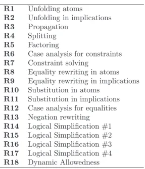
4.1.1 CIFF proof rules . . . 72
4.1.2 CIFF derivation and answer extraction . . . 78
4.2 Soundness of the CIFF Proof Procedure . . . 82
4.3 The CIFF¬ proof procedure . . . . 92
4.4 Soundness of the CIFF¬ proof procedure . . . . 98
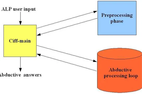
5 The CIFF System 105 5.1 The CIFF System: an Overview . . . 106
5.1.1 Input Programs, Preprocessing and Abductive Answers . . . 109
5.1.2 Variable Handling . . . 113
5.1.3 Constraints Handling . . . 114
5.1.4 Loop Checking and CIFF Proof Rules Ordering . . . 116
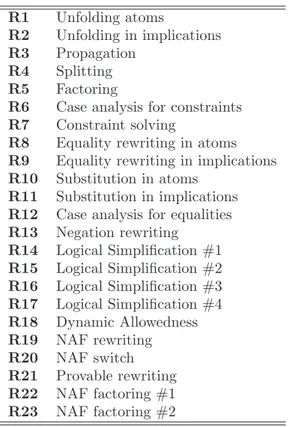
5.1.5 The CIFF¬ proof procedure . . . . 121
5.1.6 Ground Integrity Constraints . . . 123
5.2 Related work and comparison . . . 127
5.2.1 Comparison with A-System . . . . 128
5.2.2 Comparison with Answer Sets Programming . . . 130
5.2.3 Experimental results . . . 132
5.3 Conclusions . . . 139
6 Web Site Verification and Repair 141 6.1 A Motivating Example . . . 142
6.2 A Formal Language for Expressing Web Checking Rules . . . 143
6.3 A Xcerpt-like grammar for positive web checking rules . . . 145
6.4 The translation process for positive rules . . . 146
6.4.1 XML representation . . . 146
6.4.2 The translation function . . . 147
6.5 Adding negation to the translation process . . . 151
6.5.1 Translation function . . . 151
6.6 Analysis for checking . . . 157
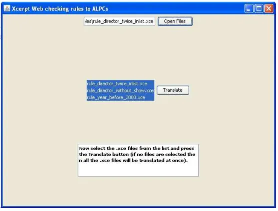
6.7 Running the System . . . 158
6.7.1 A preliminary experimentation . . . 159
6.8 A Web Repairing Framework . . . 160
6.8.1 Abductive logic programs for repairing . . . 161
6.9 Running the CIFFWEB System for repairing . . . 165
6.9.1 Abductively Generated Errors . . . 166
6.10 A more complex running example . . . 167
6.11 Analysis for repairing . . . 168
6.12 Related Work, Future Work and Conclusions . . . 170
6.13 Full theater example . . . 172
6.13.1 XML data . . . 172
6.13.2 XML translation . . . 172
6.13.3 Web checking rules . . . 173
6.13.4 Abductive logic program for checking . . . 178
6.13.5 Abductive logic program for repairing . . . 181
7 Conclusions 185
List of Figures
5.1 The CIFF System: main computational cycle . . . 107
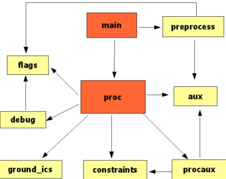
5.2 The CIFF System: modules interactions . . . 110
List of Tables
4.1 CIFF proof rules . . . 81
4.2 CIFF¬ proof rules . . . . 96
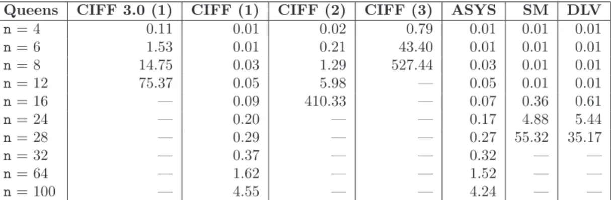
5.1 N-Queens results (first solution) . . . 134
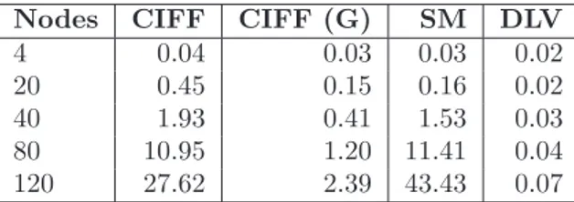
5.2 Hamiltonian cycles results (all solutions) . . . 135
5.3 Graph coloring results (first solution). . . 136
5.4 Scalability results (Test1). . . 137
5.5 Scalability results (Test2). . . 137
5.6 Scalability results (Test3). . . 137
5.7 Scalability results (Test4). . . 138
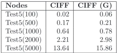
5.8 Scalability results (Test5). . . 138
5.9 Scalability results (Test6). . . 138
Chapter 1
Introduction
Nowadays, computers are massively used in almost every human activity to accomplish an infinite variety of tasks: from intensive data processing to 3D modeling passing through a web search for interesting movies played near home.
This has been a big revolution in modern society and it has been due both to the huge improve-ments in computer hardware in terms of costs, dimensions and performances and the big advances in theoretical computer science whose main applications are the “middlewares” (programming languages, internet protocols and so on) upon which the user-end applications are built.
However, the mostly used “middlewares” (e.g. C and C++ programming languages), to date, allow for writing user-end applications in a machine-oriented language and, on their side, user-end applications are often written to accomplish a specific instance of a more general problem. In the last decade, as the user-end applications have grown in number and complexity, the need emerged of simplifying the building and the maintenance of user-end applications. This need has been even more evidenced by the exponential growth of the World Wide Web which, on the back-end side, needs for computational schemas able to handle huge amounts of heterogeneous data. Thus, a new generation of “middlewares” (e.g. Java and UML) have been developed and used for this purpose.
This generation of commonly used “middlewares”, however, even if improving the previous stage, are still machine-oriented and tailored towards specific user-end applications.
In the meanwhile, almost since the beginning of computer science, a not very popular set of “middlewares” has been developed and refined so far: declarative languages. The main features of a declarative language are to be human-oriented and tailored towards general problem solving. The main idea is that a declarative language provides a formal logic (a well-defined syntax and a clear semantics associated with) plus a control mechanism for that logic (i.e. a “reasoner” which evaluates formulae on that logic), while the application developer has only to model its problem under the logic of the language. It will be the control mechanism inside the language which will evaluate the particular instances of the problem with respect to the given logic.
The straight use of logic for defining the syntax of declarative languages, makes them very suitable tools for knowledge representation, i.e. for representing objects and their relations of the modeled
world in an intuitive human-oriented syntax close to natural langauge. For example in Prolog,
without any doubt the most important and influential example of declarative language which gave rise to the Logic Programming field, to express that a father of a person is a male parent of that
person, it is enough to use the following simple and human-tailored logic formula: f ather(X, Y ) ← parent(X, Y ), male(X)
If we add to the above general statement, the particular “world” instance that John is a male and
John is a parent of Mary, represented as: male(John)
6 CHAPTER 1. INTRODUCTION
the embedded Prolog reasoner is able to deduce that John is the father of M ary.
However, after an initial enthusiasm in the middle 70’s, the popularity of declarative languages shrank dramatically due to the performance gap of declarative applications with respect to hand-tailored applications.
However, there are a number of classic problems and applications which would benefit of a declar-ative approach (planning, scheduling, combinatorial problems) and many other problems which are emerging, in particular concerning the Semantic Web vision. Indeed, the Semantic Web vision relies upon web specification and querying languages (XML/XML Schema, RDF/RDF Schema, OWL, XQuery, XPath, Xcerpt and so on) equipped with a human-tailored logic syntax (plus a not always well-defined semantics). Hence the use of declarative languages as their “control” mechanism is an intuitive, even if non-straightforward choice.
On the other hand, hardware improvements together with the refinements of declarative languages, make the use of them a concrete choice in developing a wide range of applications.
Over the years, declarative languages have been improved in many directions. Prolog itself has been refined and extended in a number of ways. The main extensions of Prolog, enhancing its expressiveness as a tool for knowledge representation, concern parallelism and concurrency (giving rise to distributed logic programming, with communication protocols as typical applications),
arith-metical constraints (giving rise to constraint logic programming, with combinatorial applications
as typical applications) and abduction (giving rise to abductive logic programming, with diagnosis and repairing applications as typical applications).
Our work is placed exactly in this setting, as the main contributions of our thesis are:
• the definition of the CIFF proof procedure, a general-purpose abductive extension of logic programming (including arithmetical constraints) which provides interesting advances in the expressiveness of the abductive framework together with the proof of its soundness with respect to a semantics for logic programming, namely the three-valued completion semantics, • the CIFF System, a robust and efficient implementation, on top of Prolog, of the CIFF proof
procedure, and
• the CIFFWEB System, an automatic tool for detecting and (possibly) repairing errors of XML web sites with respect to web checking rules, i.e. web requirements expressed in Xcerpt, a well-known XML query language with a very human-tailored syntax.
1.1
Abductive Logic Programming and CIFF
The notion of abduction was introduced by the philosopher Pierce in [144] where he identified three main forms of reasoning:
Deduction an analytic process based on the application of general rules to particular cases, with the inference of a result;
Induction synthetic reasoning which infers the rule from the case and the result;
Abduction another form of synthetic inference, inferring the case from a rule and a result. Peirce further characterized abduction as the “probational adoption of a hypothesis” as explanation for observed facts (results) according to known laws. “It is however a weak form of inference, because we cannot say that we believe in the truth of the explanation, but only that it may be true” [144].
Abduction is widely used in common-sense, daily reasoning. For instance in diagnosis, to reason from effect to cause, as noted e.g. in [41].
1.1. ABDUCTIVE LOGIC PROGRAMMING AND CIFF 7
In logic, the abductive task can be formalized as the task of finding a set of hypothesis ∆ which, together with a logic theory P , representing the known laws, allows to infer a set of formulae Q, representing the observations (or the results).
The following well-known example of abductive reasoning was given by Pearl in [141]. Consider to observe that, walking in the garden, the shoes become wet. A simple explanation for this observation is that the grass is wet. Being a sunny day, further explanations are that either the sprinkler was on or it rained during the night. This common-sense process is exactly an abductive process. The explanations have been inferred abductively from the observations and the “rules”, stating for example that “if it rained last night then the grass has to be wet”. A logical formulation of this “world” could be obtained by a theory P consisting of:
grass is wet ← rained last night grass is wet ← sprinkler was on shoes are wet ← grass is wet
In this setting, the observation Q = shoes are wet can be explained by both rained last night and sprinkler was on alternatively.
Typically, in an abductive framework, there is a further component: a set of integrity constraints
IC, i.e. a set of formulae which have to be “satisfied” by ∆ in order to declare such ∆ an acceptable
set of hypothesis for inferring Q. In the above example, an integrity constraint could be
rained last night → f alse
With the above integrity constraint, any abductive explanation containing rained last night is forbidden.
Abduction is a form of nonmonotonic reasoning because explanations which are consistent with an abductive framework, may become inconsistent adding new information to the framework. More formally, the abductive task can be defined as the problem of finding a set of formulae ∆ (abductive explanations for Q) such that:
1. P ∪ ∆ |= Q,
2. P ∪ ∆ is consistent and
3. P ∪ ∆ satisfies IC
where |= stands for a particular logic semantics.
The abductive task can be easily instantiated to logic programming, giving rise to Abductive Logic
Programming (ALP). In general an abductive framework in logic programming is a tuple hP, A, ICi
where P is a logic program, IC is a set of first order closed formulae and A is a set of predicates declared as abducibles. Each atom in ∆ must have a predicate a ∈ A. In the above example the set of abducible predicates is:
A = {rained last night, sprinkler was on}
ALP can also be integrated with Constraint Logic Programming, giving rise to Abductive Logic
Programming with Constraints (ALPC). An abductive framework with constraints is a tuple hP, A, ICi< where < is a constraint structure providing relations and functions (typically arith-metical relations and functions) on a domain D(<), evaluated under the specific semantics of <. In this way an abductive framework with constraints combines the expressiveness of ALP and the expressiveness of the Constraints.
A number of abductive proof procedures for ALP have been proposed in the literature, e.g. the Kakas-Mancarella proof procedure [102, 100], the SLDNFA proof procedure [61] and the IFF proof procedure [82]. Abductive proof procedures, in general, differ in the expressiveness of their specific frameworks and in what rely upon various semantics for logic programming, the most common being the (generalized) stable models semantics [102] and the (three-valued) completion semantics [118].
8 CHAPTER 1. INTRODUCTION
In recent years, several proof procedures for ALPC have also been proposed, including ACLP [109] and the A-System [111].
Abduction (and in particular ALP and ALPC), has been used in a wide range of applications. Abduction can be used to generate causal explanations for fault diagnosis, as seen for example in [147, 56]. In medical diagnosis, for example, the observations are the symptoms and the abductive process finds the possible causes (diseases) of those symptoms [152].
Abduction has been used for improving robotic vision [57, 165] where the observations are the raw data descriptions obtained from the robot visual sensors and the abductive process hypotheses on which objects effectively “see” the robot.
Also scheduling [109] and planning can be easily modeled by means of abduction. A plan can be viewed as a set of hypothetical actions (and subgoals) to be performed (and achieved) in order to reach the final goal state. The main approach to abductive planning is based on the event calculus, a logical framework for reasoning about actions and changes proposed by Sergot and Kowalski in [115]. Abductive planning has been studied by several authors [74, 135, 164].
Database updates is another important application of abduction [170, 101, 19]. In this setting
the observations are the update requests and the abductive explanations are the transactions that satisfy those requests.
Finally, in recent years, abduction has been studied has a main reasoning paradigm for modeling
intelligent and autonomous agents, a field that has captured great attention in the last decades
[148, 53, 149, 98, 105, 31]. An intelligent agent can be defined as an actor which is capable of observing, reasoning and acting upon a (dynamical) environment.
The main contribution of this thesis is the CIFF proof procedure for ALPC. CIFF (see [71, 72, 70, 125, 73] for preliminary versions and applications) is a proof procedure based on rewriting, i.e. its computational core is based on a set of proof rules which rewrite a formula into an equivalent formula under the three-valued completion semantics. CIFF is an extension of the IFF proof procedure [82], which, with respect to other abductive proof procedures, shows two main features: (1) handling of (existentially and universally quantified) variables and (2) handling of integrity constraints in implicative form:
L1∧ · · · ∧ Lm → A1∨ · · · ∨ An.
This form of integrity constraint makes possible the use of forward reasoning in addition to the classical Prolog-style backward reasoning, allowing for a flexible computational tool for modeling a wider class of problems. In particular forward reasoning with integrity constraints in implicative form can capture the condition-action rule type of behavior, which is very typical and useful in dynamic settings [157].
The CIFF proof procedure extends IFF in three ways, namely (1) by integrating abductive rea-soning with constraint solving, (2) by relaxing the allowedness conditions on suitable inputs given in [82], in order to be able to handle a wider class of problems, and (3) by adding a different type of negation treatment in integrity constraints, namely the negation as failure (NAF) [48].
The third extension was similarly proposed in [157] as an extension for the IFF proof procedure. To briefly explain the NAF extension let us consider a very simple integrity constraint like the following:
¬L → A.
Normally, in CIFF, the negation is treated as classical negation, and the IC is treated equivalently to the disjunction A ∨ L. Hence, in order to satisfy the IC either A or L must hold. However, often such an IC is required to produce condition-action or reactive behavior, where the intended interpretation is:
if there is evidence that ¬L holds, then A must hold too,
1.2. CIFF FOR REPAIRING XML WEB SITES INSTANCES 9
if there is no evidence that L holds, then A must hold.
This is exactly what the NAF view allows, avoiding some unintuitive abductive answers. Consider a “world” where an agent has to clean in a dangerous environment. The idea is that if it is a cleaning day and the alarm has not been activated, the agent must dust. This could be represented by the integrity constraint
cleaning day ∧ ¬sound alarm → dust
A logical interpretation of negation, provided that today is a cleaning day, allows the agent to either dust or sound the alarm (even if no dangerous situation arises) in order to satisfy its rule of behavior! In the NAF view, the agent avoids to dust only if the alarm has been sounded for some other reason. As we will see, this feature enhances the expressive power of the framework especially for modeling condition-action and reactivity rules.
A main contribution of this thesis, is also the proof of soundness of CIFF with respect to the three-valued completion semantics.
The CIFF proof procedure has been implemented in Prolog in the CIFF System, which is available at www.di.unipi.it/∼terreni/research.php.
The system is a mature Prolog system for which much time has been spent in exploiting Prolog algorithms and data structures for improving the overall efficiency of the system, but maintaining a clear mapping between the specification and the implementation.
We have compared empirically CIFF and the CIFF System to other related systems, namely the A-System [111, 139], that is the closest system from both a theoretical and an implementative viewpoint, and two state-of-the-art answer sets solvers SMODELS [136, 166] and DLV [68, 119]. Answer sets solvers are very popular tools which implement the (answer sets) semantics [90]. Their computational schema is very distinct from the computational schema of logic programming and they gave rise to the branch of Answer Sets Programming (ASP). However, ASP shares with ALPC the objective of modeling dynamic and non-monotonic settings in a declarative (and thus human-oriented) way.
The comparison both evidences how CIFF enriches the expressiveness of the abductive framework and both evidences the similarities and the differences between ALPC and ASP. In particular we outline how CIFF, with its NAF extension, is a step towards a unifying framework for ALPC and ASP.
The experimental results on the CIFF System show that (1) the CIFF System and the other systems have comparable performances and (2) the CIFF System has some unique features, e.g. its incorporation of NAF in integrity constraints and its handling of variables taking values on unbound domains.
The features of earlier versions of the procedure have been exploited in various application domains. In [105] CIFF has been used as the computational core for modeling an agent’s planning, reactivity and temporal reasoning capabilities, based on a variant of the abductive event calculus [115, 133]. A prototype version of the CIFF system has also been studied for abductive planning [124, 71].
1.2
CIFF for repairing XML Web sites instances
We strongly believe that declarative languages such as Prolog [54], if they are well integrated with the web, will play a crucial role as the computational paradigms in the Semantic Web vision, as noted, e.g., in [182].
The increasing interest about the Semantic Web technologies [175, 13] seems to be the right place for declarative approaches. In particular web specification languages from XML/XMLSchema [177] to OWL [176] passing through RDF/RDFSchema [174] need expressive computational counterparts allowing more and more reasoning capabilities.
10 CHAPTER 1. INTRODUCTION
Abduction too, as it is a very suitable form of reasoning for diagnosis and repairing, could play a prominent role in that context, as noted, e.g., in [39], where some abductive tasks over ontologies have been individuated.
In this thesis we concentrate on how abduction could be used as a computational mechanism for maintaining and repairing XML/XHTML web sites instances.
The exponential growth of the WWW raises the question of maintaining and automatically re-pairing web sites, in particular when the designers of these sites require them to exhibit certain properties at both structural and data level. The capability of maintaining and repairing web sites is also important to ensure the success of the Semantic Web [175, 13] vision. Nevertheless, there is limited work on specifying, verifying and repairing web sites at a semantic level. Notable exceptions, at least for specifying and checking web sites, are represented by works such as [173] (which mainly inspired our work) [62] and [78]; the XLINKIT framework [40] and the GVERDI-R system [10, 23].
Searching the web, it is easy to encounter web pages containing errors in their structure and/or their data. We argue that, in most cases, considering an XML/XHTML web site instance, the errors can be divided into two main categories: structural errors and content-related (data) errors. Structural errors are those errors concerning the presence and/or absence of tag elements and relations amongst tag elements in the pages. For example, if a tag tag1 is intended to be a child of a tag tag2, the occurrence in the web site of a tag1 instance outside the scope of a tag2 instance is a structural error. Data errors, instead, are about the in-tag data content of tag elements. For example a tag3 could be imposed to hold a number greater than 100.
Consider the following extracts of two XML pages, representing, in a theater company web site instance, a list of shows produced by that company and the list of directors of that company:
%%%directorindex.xml %%%showindex.xml <directorlist> <showlist> <director>John</director> <show> <director>Mary</director> <showname>Epiloghi</showname> </directorlist> <year>2001</year> </show> </showlist>
We could specify a number of rules which any web site instance should fulfill. For example, we could specify that a correct structure of a show tag in the first page must contain both a showname tag element and a dir by tag element as its child. In this case we have a structural error, due to the lack of a dir by tag element in the show of the list. Also, we could specify that all the shows in the list must be produced since the year 2000. In this case we have a data error if the value inside an year tag is less than 2000.
Requirements (and thus errors) can involve more than one web page. For example, a possible requirement for the theater company specification may be that
each director must direct at least one show
The above requirement can lead to content-related errors which involve both pages because the
content of each director tag, e.g. John has to be matched to the content of at least one dir by
tag inside a show tag.
Here, we propose the CIFFWEB (prototype) tool, which, roughly speaking, uses CIFF as the computational core for verifying and, possibly, repairing web sites against sets of requirements which have to be fulfilled by a web site instance. A preliminary version of the tool is shortly described in [127].
We argue that the CIFF proof procedure has very useful features to be applied in a web reasoning scenario: implicative integrity constraints which could act as condition-action rules, handling of unbound variables which could directly represent missing data, and arithmetical constraint solving capabilities.
1.3. OVERVIEW OF THE THESIS 11
In our framework, we define an expressive characterization of rules for checking web sites’ errors by using (a fragment of) the well-known semi-structured data query language Xcerpt [37, 38]. With respect to the other semi-structured query languages (like XQuery [27], XPath [47]) which all propose a path-oriented approach for querying semi-structured data, Xcerpt is a rule-based language which relies upon a (partial) pattern matching mechanism allowing to easily express complex queries in a natural and human-tailored syntax. Xcerpt shares many features of logic programming, for example its use of variables as place-holders and unification. However, to the best of our knowledge, it lacks (1) a clear semantics for negation constructs and (2) an implemented tool for running Xcerpt programs and evaluating Xcerpt queries. A by-product of this Chapter is the provision of both (1) and (2) for a fraction of Xcerpt, namely the subset of this language that we adopt for expressing web checking rules.
Then, we map formally the chosen fragment of Xcerpt for expressing checking rules into programs
for checking, i.e. abductive logic programs with constraints that can be fed as input to the
general-purpose CIFF proof procedure. By mapping web checking rules onto abductive logic programs with constraints and deploying CIFF for determining fulfillment (or identify violation) of the rules, we inherit the soundness properties of CIFF thus obtaining a sound concrete tool for web checking. At the end of the translation process the CIFF System can be successfully used to reason upon the (translation of the) web checking rules finding those XML/XHTML instances not fulfilling the rules, and representing errors as abducibles in abductive logic programs. The CIFFWEB tool also integrates a JAVA translator from web checking rules to both programs for checking and program for repairing.
However, abductive reasoning seems to be very suitable not only for identifying errors in a web site instance but also for suggesting possible repair actions for them. In this respect, abducibles may represent not only an error instance fired by an XML/XHTML instance violating a rule r (for checking) but also possible modifications (repairs) to that XML/XHTML data such that both r is fulfilled and no other rules are violated.
Following these observations, we have identified some type of errors, arising from the violation of web checking rules, which are suitable for abductive repair, and we have done a further mapping from web checking rules to another type of abductive logic program with constraints: programs
for repairing. Again, we use programs for repairing as input for CIFF which either determines
the fulfillment of the rules, or for suggesting appropriate repair actions. The soundness properties of CIFF are inherited also in the repair framework, thus obtaining a sound concrete tool for web repairing.
To our knowledge, the repairing feature is a novel feature with respect to the other existing tools for web verification.
1.3
Overview of the thesis
The first two chapters of the thesis contain background notions. In Chapter 2 we present a brief overview of Logic Programming, considering its extensions and its alternatives related to our work. The abductive extension of Logic Programming, i.e. ALP, is left as the subject of Chapter 3, where we present a brief overview of the various abductive approaches in the literature, including several abductive proof procedures (with constraints).
Chapter 4 is arguably the main chapter of the thesis: the CIFF proof procedure, together with its NAF extension, is formally defined and its soundness with respect to the three-valued completion semantics is proved.
In Chapter 5, the CIFF System is described, pointing out the main algorithms and data structures used in order to make the system efficient. This chapter ends with a comparison of CIFF, both at theoretical and at implementative level, with other, related, existing tools.
The CIFFWEB tool for web sites verification and repair is the main subject of Chapter 6. The web checking rules are formally defined as well as the translation function to abductive logic programs with constraints.
12 CHAPTER 1. INTRODUCTION
Chapter 2
Preliminaries
This chapter summarizes the basic background about Logic Programming (LP) which, roughly speaking, can be described as the application of (a part of) mathematical logic in computer pro-gramming. In this view of logic programming, which can be traced at least as far back as John McCarthy’s advice-taker proposal [130], logic is used as a purely declarative representation lan-guage, and a theorem-prover or model-generator is used as the problem-solver.
Fifty years of research have produced a large amount of logic-based formalisms to improve both the computational aspect of logic programming and its expressiveness. Surely, the most influential result, which made logic programming as it is understood nowadays, was the definition of the Prolog language [54, 116].
Since the birth of Prolog, logic programming has been extended in so many ways that a compre-hensive survey of the logic programming is almost an impossible task. Abductive logic programming (ALP) which is the central field of this thesis is such an extension of logic programming and it will be described in detail in the next chapter. In this chapter we focus on the core of logic programming, briefly describing its foundations and the extensions which are closer to our work. We introduce first order languages together with the notions of interpretations and models of first order theories. In sections 2.2 and 2.3 we introduce logic programming, defining its syntax and its classical semantics. Then we present the most influential alternative semantics for negation in logic programming. Section 2.5 briefly introduces an important extension of logic programming, namely Constraint Logic Programming (CLP). Finally we present a short overview of a distinct Logic Programming framework, namely Answer Sets Programming (ASP). For a detailed overview on these subjects, refer to [123], [118], [17], [88], [94], [87].
2.1
First Order Logic
First order logic has two basic aspects: syntax and semantics. We start defining the syntax, i.e. defining a first order language.
A first order language is based upon a signature (or an alphabet), which is defined as follows.
Definition 2.1. A signature is composed of the following classes of symbols:
1. Variables: we denote variables by X, Y, Z... 2. Constants: we denote constants by a, b, c...
3. Function symbols: we denote function symbols by f, g, h...
4. Predicate (or relation) symbols: we denote predicate symbols by p, q, r... 5. Two special symbols: true and false
14 CHAPTER 2. PRELIMINARIES
6. Connectives: ¬ (negation), ∨ (disjunction), ∧ (conjunction), →(implication), ↔
(equiva-lence)
7. Quantifiers: ∃ (there exists), ∀ (for all) 8. Punctuation symbols: ’(’, ’)’, ’[’, ’]’, ’,’.
2
The sets of connectives, quantifiers, punctuation symbols and the two special symbols are fixed. We assume that the set of variables is infinite and also fixed. These classes of symbols are called
logical symbols. Constants, function symbols and predicate symbols may vary and they are called non-logical symbols. A first-order language is determined by its non-logical symbols. In this thesis
we also assume that the set of function symbols in a first-order language is infinite unless stated explicitly otherwise.
Each function symbol and predicate symbol has a fixed arity, that is the number of its arguments. A function (predicate) symbol with n arguments is said to be a n-ary function (predicate) symbol. Constants can be regarded as 0-ary function symbols.
An important class of strings of symbols over a given alphabet is the class of terms.
Definition 2.2. A term is:
1. a variable,
2. a constant, or
3. a compound term f (t1, . . . , tn) where f is a n-ary function symbol and t1, . . . , tn are terms.
2
A tuple of variables X1, X2, X3. . . (resp. terms t1, t2, t3. . .) is denoted as ~X (resp. ~t). For example
f (~t) is a shorthand for f (t1, . . . , tn).
Over the class of terms is built the class of formulas.
Definition 2.3. A formula is:
1. a special symbol ( true or false),
2. p(t1, . . . , tn) where p is a n-ary predicate symbol and t1, . . . , tn are terms, 3. φ ∨ ψ, φ ∧ ψ, φ → ψ, φ ↔ ψ, ¬φ, where φ, ψ are formulae,
4. ∃X.φ and ∀X.φ where φ is a formula and X is a variable.
We say that a formula of the first two categories is an atomic formula or simply an atom. A literal is either A or ¬A, A being an atom. A positive literal is an atom. A negative literal is the negation of an atom.
Given a literal L, we denote by P red(L) the n-ary predicate of L. 2
We are ready to give the formal definition of first order language.
Definition 2.4. A first order language L based on a given alphabet A is the set of all the formulae
that can be constructed from that alphabet. 2
A formula or a term are called ground when they contain no variables. If they contain at least a variable they are called non-ground.
In a formula ∃X.φ (respectively ∀X.φ), the quantifier ∃ (resp. ∀) binds X in φ. The scope of ∃X (resp. ∀X) is defined to be φ. A variable in a formula φ which is not bound by a quantifier is called a free variable.
2.1. FIRST ORDER LOGIC 15
Definition 2.5 (Closed formula). A formula φ is closed when there is no free variable X occurring in φ. Let X1, . . . , Xn be the free variables in a formula φ, we write ∃(φ) for ∃X1, . . . , ∃Xn(φ) (the existential closure of φ) and we write ∀(φ) for ∀X1, . . . , ∀Xn(φ) (the universal closure of φ). A
closed formula is also called a sentence. 2
Definition 2.6 (Theory). We define a theory T of a first order language L as a set of closed
formulae of L. Each formula F ∈ T is called an axiom. 2
2.1.1
Interpretations and Models
The semantics of first orders logic relies upon the concepts of interpretations and models which give the meaning to formulae of first order languages.
Definition 2.7 (Pre-interpretation).A pre-interpretation J of a first order language L is composed of:
• a non-empty set of objects D called the domain of J,
• a set JC containing, for each constant in L, an assignment of an element in D,
• a set JF containing, for each n-ary function symbol in L, a mapping from Dn to D. When needed, we write JD to highlight the domain D of the pre-interpretation J. 2
Definition 2.8 (Interpretation). An interpretation I of a first order language L consists of a pre-interpretation JD of L together with a set IP containing, for each n-ary predicate symbol in L, a mapping from Dn to the set {true, f alse}. We also say that I is based on JD 2
Definition 2.9 (Variable assignment). Let JD be a pre-interpretation of a first order language L. A variable assignment α with respect to J assigns an element in D to each variable in L.
Given a formula F of L, we denote by F [X 7→ d] the formula F0 of L obtained by replacing all the
occurrences of the variable X in F by the domain element d. 2
Definition 2.10 (Semantics of terms). Let I be an interpretation (based on JD) of a first order language L, let α be a variable assignment and let t be a term. The meaning αIof t is defined as follows:
• if t is a constant c ∈ L then αI(t) = JC(c),
• if t is a variable X ∈ L then αI(t) = α(X),
• if t is a compound term f (t1, . . . , tn) then αI(t) = fJ(αI(t1), . . . , αI(tn)), where fJ= JF(f )
Notice that the semantics of a compound term is obtained by applying the function fJ to the
meanings of its principal subterms, which are obtained by recursive application of the above defi-nition.
We introduce now the semantics of formulae of a first order language L which associates a formula
F to a truth value (true, f alse). In the following definition, the notation I |=α Q means “Q is true with respect to the interpretation I and the variable assignment α”. In the same way I 6|=αQ
means “Q is f alse with respect to the interpretation I and the variable assignment α”.
Definition 2.11 (Semantics of formulae). Let I be an interpretation (based on JD) of a first order language L and let α be a variable assignment. The meaning of a formula Q ∈ L is defined as follows:
• for each n-ary predicate symbol p ∈ L, given pI = IP(p), we have that:
16 CHAPTER 2. PRELIMINARIES – I 6|=αQ = p(t1, . . . , tn) iff pI(αI(t1), . . . , αI(tn)) = f alse • I |=αQ = (¬F ) iff I 6|=αF • I |=αQ = (F ∧ G) iff I |=αF and I |=αG • I |=αQ = (F ∨ G) iff I |=αF or I |=αG • I |=αQ = (F → G) iff I 6|=αF or I |=αG • I |=αQ = (F ↔ G) iff I |=α(F → G) and I |=α(G → F )
• I |=αQ = (∀X.F ) iff I |=α[X7→d]F for each d ∈ D
• I |=αQ = (∃X.F ) iff I |=α[X7→d]F for some d ∈ D where F, G are formulae in L and X is a variable in L.
2
It is easy to see that the semantics of a closed formula does not depend on a variable assignment
α, but it depends only on the interpretation I. Hence, we can speak unambiguously of a semantics
of a closed formula Q with respect to an interpretation I. I.e. we denote by I |= Q (resp. I 6|= Q) the fact that a closed formula Q is true (resp. f alse) with respect to an interpretation I.
The introduction of the syntax and the semantics of formulae of a first order language L allows us to have a tool for describing and characterizing “worlds”. While the language L describes the universe of a discourse, a “world”, it is natural to ask whether a set S of closed formulae and an interpretation I give a proper account of this “world”. This is the case if all the formulae of S are true with respect to I.
Definition 2.12 (Model). Let S be a set of closed formulae of a first order language L. We say that M is a model of S if M is an interpretation of L such that for each formula F ∈ S:
M |= F
We denote that M is a model for S by M |= S and that M is not a model for S by M 6|= S. 2
Obviously there are infinitely many interpretations I for language L. However it may happen that none of them is a model of a set of closed formulae S (e.g. S = F ∧ ¬F ). Conversely, it may happen that all of them are models of S (e.g. S = F ∨ ¬F ). We have the following classification of sets of closed formulae S.
Definition 2.13. Let S be a set of closed formulae of a first order language L. We say that
• S is consistent1 if there exists an interpretation I of L such that I |= S, • S is valid if for every interpretation I of L, I |= S,
• S is inconsistent if there is no interpretation I of L such that I |= S,
• S is nonvalid if there exists an interpretation I of L such that I 6|= S.
2
Given a set of closed formulae S, it is also interesting to characterize formulae F which can be “derived” from S. I.e. formulae F that are true in every model of S. This is the idea behind the concept of logical consequence.
1We use the word consistent and not satisfiable as the literature on Logic Programming generally does, because
2.1. FIRST ORDER LOGIC 17
Definition 2.14 (Logical Consequence). Let S be a set of closed formulae and F be a closed formula of a first order language L. We say that F is a logical consequence of S (denoted again as S |= F ) if, for every interpretation I of L, we have that:
if (I |= S) then (I |= F )
2
Proposition 2.1. Let S be a set of closed formulae and F be a closed formula of a first order language L. Then F is a logical consequence of S if and only if S ∪ {¬F } is inconsistent. 2
Another important concept about the semantics of formulae is the concept of logical equivalence.
Definition 2.15 (Logical Equivalence). Let F and G be two formulae. We say that F and G are
logically equivalent (denoted by F ≡ G) if and only if F and G have the same truth value for each
interpretation I and variable assignment α. 2
2.1.2
Substitutions and unification
In this section we present two fundamental concepts which are the basis of the operational mech-anisms in Logic Programming: substitutions and unification.
Definition 2.16 (Substitution). A substitution σ is a finite set of the form {X1/t1, . . . , Xn/tn}
where each Xi is a variable (distinct from each other) and each ti is a term distinct from Xi. Each element X1/t1 is called a binding for Xi. If all the ti are ground terms, then σ is called a ground substitution. The substitution given by the empty set is called the empty substitution and
is denoted as ². 2
Definition 2.17. An expression E is either a term or a formula. A simple expression is either a term or an atom.
Definition 2.18 (Instance). Let σ = {X1/t1, . . . , Xn/tn} be a substitution and let E be an ex-pression. The expression Eσ is called the instance of E by σ and it is obtained by simultaneously replacing each occurrence of all the variables X1, . . . , Xnin E by the corresponding terms t1, . . . , tn.
An instance containing no variables is called a ground instance. 2
Definition 2.19 (Variant). Let E and F be expressions. We say that E and F are variants if there exist substitutions σ and θ such that E = F σ and F = Eθ. We also say E is a variant of F and F is a variant of E.
2
Substitutions can be composed and they have elementary properties as follows.
Definition 2.20. Let σ = {X1/t1, . . . , Xn/tn} and θ = {Y1/v1, . . . , Ym/vm} be substitutions. The composed substitution σθ is defined as the set:
{Xi/tiθ | i ∈ [1 . . . n] ∧ Xi6= tiθ} ∪ {Yj/vj | j ∈ [1 . . . m] ∧ Yj6∈ {X1, . . . , Xn}}
2
Proposition 2.2. Let σ, θ, γ be substitutions and let E be an expression. The:
• σ² = ²σ = σ
• (Eσ)θ = E(σθ) • (θσ)γ = θ(σγ)
18 CHAPTER 2. PRELIMINARIES
Example 2.1. The followings are simple examples of substitutions: p(f (X, Z), f (Y, a)){X/a, Y /Z, W/b} = p(f (a, Z), f (Z, a))
p(X, Y ){X/f (Y ), Y /b} = p(f (Y ), b)
The following, instead, is a simple example of a composition of substitutions: {X/f (Z), Y /W }{X/a, Z/a, W/Y } = {X/f (a), Z/a, W/Y }
2
Substitutions are needed for defining a central procedural mechanism of logic programming:
uni-fication.
Definition 2.21. Let S be a set of simple expressions and let be σ a substitution. σ is a unifier of S if Sσ is a singleton. σ is the most general unifier (mgu) for S if and only if for each unifier
θ of S, there exists a substitution γ such that θ = σγ. 2
The search of a unifier (and in particular an mgu) of two expressions E and F , can be viewed as the process of solving the equation E = F . More generally, given a set of equations {E1= F1, . . . , En=
Fn}, θ is a unifier of this set if Eiθ = Fiθ for each i ∈ [1, n]. For example θ = {X/a, Y /a} is a
unifier of the equation f (X, g(Y )) = f (a, g(X)).
Here we present the Martelli-Montanari algorithm [129] for finding an mgu of a set of equations. It is based on the concept of equations in solved form.
Definition 2.22. A set of equations {X1= t1, . . . , Xn = tn} is in solved form if X1, . . . , Xn are
distinct variables none of which appear in t1, . . . , tn. 2
A set of equations in solved form has the following interesting property, whose proof can be found in [137].
Proposition 2.3. Let {X1 = t1, . . . , Xn = tn} be a set of equations in solved form. Then
{X1/t1, . . . , Xn/tn} is an mgu of the solved form. 2
It is also important to introduce the concept of equivalence between sets of equations.
Definition 2.23. Two sets of equations are said to be equivalent if they have the same set of
unifiers. 2
The Martelli-Montanari algorithm, given a set of equations, gives out (if possible) an equivalent set of equations in solved form. It is clear that, by definition of two equivalent sets of equations, an mgu of the solved form is also an mgu of the non-solved form.
Definition 2.24. [Unification Algorithm] Input: a set of equations S0.
begin S := S0 repeat select an arbitrary s = t in S case s = t of (1) f (s1, . . . , sn) = f (t1, . . . , tn): replace by s1= t1, . . . , sn= tn (2) f (s1, . . . , sn) = g(t1, . . . , tm): fail
(3) X = X: delete the equation
(4) t = X where t is not a variable: replace by X = t
(5) X = t where X does not occur in t and X appears elsewhere in S: replace all the occurrences of X in S by t
2.2. DEFINITE LOGIC PROGRAMMING 19
(6) X = t where X 6= t and X occurs in t: fail. until no action is possible in S
end Output: S
2
The following theorem states the soundness and the completeness of the above unification algo-rithm, see [137] for the proof.
Theorem 2.1 (Unification Theorem). Let S be a set of equations. The unification algorithm of definition 2.24 applied on S terminates and returns an equivalent solved form of S of failure if no
such solved form exists. 2
Example 2.2. The following set {f (X, g(Y )) = f (g(Z), Z)} has a solved form, indeed: {f (X, g(Y )) = f (g(Z), Z)} ⇒ (1)
{X = g(Z), g(Y ) = Z} ⇒ (4) {X = g(Z), Z = g(Y )} ⇒ (6) {X = g(g(Y )), Z = g(Y )}
The following set {f (X, g(X)) = f (Z, Z)}, instead, does not have a solved form: {f (X, g(X)) = f (Z, Z)} ⇒ (1)
{X = Z, g(X) = Z} ⇒ (4) {X = Z, Z = g(Z)} ⇒ (5) fail
This is because Z is a proper subterm of g(Z). 2
2.2
Definite Logic Programming
The very basic idea behind Logic Programming is to use a computer to draw conclusions from declarative descriptions. Those descriptions, called logic programs, consist of finite sets of logic formulae. In order to achieve logic systems which exhibit interesting theoretical properties and which could be computationally attractive, it was clear that restrictions on the logic formulae were needed.
In this section we introduce the language of the definite logic programs which is the core of logic programming as it is intended today. The main limitation in a definite logic program is the lack of
negation: only positive “objects” can be described. The absence of negation, however, allows the
definition of a clear and universally accepted declarative semantics for definite logic programs: the
least Herbrand model semantics as well as its procedural counterpart: the SLD-resolution [116].
2.2.1
Definite clauses, programs and goals
A particular type of declarative sentence describing both facts and rules about a domain and which is used to compose logic programs is the clause. In particular we restrict our attention to definite
clauses.
Definition 2.25 (Definite clause). A definite clause is a a first order formula of the form: ∀(H ∨ ¬A1∨ . . . ∨ ¬An)
where H and each Ai are atoms. A definite clause can be represented in implicative form (we use the notation ← instead of → for convenience) as follows:
20 CHAPTER 2. PRELIMINARIES
H ← A1, . . . , An
.
2 H is called the head of the clause and B = L1, . . . , Ln the body of the clause. The empty head is equivalent to f alse whereas the empty body is equivalent to true. In the first case we say that the clause is a denial whereas in the latter case we say that the clause is a fact. The empty clause is denoted as 2.
Definition 2.26 (Definite Logic Program). A definite logic program is a finite set of definite
clauses. 2
Example 2.3. Let us consider the following sentences:
1. John is a parent of Mary
2. John is a male person
3. A father of a person is a male and he is a parent of that person. The following definite logic program can be used to express above sentences.
parent(john, mary). male(john).
f ather(X, Y ) ← parent(X, Y ), male(X). 2
A logic program is a description of a “world” and it is used to draw conclusions about it, i.e. it is used to determine whether a certain sentence is a logical consequence of the program or not. In logic programming such a sentence is in the form of a goal.
Definition 2.27. [Definite Goal] A definite goal (or a definite query) G is a clause of the form: ← A1, . . . , An
where each Ai is an atom and it is called a subgoal of G. 2
In the sequel we will drop the word “definite” if it is clear from the context.
Example 2.4. Consider the example 2.3. The goal ← f ather(john, mary)
is a logical consequence of the program. 2
2.2.2
Semantics of Definite Logic Programming
As noted in the previous section, logic programs are used to check whether a goal is a logical consequence of a program or not. Thus, it is natural to characterize the declarative semantics of a logic program as the set of its logical consequences. In the case of definite logic programming, where both logic programs and goals are definite, it is possible to characterize such a set as the
least Herbrand model. Furthermore, there is also an operational (or procedural) semantics that
has been defined for definite logic programming: it is based on the SLD-resolution [116] principle. Both semantics are universally accepted as the “correct” semantics for definite logic programming and an equivalence result between the two has been shown. For further details and all the proofs of propositions and theorems in this section see, for example, [123, 137, 14].
2.2. DEFINITE LOGIC PROGRAMMING 21
The least Herbrand model semantics
The least Herbrand model semantics is based upon a special class of models of definite logic pro-grams: the class of Herbrand models. The idea is to abstract from the actual meanings of the functors and the constants (0-ary functors) of the language and to focus on those interpretations (Herbrand interpretations) whose domain is the set of variable-free terms and the meaning of a ground term is the term itself.
Definition 2.28 (Herbrand Universe). Let L be a first order language. The Herbrand Universe UL of L is the set of all ground terms which can be constructed out from the function symbols and
the constants of L. 2
Definition 2.29 (Herbrand Base). Let L be a first order language. The Herbrand Base BL of L is the set of all ground atoms which can be constructed from the predicate symbols and the ground
terms in UL. 2
Both Herbrand universe and Herbrand base are usually defined over a given logic program P . In this case it is assumed that the alphabet of the language is composed exactly of those symbols appearing in P .
Example 2.5. Let us consider the following logic program PODD: odd(s(0)).
odd(s(s(X))) ← odd(X).
In this case the Herbrand universe UP and the Herbrand base BP look as follows: UP = {0, s(0), s(s(0)), . . .}
BP = {odd(0), odd(s(0)), odd(s(s(0))), . . .}
2
Definition 2.30. [Herbrand Pre-interpretation and Herbrand Interpretation] A Herbrand
pre-interpretation J for a first order language L is the pre-pre-interpretation of L defined as follows: • the domain is the Herbrand Universe UL,
• JC is the identity function for each c ∈ L,
• JF is the mapping Un
L 7→ UL : (t1, . . . , tn) 7→ f (t1, . . . , tn), for each n-ary function symbol f
in L.
A Herbrand interpretation I for a first order language L is any interpretation based on the Herbrand
pre-interpretation J for L. 2
Thus, Herbrand interpretations for a logic program P have fixed meanings for the constants and the functors: in order to specify a Herbrand interpretation I it suffices to list, for each n-ary predicate symbol p in P , the n-tuples ht1, . . . , tni of ground terms such that I |= p(t1, . . . , tn). In practice an Herbrand interpretation is a subset of the Herbrand base BP.
Example 2.6. The followings are Herbrand interpretations for the logic program P in the example 2.5: I1 = {®} I2 = {odd(s(0))} I3 = {odd(sn(0)) | n ∈ {1, 3, 5, 7, . . .}} I4 = {BP} 2
22 CHAPTER 2. PRELIMINARIES
Definition 2.31 (Herbrand Model). A Herbrand model M for a set of closed formulae S of a first order language L is a Herbrand interpretation I for L such that:
M |= S
2
Example 2.7. Consider again the examples 2.5 and 2.6. The Herbrand interpretation I1 is not a
Herbrand model for P since odd(s(0)) is not true in I1. Conversely I4= BP is clearly a Herbrand model for P . Let us consider I2. It is not a model of P because there is a ground instance of the
rule odd(s(s(X))) ← odd(X), namely odd(s(s(s(0)))) ← odd(s(0)), such that all the premises are true. However odd(s(s(s(0)))) is not belonging to I2. Finally I3 is a Herbrand model of P . Indeed
odd(s(0)) is true in I3. Let us consider any ground instance odd(s(s(t))) ← odd(t) of the rule, with
t ∈ UP. If odd(t) 6∈ I3 the ground instance is obviously true. Otherwise we have that obviously
also odd(s(s(t))) ∈ I3 by definition. 2
In the above example I4= BP was a Herbrand model of P . Indeed, for each logic program P , BP
is a Herbrand model because it contains all the ground instances of each predicate of P . However, by its definition, BP is not an “interesting” model. An interesting model should not contain more
instances of those which effectively follow from a program P . This interesting model is the least
Herbrand model, which characterizes the semantics of a definite logic program.
We have the following interesting property about Herbrand models.
Proposition 2.4. Let P be a definite logic program and let M be a non-empty set of Herbrand models for P . Then the intersection MP of all the Herbrand models in M is an Herbrand model. 2
Definition 2.32. The least Herbrand model MP of a logic program P is the intersection of all
the Herbrand models of P . 2
Example 2.8. The least Herbrand model of the program P in the example 2.5 is the Herbrand interpretation I3 seen in the example 2.6 i.e.:
I3= {odd(sn(0)) | n ∈ {1, 3, 5, 7, . . .}} 2
The fact that the least Herbrand model MP contains effectively all the elements of BP which follow
from P was shown by Kowalski and Van Emden in [69] which characterized MP as the set of all
the logical consequences of P .
Theorem 2.2. Let P be a definite logic program (with Herbrand base BP). Then MP = {A ∈ BP | P |= A}
2
There is also a constructive characterization of the least Herbrand model which we present now.
Definition 2.33 (Grounded Logic Program). Let P be a logic program, we define the grounded
logic program ground(P ) as the logic program obtained by replacing all the non-ground clauses of
P by all their ground instances. 2
Let us consider the set H of all the Herbrand interpretations of a logic program P . We introduce the immediate consequence operator.
Definition 2.34 (Immediate Consequence Operator). Let P be a definite logic program and let I be a Herbrand interpretation of P . The mapping TP : H 7→ H is defined as follows:
TP(I) = {A | A ← A1, . . . , An∈ ground(P ) and A1, . . . , An⊆ I}
2.2. DEFINITE LOGIC PROGRAMMING 23
To clarify the interest of TPwe need to (very briefly) recall the fixpoint theory. Further information
on this topic can be found for example in [123, 169].
A set S is partially ordered if there exists a partial order ≤ on its elements. A partially ordered set
S has a least upper bound lub(S) = > (i.e. ∀s ∈ S.s ≤ >) and a greatest lower bound glb(S) = ⊥
(i.e. ∀s ∈ S.⊥ ≤ s).
A complete lattice L is a partially ordered set such that for each subset L0 of L there exist both glb(L0) and lub(L0). Given a mapping T : L 7→ L, an element T ∈ L is a said a fixpoint of T if and
only if T (x) = x. In a complete lattice L are ensured to exist both a least fixpoint lf p(T ), i.e. a fixpoint such that for each fixpoint x ∈ L it holds that x ≤ lf p(T ), and a and a greatest fixpoint
gf p(T ), i.e. a fixpoint such that for each fixpoint x ∈ L it holds that gf p(T ) ≤ x.
Given a mapping T : L 7→ L with L a complete lattice, T ↑ α represents α iterative applications of T starting from ⊥ whereas T ↓ α represents α iterative applications of T starting from >. We define the followings (< is the standard order in the set of ordinal numbers):
• T ↑ 0 = ⊥
• T ↑ α = T (T ↑ (α − 1)), if α is a successor ordinal
• T ↑ α = lub{T ↑ β : β < α}, if α is a limit ordinal
• T ↓ 0 = >
• T ↓ α = T (T ↓ (α − 1)), if α is a successor ordinal
• T ↓ α = glb{T ↓ β : β < α}, if α is a limit ordinal
Furthermore we have that if T is continuous, lf p(T ) = T ↑ ω (where ω is the smallest limit ordinal). Conversely, gf p(T ) = T ↓ ω does not hold in general.
The interest in the fixpoint theory is given by two facts: (1) the set H of the Herbrand interpre-tations of a logic program P is a compete lattice and we define lub(H) = ® and glb(H) = BP and
(2) the immediate consequence operator TP is continuous. Thus, TP has a least fixpoint.
We have the following result which characterizes the Herbrand models of a definite logic program
P in terms of TP.
Proposition 2.5. Let P be a definite logic program and let I a Herbrand interpretation. Then I |= P if and only if TP(I) ⊆ I.
2
Finally, we have the constructive characterization of the least Herbrand model as shown in the following result.
Proposition 2.6. Let P be a definite logic program. Then MP = lf p(TP) = TP ↑ ω
2
It is very interesting to note how the immediate consequence operator reflects the procedural interpretation of a clause. Indeed, the immediate consequence operator also represents a link between the declarative semantics of a definite logic program and the procedural semantics which is the topic of the next section.
24 CHAPTER 2. PRELIMINARIES
2.2.3
SLD-resolution
As said in previous sections, the logic programming paradigm is based upon the concept of query
answering, i.e. answering whether a given query (goal) G can be drawn from a logic program P .
While the least Herbrand model is a declarative characterization of all the logical consequences of a definite logic program P , the SLD-resolution, proposed by Kowalski in [116], is the inference rule which is used to check whether a given query G is a logical consequence of P or not. SLD-resolution is a refinement of the original procedure based on the SLD-resolution principle defined by Robinson [154] and it is the foundation of the operational semantics of definite logic programming. Its name stands for Linear resolution with Selection function for Definite clauses and it was given in [18].
The first step is to define what is a correct answer to a goal (query).
Definition 2.35. Let P be a definite logic program, let G be a definite goal and let σ a substitution for the variables occurring in G. We say that σ is a correct answer for G with respect to P if and only if
P |= ∀(Gσ)
2
Intuitively, to prove that a definite goal G is a logical consequence of a definite logic program P the SLD-resolution process tries to compute a contradiction from the assumption that ¬G holds. In the following definitions we assume to have selection function S, i.e. a function which selects a literal in a goal G.
The SLD-resolution inference rule can be stated as follows.
Definition 2.36 (SLD-Resolution). Let P be a definite logic program and let S be a selection function. The SLD-resolution inference rule is defined as:
G =← A1, . . . , Ai−1, Ai, Ai+1, . . . , Am S(G) = Ai C = (B0← B1, . . . , Bn)
← (A1, . . . , Ai−1, B1, . . . , Bn, Ai+1, . . . , Am)θ
where C is a variant of a clause in P and θ is the mgu of Ai and B0. 2
Definition 2.37 (SLD-Derivation). Let P be a definite logic program, let G be a definite goal and let S be a selection function. An SLD-derivation of P ∪ {G} via S is a (finite or infinite) sequence of definite goals:
G0= G ;C1 G1. . . Gn−1;CnGn. . .
such that each Gi+1 is derived directly from Gi by a single step of SLD-resolution via S and a
variant Ci of a program clause. 2
Definition 2.38 (SLD-Refutation). Let P be a definite logic program, let G be a definite goal and let S be a selection function. An SLD-refutation of P ∪ {G} via S is an SLD-derivation of P ∪ {G} via S such that the last goal in the SLD-derivation is the empty clause 2. If Gn = 2 we say that
the SLD-refutation has length n. 2
Example 2.9. Consider again the logic program P in the example 2.3 and the goal G =← f ather(john, mary). We have the following SLD-refutation.