ON RACAH WIGNERCALCULUS FOR CLASSICAL LIE GROUPS VIA SCHUR –WEYL DUALITY

On Racah-Wigner calculus for

classical Lie groups via

Schur-Weyl duality

PhD Thesis

University of Pisa

Department of Physics

On Racah-Wigner calculus for classical

Lie groups via Schur-Weyl duality

Doctor of Philosophy Thesis

Candidate:

Vincenzo Chilla . . . .

Supervisor:

Massimo Campostrini . . . .

But it’s still appreciation Out of Plumb of Speech

-When the Sea return no Answer By the Line and Lead

Proves it there’s no Sea, or rather A remoter Bed?

“This is really too hard. I cannot learn all this . . . All this is too damned hard and unphysical!”

Abdus Salam

Introduction 1 1 Classical Lie algebras, classical Lie groups and Racah-Wigner calculus 7

1.1 Bases and operators . . . 7

1.1.1 Gelfand-Tzetlin basis . . . 9

1.1.2 Explicit operatorial construction for gl_n . . . 11

1.1.3 Gelfand-Tzetlin bases for the other classical Lie algebras . . . 13

1.2 Coupling and recoupling for the SO(3) group . . . . 18

1.2.1 Clebsch-Gordan coefficients . . . 18

1.2.2 Racah coefficients and general recoupling symbols . . . 21

1.3 Racah-Wigner calculus for general Lie groups . . . 25

2 Schur-Weyl Duality 27 2.1 Classical Schur-Weyl duality . . . 27

2.1.1 Schur’s double-centralizer result . . . 27

2.1.2 Schur algebras . . . 28

2.1.3 The enveloping algebra approach . . . 29

2.1.4 The quantum case . . . 29

2.2 Bf(²n) - O(n) and Sp2n duality . . . 30

2.2.1 Brauer centralizer algebras . . . 30

2.2.2 Brauer algebras generators and relations . . . 32

2.2.3 Schur-Weyl duality . . . 34

2.2.4 Schur-Weyl duality in type D . . . . 34

2.2.5 The quantum case . . . 35

2.3 The subduction problem and Racah coefficients . . . 35

2.3.1 Reduction coefficients . . . 35

2.3.2 Subduction coefficients . . . 36

2.3.3 Racah coefficients . . . 37

3 A systematic approach to the subduction problem in S_f groups 39 3.1 The subduction problem in symmetric groups . . . 39

3.2 The linear equation method . . . 42

3.2.1 Subduction matrix and subduction space . . . 42

3.2.2 Explicit form for the subduction matrix . . . 42

3.3 Subduction graph . . . 43

3.4 Configurations and solutions . . . 46

3.4.1 Poles and their equivalence . . . 48

3.4.2 Structure of the subduction space . . . 50

3.5 Orthonormalization and form . . . 52

4 A reduced S_f subduction graph and an example of higher multiplicity 55 4.1 Selection and identity rules . . . 56

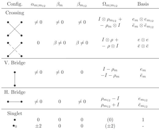
4.1.1 Crossing and bridge pairs of standard Young tableaux . . . 56

4.1.2 Islands . . . 57

4.1.3 Reduced subduction graph . . . 63

4.2 A higher dimension example: the first multiplicity-three case . . . 63

5 The subduction problem for Brauer algebras 67 5.1 Irreducible representations of Brauer algebras . . . 68

5.1.1 Generalized tableaux . . . 68

5.1.2 Permutation lattices . . . 70

5.1.3 Labelling for the Gelfand-Tzetlin base . . . 71

5.1.4 Transpose permutation lattice . . . 72

5.1.5 Some combinatoric functions for permutation lattices . . . 73

5.1.6 Explicit actions . . . 74

5.2 The subduction problem . . . 76

5.2.1 Subduction system . . . 77

5.2.2 Explicit form of the subduction system . . . 78

5.3 Subduction graph . . . 83

5.4 Structure of the subduction space . . . 84

5.4.1 Crossing space . . . 84

5.4.2 Bridge spaces . . . 85

5.4.3 Singlet space . . . 86

5.5 Orthonormalization and phase conventions . . . 87

Representation theory of classical Lie groups (unitary, orthogonal and symplec-tic groups) plays a fundamental role in many areas of physics and chemistry. Orthogonal and symplectic group representation theory arises, for example, in the description of sym-metrized orbitals in quantum chemistry and in fermion and boson many-body theory [1], grand unification theories for elementary particles [2], supergravity [3], interacting boson and fermion dynamical symmetry models for nuclei [4, 5], nuclear symplectic models [6, 7], and so on.

In particular, the importance of coupling and recoupling coefficients (Clebsch-Gordan coefficients, 6j-symbols, Racah coefficients, 9j-symbols and general 3nj-symbols) is evident in the study of angular momentum theory which is built on the well known representation theory of SU (2). Furthermore, Racah-Wigner calculus of SU (2) group has notable applications in the theory of orthogonal polynomials and other special functions.

The Racah coefficients and other recoupling coefficients of unitary SU (n), orthogo-nal SO(n) and symplectic Sp(2m) groups of different rank are quite useful when calculating energy levels and transition rates in atomic, molecular and nuclear theory (for example, in connection with the Jahn-Teller effect and structural analysis of atomic shells, see Judd and co-workers [8, 9] and, for a description of multi-bosonic and multi-fermionic systems and applications in the microscopic nuclear theory, consider [10, 11]), and in conformal field theory [12].

There are many approaches to the Racah coefficients, but the problem is that there are no general methods for treating various kind of coupling and recoupling issues. Any given technique applies only to a particular problem and for a particular group. Not only

do the tecniques for dealing with unitary, orthogonal and symplectic groups all drastically differ from each other, but the methods for finding the various Wigner coefficients, which we are interested in, also vary from one to the other. Furthermore, analytical expressions are difficult to come by for general Lie groups, mainly because there is a multiplicity problem in the reduction of Kronecker products of pair of irreducible representations. Some missing labels need to be added in, for which a procedure is often difficult to do systematically. Finally, although several efficient computer codes and numerical procedures exist, they often do not permit any insight in the mathematical structure of such coefficients and, however, a general and efficient closed algorithm is still needed. Therefore, citing Jin-Quan Chen in his book Group representation theory for physicists, “in many cases, these methods are more of an art than a science”.

The aim of this thesis is to provide a systematic and comprehensive approach to deal with the structure of coupling coefficients for classical Lie groups. The most promising strategy, from this point of view, seems to be the one building on the well-known and tight connection between symmetric and unitary groups which is called in literature

Schur-Weyl duality and which was first pointed out by Schur at the beginning of the twentieth

century [13]. Schur proved that the image of each group under its representation equals the full centralizer algebra and that the two actions are omeomorphic. This observation was developed ten years later by Brauer [14] who found the full centralizer algebra for orthogonal and symplectic groups and completed the construction of the full centralizer algebras for the classical series of the Lie groups.

Weyl used these results, gave numerous theorems concerned with irreducible repre-sentations of both classical Lie group and its centralizer algebras, and also gave application to the many-body sistems of f equivalent particles. However, the duality goes further than the one originally expressed by Schur and Weyl. Many powerful equalities between various tranformation factors of the centralizer algebras and those of the corresponding Lie group can be established. This is one of the main aims of the invariant theory.

different symmetric group chains (so called Gelfand-Tzetlin chains) to define his f symbol (our subduction factor) for a symmetric group. He showed that the f symbols were equiv-alent to recoupling coefficients (6j and 9j symbols) for any unitary group and further that

f symbols were also equal to coupling coefficients for U (p + q) ⊃ U (p) × U (q). Later [16]

such results were generalized to Brauer centralizer algebras and to the corresponding ortho-symplectic groups, making the problem of finding coupling and recoupling coefficients for classical Lie groups equivalent to the subduction problem for centralizer algebras.

Subduction coefficients for symmetric groups were first introduced in 1953 by Elliot

et al to describe the states of a physical system with n identical particles as composed

of two subsystems with n1 and n2 particles respectively (n1 + n2 = n) and then they

were soon generalized to Brauer algebras [17]. Since Elliot’s work, many techniques have been proposed for calculating the subduction coefficients, but the investigation is until now incomplete. The main goal to give explicit and general closed algebraic formulas has not been achieved. Only some special cases have been solved for symmetric groups. There are also numerical methods which are used to approach the issue, but, again as in the case of recoupling coefficients, no insight into the structure of the trasformation coefficients can be obtained. Another outstanding problem is the resolution of multiplicity separations in a systematic manner, indicating a consistent choice of the indipendent phases and free factors. In this thesis, we choose an algebraic approach to the subduction problem in sym-metric groups Sn ↓ Sn1 × Sn2 and in Brauer algebras Bf(x) ↓ Bf1(x) × Bf2(x) and we

analyze in detail the linear equation method [18], an efficient tool for deriving algebraic solu-tions for fixed values of n1, n2 and f1, f2respectively. Thus we give a suitable combinatorial

description of the equation system arisen from the method and we provide a new algorithm to solve it. Therefore, by solving the subduction problem for centralizer algebras, we have the solution for a unified approach to the Racah-Wigner calculus for classical Lie groups.

There are at least three possible interesting developments for this thesis: • Racah-Wigner calculus for quantized enveloping algebras.

quan-tized enveloping algebras are well characterized both from the algebraic and combi-natorial point of view and there exists an explicit construction of their irreducible representations [19]. Thus, the linear equation method can be directly applied to this issue without any particular difficulty.

• Racah-Wigner calculus for projective representations of classical Lie groups.

Projective (spinor) representations of a classical Lie group G are very useful in many situations. Finding such representations is equivalent to determining the tensorial irreducible representations of the universal enveloping group of G (which is another classical Lie group). An alternative approach is to find the projective representations of Brauer algebras. The Gelfand-Tzetlin basis for such representations is described in terms of combinatorial objects which are known as stable-up-down tableaux [20] (they are permutation lattices with null elements, in our language). Unfortunately, the explicit action on the irreducible invariant spaces is still unknown.

• Racah-Wigner calculus for exceptional Lie groups

Racah-Wigner calculus for exceptional Lie groups also has many applications both in physics and mathematical physics. The study of the subduction problem for this case would be important for a comprehensive knowledge of Racah-Wigner calculus for all Lie groups. The centralizer algebras for exceptional Lie groups are still unknown.

The layout of the thesis is the following.

In chapter 1, we review some basic results in representation theory of classical Lie groups which are necessary to deal with the coupling and recoupling problem. We mainly consider the construction of standard Gelfand-Tzetlin bases and the explicit action of classical Lie algebras on such bases.

The definitions of classical coupling and recoupling coefficients for the groups

SU (2) and SO(3) are also given and then generalized to generic classical Lie groups.

Be-sides classical duality, a description of quantum deformation groups and the corresponding centralizer algebras is given.

After that, we specialize the discussion on the Bf(²n) − SO(n)/Sp(2n) duality

and we highlight the relation between subduction and Racah coefficients.

In chapter 3, we investigate the linear equation method for symmetric groups, proposed by Chen et al. for the determination of the subduction coefficients as solution of a linear system. We prove that such a system, which is constituted by a complicated primal structure of dependent linear equations, can be simplified by choosing a minimal set of sufficient equations related to the concept of subduction graph. Furthermore, the subduction graph provides a very practical way to choose such equations and it suggests that subduction coefficients may be seen as a subspace of Rfλ

⊗ Rfλ1fλ2 _{(where f}λ_{, f}λ1_{, f}λ2 _are

the dimensions of the irreducible representations involved in the subduction Sn↓ Sn1×Sn2)

obtained by the intersection of only n − 2 explicit subspaces (each one in corrispondence with an i-layer) instead of the original (n − 2)fλ_fλ1_fλ2 _{ones. Consequently, we have a more}

explicit insight into the structure of the transformation from the standard basis to the split basis.

Furthermore, we propose a general form for the subduction coefficients resulting from the only requirement of orthonormality and we note that the multiplicity separation can be described in terms of the Sylvester matrix of the positive defined quadratic form τ describing the scalar product in the subduction space. Thus we are able to link the freedom to fix the multiplicity separation to the freedom to choose of the Sylvester matrix. The number of phases and free factors of the general multiplicity separation can be expressed as functions of the multiplicity µ (i.e. the dimension of the subduction space). A crucial question is the possibility to fix the Sylvester matrix to obtain all the requirements of

simplicity given in [21] for the form of each coefficient. We conjecture that such a form only

depends on the form of the eigenvalues and eigenvectors of τ . (These results are published in [22].)

of the symmetric group Sn. A selection rule which allows to determine the vanishing

sub-duction coefficients and to organize the other ones in blocks (named islands) is given. We prove that all islands produce the same values for the subduction coefficients and thus only a much smaller number of them really needs to be evaluated. Thus, the linear equa-tion method, described in terms of a reduced subducequa-tion graph, provides a systematic and optimizated tool to calculate the unknown transformation coefficients.

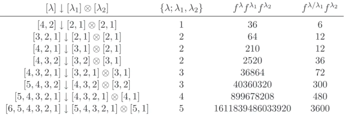
As a significative example, the first multiplicity-three cases, [4, 3, 2, 1] ↓ [3, 2, 1] ⊗ [3, 1] and its conjugate [4, 3, 2, 1] ↓ [3, 2, 1] ⊗ [2, 1, 1] for S10↓ S6× S4, were dealt in detail:

we give the suitable orthonormalized transformation coefficients relative to each multiplicity copy descending from the Yamanouchi phase convention.

(These results are published in [23])

Finally, in chapter 5, we describe the subduction problem for Brauer algebras. This problem is clearly a generalization of the corresponding one for symmetric groups be-cause the group algebra CSf is strictly included in Bf(x). After the suitable combinatorial

description for the Gelfand-Tzetlin basis by the introduction of Bratteli diagrams and

per-mutation lattices (which generalize the concept of standard Young tableau), we provide the

explicit action of Brauer algebra generators on the irreducible invariant spaces. This allows us to write the explicit form of the subduction equations deriving from the linear method. A description of the solution of such equations is given trhough the concept of a generalized i-layer. We find four possible configurations for the subduction space and we can provide a definition of subduction graph analogous to that one given in chapter 3.

Finally, as in chapter 3, the form for the orthonormalized subduction coefficients is discussed with a special emphasis on the choice of Young-Yamanouchi phase and the other free factors.

(These results are in preparation to be submitted for publication.)

I wish to thank Massimo Campostrini for introducing me into this interesting research topic and for his valuable support during the progress of this thesis.

Classical Lie algebras, classical Lie

groups and Racah-Wigner calculus

This chapter is devoted to a rapid review of Racah-Wigner calculus for classical Lie groups and the envolved representation theory. In section 1, we deal with Gelfand-Tzetlin bases and explicit actions of Lie groups and algebras on such bases. In section 2, the basic results of Racah-Wigner calculus for SU (2) group are presented and, in section 3, they are generalized to classical Lie groups.

1.1

Bases and operators

The simple Lie algebras over the field of complex numbers were classified in the works of Cartan and Killing in the 1930’s. There are four infinite series A_n, B_n, C_n, D_n which are called the classical Lie algebras, and five exceptional Lie algebras E6, E7, E8, F4,

G₂. The structure of these Lie algebras is uniformly described in terms of certain finite sets of vectors in a Euclidean space called the root systems. Due to Weyl’s complete reducibility theorem, the theory of finite-dimensional representations of the semisimple Lie algebras is largely reduced to the study of irreducible representations.

The irreducible representations are parametrized by their highest weights. The characters and dimensions are explicitly known by the Weyl formula. The reader is

ered to, e.g., the books of Bourbaki [24], Dixmier [25], Humphreys [26] or Goodman and Wallach [27] for a detailed exposition of the theory.

However, the Weyl formula for the dimension does not use any explicit construction of the representations. Such constructions remained unknown until 1950 when Gelfand and Tzetlin1published two short papers [28] and [29] (in Russian) where they solved the problem for the general linear Lie algebras (type An) and the orthogonal Lie algebras (types Bn and

D_n), respectively. Baird and Biedenharn employed the calculus of Young patterns to derive the Gelfand-Tzetlin formulas. Their interest to the formulas was also motivated by the connection with the fundamental Wigner coefficients.

A year earlier (1962) Zhelobenko published an independent work [30] where he derived the branching rules for all classical Lie algebras. In his approach the representa-tions are realized in a space of polynomials satisfying the “indicator system” of differential equations. He outlined a method to construct the lowering operators and to derive the matrix element formulas for the case of the general linear Lie algebra gl_n. An explicit “infinitesimal” form for the lowering operators as elements of the enveloping algebra was found by Nagel and Moshinsky [31] (1964) and independently by Hou Pei-yu [32] (1966). The latter work relies on Zhelobenko’s results [30] and also contains a derivation of the Gelfand-Tzetlin formulas alternative to that of Baird and Biedenharn. This approach was further developed in the book by Zhelobenko [33] which contains its detailed account.

The work of Nagel and Moshinsky was extended to the orthogonal Lie algebras oN

by Pang and Hecht [34] and Wong [35] who produced explicit infinitesimal expressions for the lowering operators and gave a derivation of the formulas of Gelfand and Tzetlin [29].

During the half a century passed since the work of Gelfand and Tsetlin, many different approaches were developed to construct bases of the representations of the classical Lie algebras. New interpretations of the lowering operators and new proofs of the Gelfand-Tzetlin formulas were discovered by several authors. In particular, Gould [36, 37, 38, 39] employed the characteristic identities of Bracken and Green [40, 41] to calculate the

Wigner coefficients and matrix elements of generators of gl_nand o_N. The extremal projector discovered by Asherova, Smirnov and Tolstoy [42, 43, 44] turned out to be a powerful

instrument in the representation theory of the simple Lie algebras. It plays an essential role in the theory of Mickelsson algebras developed by Zhelobenko which has a wide spectrum of applications from the branching rules and reduction problems to the classification of Harish-Chandra invarian irreducible spaces; see Zhelobenko’s expository paper [45] and his book [46]. Two different quantum minor interpretations of the lowering and raising operators were given by Nazarov and Tarasov [47] and the author [48]. These techniques are based on the theory of quantum algebras called the Yangians and allow an independent derivation of the matrix element formulas.

1.1.1 Gelfand-Tzetlin basis

We now discuss the main idea which leads to the construction of the Gelfand-Tzetlin bases. The first point is to regard a given classical Lie algebra not as a single object but as a part of a chain of subalgebras with natural embeddings. We illustrate this idea using representations of the symmetric groups Sn as an example. Consider the chain of

subgroups

S1 ⊂ S2⊂ · · · ⊂ Sn, (1.1)

where the subgroup Skof Sk+1consists of the permutations of the set {1, 2, . . . , k +1} with

the index k + 1. The irreducible representations of the group Sn are indexed by partitions

λ of n. A partition λ = (λ1, . . . , λl) with λ1 ≥ λ2 ≥ · · · ≥ λl is depicted graphically as a

Young diagram which consists of l left-justified rows of boxes so that the top row contains λ1 boxes, the second row λ2 boxes, etc. Denote by V (λ) the irreducible representation of

Sncorresponding to the partition λ. One of the central results of the representation theory

of the symmetric groups is the following branching rule which describes the restriction of

V (λ) to the subgroup Sn−1:

V (λ)|_Sn−1 = ⊕

µV

0_{(µ), (1.2)}

summed over all partitions µ whose Young diagram is obtained from that of λ by removing one box. Here V0_{(µ) denotes the irreducible representation of S}

n−1 corresponding to a

partition µ. Thus, the restriction of V (λ) to Sn−1 is multiplicity-free, i.e., is contains

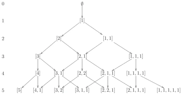
natural parameterization of the basis vectors in V (λ) by taking its further restrictions to the subsequent subgroups of the chain (1.1). Namely, the basis vectors will be parametrized by sequences of partitions

λ(1) → λ(2) → · · · → λ(n)= λ, (1.3)

where λ(k) _{is obtained from λ}(k+1) _{by removing one box. Equivalently, each sequence of}

this type can be regarded as a standard tableau of shape λ which is obtained by writing the numbers 1, . . . , n into the boxes of λ in such a way that the numbers increase along the rows and down the columns. In particular, the dimension of V (λ) equals the number of standard tableaux of shape λ. There is only one irreducible representation of the trivial group S1

therefore the procedure defines basis vectors up to a scalar factor. The corresponding basis is called the Young basis. The symmetric group Snis generated by the adjacent transpositions

gi = (i, i + 1). The construction of the representation V (λ) can be completed by deriving

explicit formulas for the action of the elements giin the basis which are also due to A. Young.

This realization of V (λ) is usually called Young’s orthogonal (or seminormal) form. The details can be found, e.g., in James and Kerber [49] and Sagan [50]; see also Okounkov and Vershik [51] where an alternative construction of the Young basis is produced.

Quite a similar method can be applied to representations of the classical Lie alge-bras. Consider the general linear Lie algebra gl_n which consists of complex n × n-matrices with the usual matrix commutator. The chain (1.1) is now replaced by

gl₁⊂ gl₂ ⊂ · · · ⊂ gl_n, (1.4)

with natural embeddings gl_k ⊂ gl_k+1. The orthogonal Lie algebra oN can be regarded as

a subalgebra of gl_N which consists of skew-symmetric matrices. Again, we have a natural chain

o2 ⊂ o3 ⊂ · · · ⊂ oN. (1.5)

Both restrictions gl_n↓ gl_n−1 and o_N ↓ o_{N −1} are multiplicity-free so that the application of the argument which we used for the chain (1.1) produces basis vectors in an irreducible rep-resentation of gl_nor oN. With an appropriate normalization, these bases are precisely those

vectors here are parametrized by combinatorial objects called the Gelfand-Tzetlin patterns. However, this approach does not work for the symplectic Lie algebras sp_2n since the re-striction sp_2n↓ sp_2n−2 is not multiplicity-free. The multiplicities are given by Zhelobenko’s branching rule [30] which was re-discovered later by Hegerfeldt [52]. Various approaches to fix this problem were made by several authors [53, 54, 55, 56, 57].

1.1.2 Explicit operatorial construction for gl_n

Now, we give some classical results of representation theory with special regard to the construction of the action of the algebra generators on irreducible invariant spaces.

Let Eij, i, j = 1, . . . , n denote the standard basis of the general linear Lie algebra

gl_nover the field of complex numbers. The subalgebra gl_n−1is spanned by the basis elements

Eij with i, j = 1, . . . , n − 1. Denote by h = hn the diagonal Cartan subalgebra in gln. The

elements E11, . . . , Enn form a basis of h. Finite-dimensional irreducible representations of

gl_n are in a one-to-one correspondence with n-tuples of complex numbers λ = (λ1, . . . , λn)

such that

λi− λi+1∈ Z+ for i = 1, . . . , n − 1. (1.6)

Such an n-tuple λ is called the highest weight of the corresponding representation which we shall denote by L(λ). It contains a unique, up to a multiple, nonzero vector ξ (the highest

vector ) such that Eiiξ = λiξ for i = 1, . . . , n and Eijξ = 0 for 1 ≤ i < j ≤ n.

The following theorem is the branching rule for the reduction gl_n↓ gl_n−1.

Theorem 1.1.1. The restriction of L(λ) to the subalgebra gl_n−1 is isomorphic to the direct sum of pairwise inequivalent irreducible representations

L(λ)|_gl

n−1 ' ⊕_µL

0_{(µ), (1.7)}

summed over the highest weights µ satisfying the betweenness conditions

λi− µi ∈ Z+ and µi− λi+1∈ Z+ for i = 1, . . . , n − 1. (1.8)

The rule could presumably be attributed to I. Schur who was the first to dis-cover the representation-theoretic significance of a particular class of symmetric polynomi-als which now bear his name. The subsequent applications of the branching rule to the

subalgebras of the chain

gl₁ ⊂ gl₂ ⊂ · · · ⊂ gl_n−1⊂ gl_n (1.9)

yield a parameterization of basis vectors in L(λ) by the combinatorial objects called the

Gelfand-Tzetlin patterns. Such a pattern Λ (associated with λ) is an array of row vectors

λ_n1 λ_n2 · · · λ_nn

λ_n−1,1 · · · λ_n−1,n−1 · · · · · · · · ·

λ₂₁ λ₂₂ λ₁₁

where the upper row coincides with λ and the following conditions hold

λ_ki− λ_k−1,i ∈ Z+, λk−1,i− λk,i+1 ∈ Z+, i = 1, . . . , k − 1 (1.10)

for each k = 2, . . . , n. The Gelfand-Tzetlin basis of L(λ) is provided by the following theorem. Let us set l_ki= λ_ki− i + 1.

Theorem 1.1.2. There exists a basis {ξ_Λ} in L(λ) parametrized by all patterns Λ such that the action of generators of gl_n is given by the formulas

E_kkξ_Λ= Ã k X i=1 λ_ki− k−1 X i=1 λ_k−1,i ! ξ_Λ, (1.11) Ek,k+1ξΛ= − k X i=1 (l_ki− l_k+1,1) · · · (l_ki− l_k+1,k+1) (l_ki− l_k1) · · · ∧ · · · (l_ki− l_kk) ξΛ+δki, (1.12) Ek+1,kξΛ= k X i=1 (l_ki− l_k−1,1) · · · (l_ki− l_k−1,k−1) (l_ki− l_k1) · · · ∧ · · · (l_ki− l_kk) ξΛ−δki. (1.13)

The arrays Λ ± δ_ki are obtained from Λ by replacing λ_ki by λ_ki ± 1. It is supposed that ξ_Λ = 0 if the array Λ is not a pattern; the symbol ∧ indicates that the zero factor in the

denominator is skipped.

The vector space L(λ) is equipped with a contravariant inner product h , i. It is uniquely determined by the conditions

for any vectors η, ζ ∈ L(λ) and any indices i, j. In other words, for the adjoint operator for

Eij with respect to the inner product we have (Eij)∗= Eji.

Proposition 1.1.3. The basis {ξ_Λ} is orthogonal with respect to the inner product h , i. Moreover, we have h ξ_Λ, ξ_Λi = n Y k=2 Y 1≤i≤j<k (lki− lk−1,j)! (lk−1,i− lk−1,j)! Y 1≤i<j≤k (lki− lkj− 1)! (lk−1,i− lkj − 1)! . (1.15)

The formulas of Theorem 1.1.2 can therefore be rewritten in the orthonormal basis

ζ_Λ = ξ_Λ/k ξ_Λk, k ξ_Λk2 = h ξ_Λ, ξ_Λi. (1.16) 1.1.3 Gelfand-Tzetlin bases for the other classical Lie algebras

Let gn denote the rank n simple complex Lie algebra of type B, C, or D. That is,

gn= o2n+1, sp2n, or o2n, (1.17)

respectively. Let V (λ) denote the finite-dimensional irreducible representation of gn with

the highest weight λ. The restriction of V (λ) to the subalgebra gn−1is not multiplicity-free

in general. This means that if V0_{(µ) is the finite-dimensional irreducible representation of}

gn−1 with the highest weight µ, then the space

Homg_n−1(V0(µ), V (λ)) (1.18)

need not be one-dimensional. In order to construct a basis of V (λ) associated with the chain of subalgebras

g1 ⊂ g2 ⊂ · · · ⊂ gn (1.19)

we need to construct a basis of the space (1.18) which is isomorphic to the subspace V (λ)+

µ

of gl_n−1-highest vectors of weight µ in V (λ). The restriction of V (λ) to the subalgebra gn−1

is given by

V (λ)|_gn−1 ' ⊕

µc(µ) V

0_{(µ), (1.20)}

where V0_{(µ) is the irreducible finite-dimensional representation of g}

n−1 with the highest

exact value is found from the Zhelobenko branching rules [30]. In the formulas below we use the notation

li = λi+ ρi+ 1/2, γi = νi+ ρi+ 1/2, (1.21)

where the νi are the parameters defined in the branching rules. A parameterization of basis

vectors in V (λ) is obtained by applying the branching rules to its subsequent restrictions to the subalgebras of the chain

g1⊂ g2⊂ · · · ⊂ gn−1⊂ gn. (1.22)

This leads to the definition of the Gelfand-Tzetlin patterns for the B, C and D types. Then we give formulas for the basis vectors of the representation V (λ). We use the notation

lki = λki+ ρi+ 1/2, l0ki= λ0ki+ ρi+ 1/2, (1.23)

where the λki and λ0_ki are the entries of the patterns defined below.

B type case. The multiplicity c(µ) equals the number of n-tuples (ν0

1, ν2, . . . , νn) satisfying the inequalities − λ₁ ≥ ν₁0 ≥ λ₁≥ ν₂≥ λ₂ ≥ · · · ≥ ν_n−1≥ λ_n−1≥ ν_n≥ λ_n, − µ₁ ≥ ν₁0 ≥ µ₁ ≥ ν₂ ≥ µ₂ ≥ · · · ≥ ν_n−1≥ µ_n−1≥ ν_n (1.24) with ν0

1 and all the νi being simultaneously integers or half-integers together with the λi.

Equivalently, c(µ) equals the number of (n + 1)-tuples ν = (σ, ν1, . . . , νn), with the entries

given by (σ, ν1) =      (0, ν0 1) if ν10≤ 0, (1, −ν0 1) if ν10> 0. (1.25)

Lemma 1.1.4. The vectors

ξν = zn0σ n−1_Y i=1 zνi−µi ni zi,−nνi−λi· γ_Yn−1 k=ln Zn,−n(k) ξ (1.26)

form a basis of the space V (λ)+

Define the B type pattern Λ associated with λ as an array of the form σ_n λ_n1 λ_n2 · · · λ_nn λ0_n1 λ0_n2 · · · λ0_nn σ_n−1 λ_n−1,1 · · · λ_n−1,n−1 λ0_n−1,1 · · · λ0_n−1,n−1 · · · · · · · · · σ₁ λ₁₁ λ0₁₁

such that λ = (λ_n1, . . . , λ_nn), each σ_k is 0 or 1, the remaining entries are all non-positive integers or non-positive half-integers together with the λi, and the following inequalities

hold

λ0_k1≥ λ_k1≥ λ0_k2 ≥ λ_k2≥ · · · ≥ λ0_k,k−1≥ λ_k,k−1≥ λ0_kk ≥ λ_kk (1.27) for k = 1, . . . , n, and

λ0_k1≥ λ_k−1,1≥ λ0_k2 ≥ λ_k−1,2≥ · · · ≥ λ0_k,k−1≥ λ_k−1,k−1 ≥ λ0_kk (1.28) for k = 2, . . . , n. In addition, in the case of the integer λ_i the condition

λ0_k1≤ −1 if σ_k = 1 (1.29)

should hold for all k = 1, . . . , n.

Theorem 1.1.5. The vectors

ξ_Λ= → Y k=1,...,n  zσk k0 · k−1_Y i=1 zλ0ki−λk−1,i ki z λ0 ki−λki i,−k · l0 kkY−1 j=l_kk Zk,−k(j)   ξ (1.30)

parametrized by the patterns Λ form a basis of the representation V (λ).

C type case. The multiplicity c(µ) equals the number of n-tuples of integers (ν₁, . . . , ν_n) satisfying the inequalities

0 ≥ ν1≥ λ1 ≥ ν2 ≥ λ2≥ · · · ≥ νn−1≥ λn−1≥ νn≥ λn,

0 ≥ ν1≥ µ1≥ ν2≥ µ2 ≥ · · · ≥ νn−1≥ µn−1≥ νn.

Lemma 1.1.6. The vectors ξν = n−1_Y i=1 zνi−µi ni zi,−nνi−λi · γ_Yn−1 k=ln Zn,−n(k) ξ (1.32)

form a basis of the space V (λ)+_µ.

Define the C type pattern Λ associated with λ as an array of the form

λ_n1 λ_n2 · · · λ_nn λ0_n1 λ0_n2 · · · λ0_nn λ_n−1,1 · · · λ_n−1,n−1 λ0_n−1,1 · · · λ0_n−1,n−1 · · · · · · λ₁₁ λ0₁₁

such that λ = (λ_n1, . . . , λ_nn), the remaining entries are all non-positive integers and the following inequalities hold

0 ≥ λ0_k1≥ λ_k1≥ λ0_k2 ≥ λ_k2≥ · · · ≥ λ0_k,k−1≥ λ_k,k−1≥ λ0_kk ≥ λ_kk (1.33)

for k = 1, . . . , n, and

0 ≥ λ0_k1≥ λ_k−1,1≥ λ0_k2 ≥ λ_k−1,2≥ · · · ≥ λ0_k,k−1≥ λ_k−1,k−1 ≥ λ0_kk (1.34)

for k = 2, . . . , n.

Theorem 1.1.7. The vectors

ξ_Λ= → Y k=1,...,n  k−1Y i=1 zλ 0 ki−λk−1,i ki z λ0 ki−λki i,−k · l0 kkY−1 j=l_kk Zk,−k(j)   ξ (1.35)

D type case. The multiplicity c(µ) equals the number of (n − 1)-tuples (ν1, . . . , νn−1)

satisfying the inequalities

−|λ1| ≥ ν1 ≥ λ2≥ ν2≥ λ3 ≥ · · · ≥ λn−1≥ νn−1≥ λn,

−|µ1| ≥ ν1 ≥ µ2 ≥ ν2 ≥ µ3≥ · · · ≥ µn−1 ≥ νn−1

(1.36) with all the νi being simultaneously integers or half-integers together with the λi. Set

ν0 = max{λ1, µ1}.

Lemma 1.1.8. The vectors ξ_ν = n−1_Y i=1 zνi−1−µi ni z νi−1−λi i,−n · γn−1_Y−2 k=ln Z_n,−n(k) ξ (1.37)

form a basis of the space V (λ)+

µ.

Define the D type pattern Λ associated with λ as an array of the form

λ_n1 λ_n2 · · · λ_nn λ0_n−1,1 · · · λ0_n−1,n−1 λ_n−1,1 · · · λ_n−1,n−1 · · · · · · λ₂₁ λ₂₂ λ0₁₁ λ₁₁

such that λ = (λ_n1, . . . , λ_nn), the remaining entries are all positive integers or non-positive half-integers together with the λ_i, and the following inequalities hold

−|λ_k1| ≥ λ0_k−1,1≥ λ_k2≥ λ_k−1,20 ≥ · · · ≥ λ_k,k−1≥ λ0_k−1,k−1≥ λ_kk, (1.38)

−|λ_k−1,1| ≥ λ0_k−1,1≥ λ_k−1,2≥ λ0_k−1,2≥ · · · ≥ λ_k−1,k−1≥ λ0_k−1,k−1 (1.39) for k = 2, . . . , n. Set λ0

k−1,0= max{λk1, λk−1,1}. Theorem 1.1.9. The vectors

ξ_Λ= → Y k=2,...,n  k−1Y i=1 zλ 0 k−1,i−1−λk−1,i ki z λ0 k−1,i−1−λki i,−k · l0 k−1,k−1_Y−2 j=l_kk Zk,−k(j)   ξ (1.40)

1.2

Coupling and recoupling for the SO(3) group

1.2.1 Clebsch-Gordan coefficients

Clebsch-Gordan coefficients (CGCs) usually refer to the group SO(3) and are used

in physics to integrate products of three spherical harmonics. They arise in applications involving the addition of angular momentum in quantum mechanics [58]. The CGCs are var-iously written as Cmj1m2, C

j1j2j

m1m2m, (j1, j2; m1, m2|j1, j2; j, m), or hj1, j2; m1, m2|j1, j2; j, mi.

Equivalently, they are used in the representation theory of SU (2) and SO(3) groups to perform the explicit direct sum decomposition of the tensor product of two irreducible representations into irreducible representations, in cases where the numbers and types of irreducible components are already known. The name derives from the German mathe-maticians Alfred Clebsch (1833-1872) and Paul Gordan (1837-1912), who encountered an equivalent problem in invariant theory.

From the previous subsection, we know that the irreducible representations for the

A₁ algebra (the Lie algebra associated to the grop SU (2)) are labelled by a nonnegative half-integer number (associated with the Gelfand-Tzetlin pattern) that we may denote by

j and their dimension is given by 2j + 1. Because SU (2) is the covering group of SO(3), j labels an irreducible representation (irrep) of SO(3) if j is an integer (so-called tensorial

irreps) and a projective one if j is not an integer (so-called spinor irreps).

Given the tensor product representation j1⊗ j2 for SU (2), it is an outstanding

question which irreps are contained in its decomposition in direct sum of invariant irre-ducible spaces. In fact, such a decomposition has the important physical meaning of the sum of two angular momenta j1 and j2 respectively. By definition, CGCs are the entries of

the orthogonal base changing matrix which reduces j1⊗j2in a block diagonal form. Because

such a decomposition is multiplicity-free, denoted by |j, mi (m ∈ {−j, −j + 1, . . . , j − 1, j}) a generic Gelfand-Tzetlin base vector for j and by |j1, m1i and |j2, m2i for j1 and j2

respec-tively, we have |j1, j2; j, mi = j1 X m1=−j1 j2 X m2=−j2 |j1, j2; m1, m2ihj1, j2; m1, m2|j1, j2; j, mi (1.41)

orthonormalized and defining the suitable raising and lowering operetors as described in the previous section, we obtain the following relation for the CGCs:

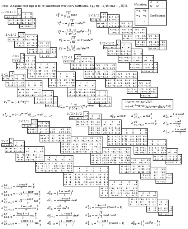
p (j ∓ m + 1)(j ± m) hj1, j2; m1, m2|j1, j2; j, mi = p (j₁∓ m₁+ 1)(j₁± m₁) hj₁, j₂; m₁∓ 1, m₂|j₁, j₂; j, m ∓ 1i + p (j₂∓ m₂+ 1)(j₂± m₂) hj₁, j₂; m₁, m₂∓ 1|j₁, j₂; j, m ∓ 1i (1.42) which is often useful for finding the last CGCs, when the other one or two coefficients in the formula are known. Note that there are sometimes only two coefficients in that equation, the third being both invalid (j < |m|) and multiplied by 0. Furthermore (1.42) provides a recursion relation that can be useful for finding the explicit expression of the coefficients. In figure 1.1 a well-known table with the values of CGCs for several coupling irreps is given.

CGCs are sometimes associated to the so-called 3j-symbols (or Wigner

coeffi-cients), denoted by _

 j1 j2 J

m₁ m₂ M

 

where, as usual, the entries of the symbol j1, j2, J, m1, m2 and M are either integer or

half-integer [59]. 3j − symbols satisfy the following selection rules:

1. m1 ∈ {−|j1|, ..., |j1|}, m2 ∈ {−|j2|, ..., |j2|}, and M ∈ {−|J|, ..., |J|}.

2. m1+ m2= M .

3. Triangular inequalities: |j1− j2| ≤ J ≤ j1+ j2.

4. Integer perimeter rule: j1+ j2+ J is an integer.

Note that not all these rules are independent, since rule (4) is implied by the other three. If these conditions are not satisfied the 3j-symbol vanishes.

Figure 1.1: Clebsch-Gordan coefficients for several coupling (tensorial and projective) ir-reps of SO(3). The sign convention is that of Wigner [60], also used by Con-don and Shortley [61], Rose [62], and Cohen [63]. The coefficients here have been calculated using computer programs written independently by Cohen et al. at LBNL.

Furthermore, the Wigner 3j-symbols have the symmetries:   j1 j2 J m1 m2 M   =   j2 J j1 m2 M m1   _(1.43) =   J j1 j2 M m1 m2   _(1.44) = (−1)j1+j2+J   j2 j1 J m2 m1 M   _(1.45) = (−1)j1+j2+J   j1 J j2 m₁ M m₂   _(1.46) = (−1)j1+j2+J   J j2 j1 M m₂ m₁   _(1.47) = (−1)j1+j2+J   j1 j2 J −m1 −m2 −M   _(1.48)

and they obey the orthogonality relations X j,m (2j + 1)   j1 j2 J m1 m2 M     j1 j2 J m0 1 m02 M   = δ_m1,m0 1δm2,m02 (1.49) X m1,m2 (2j + 1)   j1 j2 J m1 m2 M     j1 j2 J0 m0 1 m02 M0   = δJ,J0δ_M,M0. (1.50)

The connection between 3j-symbols and Clebsch-Gordan coeficients is given by the relation:

hj₁j₂; m₁m₂|j₁j₂; jmi = (−1)m+j1−j2p_{2j + 1}   j1 j2 j m1 m2 −m   . (1.51)

1.2.2 Racah coefficients and general recoupling symbols

Racah coefficients U (j1j2jj3; j12j23) (sometimes called U coefficients) represent

the elements of a unitary matrix between bases with two different coupling orders of three irreps j1, j2 an j3:

|(j₁j₂)j₁₂, j₃; jj0i =X

j23

The U coefficients satisfy the following unitay conditions X j23 U (j1j2jj3; j12j23) U (j1j2jj3; ¯j12j23) = δj12¯j12 (1.53) X j12 U (j1j2jj3; j12j23) U (j1j2jj3; j12¯j23) = δj23¯j23 (1.54)

deriving from the fact that we deal with orthonormalized bases.

Sometimes one needs to use 6j −symbols which is defined in terms of U coefficients

by [64] _   j1 j2 j12 j3 j j23   = 1 p (2j12+ 1)(2j23+ 1) U (j1j2jj3; j12j23) (1.55)

Thus, the 6j-symbols are defined for integers and half-integers j₁, j₂, j₁₂, j₃, j, j₂₃ whose triads (j1, j2, j12), (j1, j, j23), (j3, j2, j23), and (j3, j, j12) satisfy the following conditions

1. Each triad satisfies the triangular inequalities.

2. The sum of the elements of each triad is an integer. Therefore, the members of each triad are either all integers or contain two half-integers and one integer.

If these conditions are not satisfied, the 6j-symbol vanishes.

Suppose we have a tetrahedron, labelled so that the three labels around each face satisfy the conditions given above, thus we have a so-called an admissible labelling. This tetrahedral picture is traditionally used to simply express the symmetry of the 6j-symbol, which is naturally invariant under the full tetrahedral group S4. In particular, they are

invariant [65] under permutation of their columns, e.g.,    j1 j2 j12 j3 j j23   =    j2 j1 j12 j j3 j23    (1.56)

and under exchange of two corresponding elements between rows, e.g.    j1 j2 j12 j3 j j23   =    j3 j j12 j1 j2 j23   . (1.57)

The following Racah-Elliot and orthogonality relations are often useful for com-puting numerical values or exact expressions:

X j12 (−1)2j12_(2j 12+ 1)    j1 j2 j12 j₁ j₂ j₂₃   = 1 (1.58) X j12 (−1)j1+j2+j12 _(2j 12+ 1)    j1 j2 j12 j2 j1 j23   = δj1j23 p (2ji+ 1)(2j2+ 1) (1.59) X j12 (2j12+ 1)    j1 j2 j12 j₃ j j₂₃       j3 j j12 j₁ j₂ ¯j₂₃   = 1 2j23+ 1δj23¯j23 (1.60) X j12 (−1)j12+j23+¯j23 _(2j 12+ 1)    j1 j2 j12 j3 j j23       j3 j j12 j2 j1 ¯j23   =    j1 j j23 j2 j3 ¯j23    (1.61) X j12 (−1)j1+j2+j3+j+¯j3+¯j+j23+¯j23+j12+˜j23 _(2j 12+ 1)·    j1 j2 j12 j3 j j23       j3 j j12 ¯j3 ¯j ¯j23       ¯j3 ¯j j12 j2 j1 ˜j23   =    ˜j23 ¯j23 ˜j23 ¯j3 j1 j       j23 ¯j23 ˜j23 ¯j j2 j3    (1.62) CGCs and 6j-symbols are related by the following equation

   j₁ j₂ j₁₂ j3 j j23   = (−1)j1+j2+j3+j p (2j12+ 1)(2j23+ 1) · X m1,m2 hj₁, j₂; m₁, m₂|j₁, j₂; j₁₂, m₁+ m₂i hj₁₂, j₃; m₁+ m₂, m − m₁− m₂|j₁₂, j₃; j, mi· hj2, j3; m2, m − m1− m2|j2j3; j23, m − m1i hj1, j23; m1, m − m1|j1j23; j, mi. (1.63)

Thus, by using (1.63) and orthonormality relations, we can also evaluate CGCs once we know 6j-symbols.

9j-symbols are defined by the coupling of four irreps of SU (2) and they are denoted by _         j₁ j₂ j₁₂ j3 j4 j34 j₁₃ j₃₄ j          .

They can be written in terms of 3j-symbols:   j13 j24 j m13 m24 m            j1 j2 j12 j₃ j₄ j₃₄ j13 j24 j          = X m1,m2,m3,m4,m12,m34   j1 j2 j12 m1 m2 m12   ·   j3 j4 j34 m3 m4 m34     j1 j3 j13 m1 m3 m13     j2 j4 j24 m2 m4 m24     j12 j34 j m12 m34 m   (1.64) and in terms of 6j-symbols

         j1 j2 j12 j3 j4 j34 j13 j24 j          = X g (−1)2g(2g + 1)    j1 j2 j12 j3 j j23       j1 j2 j12 j3 j j23       j1 j2 j12 j3 j j23   . (1.65)

A 9j-symbol is invariant under reflection through one of the diagonals, and becomes mul-tiplied by (−1)R _{upon the exchange of two rows or columns, where R is the sum of all the}

entries of the symbol. It also satisfies the orthogonality relationship

X j13,j24 (2j13+ 1)(2j24+ 1)          j₁ j₂ j₁₂ j3 j4 j34 j₁₃ j₂₄ j                   j₁ j₂ ¯j₁₂ j3 j4 ¯j34 j₁₃ j₂₄ j          = 1 (2j12+ 1)(2j34+ 1) δj12,¯j12δj34,¯j34. (1.66)

So, we can see that 6j-symbols play a leading role between the 3nj-symbols because from those we can derive all the other ones.

1.3

Racah-Wigner calculus for general Lie groups

One can extend the definitions of CGCs, 3j, 6j, 9j-symbols given in the previous section to a generic Lie group. Here, we consider the Racah coefficients and 6j-symbols which are particularly significant in Racah-Wigner calculus, as observed in the previous section.

Given three tensorial or projective (i.e. tensorial irreps for the universal covering group) irreps [λ1], [λ2] and [λ3] of a (classical) Lie group G, we define the Racah

coeffi-cients as the elements of a unitary matrix between bases with two different coupling orders of [λ1], [λ2] and [λ3]. A new major difficulty becomes now the crucial point of the

ques-tion: the mutiplicity. In fact, the generic decomposition of tensor product of irreducible representations it is not multiplicity-free and we need additional labels to spot such coef-ficients in the multiplicity space. Thus, denoted by {λ1λ2λ12}, {λ2λ3λ23}, {λ1λ23λ} and

{λ1λ23λ} the multiplicities of [λ12] in [λ1] ⊗ [λ2], [λ23] in [λ2] ⊗ [λ3], [λ] in [λ12] ⊗ [λ3] and

[λ] in [λ1] ⊗ [λ23] respectively, and by |(λ1λ2)λ12, λ3; λλ0it12t, |λ1(λ2λ3)λ23; λλ0it23t

0

the base vectors corresponding to the different orders of coupling, we have

|(λ₁λ₂)λ₁₂, λ₃; λλ0it12t₌ X λ23,t23,t0 U (λ₁λ₂λλ₃; λ₁₂λ₂₃)t12t t23t0 |λ1(λ2λ3)λ23; λλ 0_it23t0 _(1.67) where t12 = 1, 2, . . . , {λ1λ2λ12}, t23 = 1, 2, . . . , {λ2λ3λ23}, t = 1, 2, . . . , {λ12λ3λ} and t0 =

1, 2, . . . , {λ₁λ₂₃λ} are four multiplicity labels. The Racah coefficients satisfy the following

unitary conditions: X λ23,t23,t0 U (λ1λ2λλ3; λ12λ23)_tt₂₃12t_t0 U (λ1λ2λλ3; ¯λ12λ23)s_t2312_ts0 = δt12s12 δts δλ12λ¯12 (1.68) X λ23,t12,t U (λ1λ2λλ3; λ12λ23)t_t2312t_t0 U (λ1λ2λλ3; ¯λ12λ23)t_s12₂₃t_s0 = δt23s23 δt0s0 δλ23λ¯23. (1.69)

General 6j-symbols are defined in analogy to the cases SU (2) and SO(3) in terms of general U coefficients, given in (1.67), by

   λ1 λ2 λ12 λ3 λ λ23    t12t t23t0 = p 1 Dλ12Dλ23 U (λ1λ2λλ3; λ12λ23)t_t12₂₃t_t0 (1.70)

where Dλ represents the dimension of the (tensor or projective) irrep [λ] of the Lie group

G.

A generalized 6j-tetrahedron may also be defined, with the edges labelled by com-binatorial patterns describing the involved irreps. The definition of a suitable ordering relation between such patterns allows us to establish the selection rules, i.e. when Racah coefficients vanish, and give the 6j-symbol symmetry properties.

Usually Racah coefficients can be obtained by using a knowledge of a few sim-ple case to get through the extension of the Biedenharn-Elliot sum rule. This bootstrap method was developed by Bickesrstaff and Wybourne [66], Searle and Butler [67]. There are also many other methods. For example, generating functions can be used in some special cases [68], isoscalar factors can be constractively used in some cases [69], and in other situations we need to use the mathematical structure inherent the particular physical problem [11, 70, 71].

Here, we would like to emphasize the works of Kramer [15] and Chen et al [72]. They used the Schur-Weyl duality relation between S_f and the unitary group U (n), which enable them to derive U (n) Racah coefficients from subduction coefficients of Sf. We

develop such ideas in the next chapter with particular regard to Brauer centralizer algebras which allow us an unified approach to Racah-Wigner calculus for classical Lie groups.

Schur-Weyl Duality

An overview of Schur-Weyl duality for classical Lie groups is presented. In section 1, we describe the centralizer algebras for unitary, orthogonal and symplectic groups an their quantum deformations. In section 2, we focus on Brauer algebras and their duality with orthogonal and symplectic groups. In section 3, we highlight the equivalence between the coupling issue for Lie groups and the subduction problem for centralizer algebras, via results of the invariant theory.

2.1

Classical Schur-Weyl duality

2.1.1 Schur’s double-centralizer result

Consider the vector space V = Cn_{. The simmetric group S}

r acts naturally on

its r-fold tensor power V⊗r_{, by permuting the tensor positions. This action obviously}

commutes with the natural action of GLn = GLn(C), acting by matrix multiplication in

each tensor position. So we have a CGLn− CSn bimodule structure on V⊗r (here CG as

usual denotes the group algebra of a group G). In 1927, Schur [13] proved that the image of each group algebra under its representation equals the full centralizer algebra for the other action. More precisely, if we name the representations as follows

CGLn−→ End(Vπ ⊗r)←− CSω r (2.1)

then we have equalities

π(CGLn) = EndSr(V⊗r) = {T ∈ End(V⊗r) | T gv = gT v, ∀g ∈ Sr, ∀v ∈ V⊗r} (2.2)

ω(CS_r) = End_GLn(V⊗r) = {T ∈ End(V⊗r) | T gv = gT v, ∀g ∈ GL_n, ∀v ∈ V⊗r}. (2.3)

(Here, for a given set S operating on a vector space T through linear endomorphisms,

EndS(T ) denotes the set of linear endomorphisms of T commuting with each endomorphism

coming from S.)

Results of Carter-Lusztig [73] and J. A. Green [74] et al. show that all the above statements remain true if one replaces C by arbitrary infinite field K.

2.1.2 Schur algebras

The finite-dimensional algebra in (2.2) is known as Schur algebra, and often de-noted by S_C(n, r) or simply S(n, r). The Schur algebra “sees” the part of the rational representation theory of the algebric group GLn(C) occurring (in some appropriate sense)

in V⊗r_{. More precisely, there is an equivalence between r-homogeneous polynomial}

repre-sentations of GLn(C) and SC(n, r)-invariant irreducible spaces. Those representations (as

r varies) determine all finite-dimensional rational representations.

The representation ω in (2.1) is faithful if n ≥ r, so ω induces an isomorphism CSr' EndGLn(V⊗r) = EndSC(n,r)(V

⊗r_{) (n ≥ r). (2.4)}

This leads to intimate connections between polynomial representations of GL_n(C) and rep-resentations of CSr, a theme that has been exploited by many authors in recent years. Such

connections become particularly interesting if the characteristic of the field is different from zero [75, 76]. Perhaps the most dramatic example of this is the result of Erdmann [77] (build-ing on the previous work of Donkin and R(build-ingel) which shows that know(build-ing decomposition numbers for all symmetric groups in positive characteristic will determine the decomposi-tion numbers for general linear groups in the same characteristic. Conversely, James [78] had already shown that the decomposition matrix for a symmetric group is a sub matrix of the decomposition matrix for an appropriate Schur algebra. Thus the (still open) general

problem of determining the modular characters of symmmetric groups is equivalent to the similar problem for general linear groups (over infinite fields).

2.1.3 The enveloping algebra approach

Return to the basic setup, over C. One may differentiate the action of the Lie group GLn(C) to obtain an action of its Lie algebra gln. Replacing the representation π

in (2.1) by its derivative representation dπ : U(gl_n) → End(V⊗r_{) leads to the following}

alternative statements of Schur’s result:

dπ(U(gl_n)) = EndSr(V⊗r) (2.5)

ω(CSr) = Endgln(V

⊗r_{). (2.6)}

In particular, the Schur algebra (over C) is a homomorphic image of U(gl_n). All of this works over an arbitrary integral domain K if we replace U(gl_n) by its “hyperalgebra” U_K = K⊗_ZU_Z obtained by change of ring from a suitable Z-form of U(gl_n) [79]. (One can adapt the Konstant Z-form, originally defined for the enveloping algebra of a semisimple Lie algebra, to the reductive gl_n.)

2.1.4 The quantum case

Jimbo [80] extended the results of the previous subsection to the quantum case (where the quantum parameter is not a root of unity). One needs to replace S_r by the Iwahory-Hecke algebra H(Sr) and replace U(gln) by the quantized enveloping

alge-bra U(gl_n). The analogue of the Schur algebra in this context is known as the q-Schur algebra, often denoted by S(n, r) or Sq(n, r). Dipper and James [81] have shown that

q-Schur algebras are fundamental for the modular representation theory of finite general

linear groups.

As many authors have observed, the picture in subsection 2.1.1 can also be quan-tized. For that one needs a suitable quantization of the coordinate algebra of the algebraic group GLn.

There is a completely different (geometric) construction of q-Schur algebras given in [82].

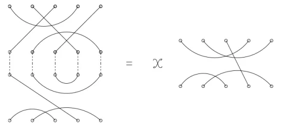
Figure 2.1: Example of a graph with Vf as set of vertices and f = 6.

2.2

B

(²n) - O(n) and Sp

duality

2.2.1 Brauer centralizer algebras

Let f ∈ N+ be fixed. Denote by Vf the datum of 2f spots in a plane, arranged

in two rows, one upon the other, each one of f aligned spots. Then consider the graphs with Vf as set of vertices and f edges, such that each vertex belongs to exactly one edge.

Figure 2.1 shows an example of such a graph for f = 6. Such graphs are named f -diagrams, denoting by ∆f the set of all of them. In general, we shall denote them by bold roman

letters. These set of the f -diagrams has the same cardinality of the set of the pairings of 2f elements, hence¯¯∆_f¯¯ = (2f − 1)!! = (2f − 1) · (2f − 3) · · · 5 · 3 · 1.

We shall label the vertices in Vf in two ways: either we label the spots in the upper

row with the numbers 1+_{, 2}+_{, . . . , f}+_{, in their natural order from left to right, and the}

spots in the lower row with the numbers 1−_{, 2}−_{, . . . , f}−_{, again from left to right, or we label}

them by setting i for i+ _{and f + j for j}− _{(for all i, j ∈ {1, 2, . . . , f }). Thus an f -diagram}

can also be described by specifying its set of edges: for instance, the 6-diagram in figure 2.1 is given by ©{1+_{, 4}+_{}, {3}−_{, 5}+_{}, {2}+_{, 4}−_{}, {5}−_{, 6}+_{}, {2}−_{, 6}−_{}, {3}+_{, 1}−_}ª_{. In general, given}

f -tuples i = (i1, i2, . . . , if) and j = (j1, j2, . . . , jf) such that {i1, . . . , if} ∪ {j1, . . . , jf} = Vf,

we call d_{i, j} the f -diagram obtained by joining i_k to j_k, for each k = 1, 2, . . . , f . So, the above diagram is di,j for i = {1+, 2+, 3+, 5+, 6+, 2−}, j = {4+, 4−, 1−, 3−, 5−, 6−}.

When looking at the edges of an f -diagram, we shall distinguish between those which link two vertices in the same row (upper or lower), which are named horizontal edges