Auger-PhotoElectron Coincidence Spectroscopy on magnetic thin films : a study of multiplet spin structure and electron correlation

(1)

Universit`

a degli Studi Roma Tre

Scuola Dottorale in Scienze Matematiche e Fisiche

Sezione di Fisica

XXVII Ciclo

Ph.D. Thesis

Auger-PhotoElectron Coincidence

Spectroscopy on magnetic thin films:

a study of multiplet spin structure

and electron correlation

Ph.D. Student: Marco Sbroscia

Supervisor: Prof. Giovanni Stefani

(2)

(3)

Per questo traguardo:

a pap`a Franco e a mamma Leonarda,

alla mia compagna Silvia, a me, il piccolo di casa.

Per la vita che ci attende: a nonno Franco e nonna Leonarda a nonno Mario e nonna Tiziana a zia Sara e zia Adele a zio Armando a mamma Silvia a pap`a Marco a Irene, la piccola di casa, la nostra nuova grande avventura.

(4)

(5)

`

E diﬃcile essere giusti perci`o cerco di essere onesto.

(6)

(7)

Introduction

Understanding and controlling electron correlation is one of the hardest task of modern physics. Electron-electron interaction is of particular interest because several highly intriguing phenomena like Ferro- and Antiferromag-netism (FM and AFM), Giant and Colossal Magnetoresistance or Super-conductivity are due to such a correlation. Since the advent of quantum mechanics, physicists have had to contend with diﬃculties of finding ana-lytical solutions to Schr¨odinger equation already for an atom as simple as Helium. In this simple case, for infinite nucleus mass approximation, the Hamiltonian of the system reads

H =−¯h 2 2m∇ 2 ⃗ r1 − Ze2 4πε0r1 − ¯ h2 2m∇ 2 ⃗ r2 − Ze2 4πε0r2 + e 2 4πε0r12

where the last term describes the interaction among the two electrons. Un-fortunately Coulomb interaction goes to zero as 1

r, where r represents the

distance between two charges and it does not allow to consider two electrons inside the same potential well completely independent. An example of phys-ical interest is the case of two electrons belonging to the same atomic site. Such an interaction term, and in the same manner every electron correlation term, produces an Hamiltonian not separable in single-particle contributions, making not possible to determine the exact eigenvalues as well as eigenstates of the system. In interpreting material properties local density approxima-tion (LDA) is a widely used frame for the independent quasi-particle picture. LDA is structured after a semiclassical mean-field theory approach and be-cause it is based on the use of a one-electron potential, it fails in describing strongly correlated systems. For example in a LDA picture a 3d-metal ox-ide Mott insulator is not properly described: FeO or CoO appears to have metallic behaviour instead of the insulator one pointed out experimentally. To include in the description the role played by interacting electrons, the so called density-functional theory (DFT) was developed. DFT is a theory de-voted to determine the electronic ground state structure for non-relativistic interacting electrons in an external potential v (⃗r). It is based on the

(12)

2

Introduction

Magnetic systems above transition temperature: is long- or short-range order lost? ple Hohengberg and Kohn lemma [1] which states that since the external potential influences the ground state energy of a many interacting electrons system and this potential is an unique functional of the one-particle elec-tronic charge density n (⃗r), the knowledge of such a physical quantity leads,

via a variational method, to the determination of the ground state itself [2]. Despite this step forward with respect to the original LDA approach, some aspects for interacting-electron systems are still missing: for NiO the pure DFT is not suitable to determine the right value of its band-gap [3, 4]. This is mainly because DFT neglects correlation among d-electrons, incorrectly accounting for occupancy of localized states. The main problem in applying DFT in the LDA to system with localised electrons resides in the depen-dence of the density functional from the exact potential. This latter seems to show discontinuities not reproduced in this method leading to the failure of the LDA in describing properties of strongly correlated materials, e.g. the band gap of Mott insulators [5, and ref. therein] as mentioned before. Thus, what was said just above makes clear the necessity to go beyond any single-particle approach to properly describe such systems, overcoming methods in which the interaction among electrons is approximated via a mean field or introduced in a pure perturbative manner.

These few examples have been proposed just to underline the importance of taking into account the electron correlation. This is more relevant in the case of magnetic systems where the electron-electron interaction is the ori-gin of such properties. In this thesis a correlation-sensitive spectroscopic technique like Auger PhotoElectron Coincidence Spectroscopy is applied to magnetic thin films with the aim to validate theoretical models which de-scribes the electron spin coupling contributing to the Auger transition and to access an unambiguous assignment of the several final state spin terms allowing for a deeper understanding of the electron correlation and magnetic properties at atomic scale.

Magnetic systems above transition

tempera-ture: is long- or short-range order lost?

Highly correlated systems are occupying a relevant place in modern physics not only because a proper and complete description of their properties has not been reached yet, but also for their possible use in new devices. In this latter field a central role is played by magnetic thin films and heterostructures for their application in spintronics, hence monitoring the magnetic phase tran-sition becomes a fundamental aspect. A highly debated issue is the origin

(13)

Introduction

Magnetic systems above transition temperature: is long- or short-range

order lost? 3

of magnetic properties of solids at the atomic level or, in other words, what happens to magnetic and electronic structures, from a microscopic viewpoint, when a sample exceeds its own magnetic transition temperature (Curie tem-perature (TC) for FM, N´eel temperature (TN) for AFM). It is well known

that when a FM or an AFM material is well below this critical tempera-ture it shows a long range magnetic order throughout the solid. When the solid overcomes the transition temperature the long-range order is lost, but what happens at atomic scale is still far from the comprehension and, at the state of the art, conflicting experimental evidences are present. Mook et al. [6] performing neutron scattering on a FM Ni specimen showed that spin-wave excitations could be observed at temperature higher than Curie point relating this to the persistence of spin correlation well above the transition temperature. Of the same tendency are the photoemission results from bulk [7, 8] as well as surface [9] states of Ni. In these cases photoemission spec-tra show the presence of two distinct peaks associated to the spin-up and spin-down splitted bands. Increasing the temperature, exceeding the Curie point, the non-collapse of these two structures characterising the spectra re-veals the persistence of exchange splitting and consequently the existence of a short-range magnetic order above TC. Hopster et al. [10] found an

ex-perimental temperature-dependence of exchange splitting (decreasing of the exchange splitting upon increasing the temperature) in Ni that cannot be concordant with the temperature-independent theoretical models supported by the aforementioned results. So the situation is far from being clear be-cause the exchange-splitting temperature-dependence is strongly dependent from the theoretical approach used in interpreting photoemission spectra [9]. Contradictions are not finished yet. In a magnetic material, below the phase transition temperature, exchange interaction splits the valence band in two pure spin bands. Spin band splitting derives from the proper balance of exchange-energy gain (the interaction among electron’s spins) and the ki-netic energy variation due to Pauli exclusion principle (electrons with the same spin have to be in diﬀerent(⃗k, E(⃗k))band points). In such a scenario the characteristic FM or AFM behaviour is described, in an Heisenberg model approach, through an Hamiltonian term like

Eex=−

∑

i̸=j

J_exij S⃗i· ⃗Sj

where the sum runs over all the atomic sites, ⃗Si and ⃗Sj are spins of two

diﬀerent interacting electrons, while J_exij is the exchange integral and the external field contribution is neglected. The exchange integral takes into account the FM or AFM nature of the system. The minimisation of the exchange energy implies that if Jex > 0 the spins of interacting electrons are

(14)

4

Introduction

Magnetic systems above transition temperature: is long- or short-range order lost?

coupled in a parallel alignment favouring a FM order, while if Jex < 0 an

antiparallel coupling is favoured leading to an AFM order. Such a model derives from a local description of the (anti-) ferromagnetism and puts in ev-idence the role of the electron correlation in such phenomena. Anyway this model can be integrated by a band theory approach in which the magnetic properties of a system are derived from their band structure, the so called Stoner model. For a spin polarised sample the density of states (DOS) shows two different subbands accounting for spin-up and spin-down populations. These two bands are energy shifted because of the exchange interaction and this splitting is reduced upon increasing the temperature. Once the sam-ple’s temperature exceeds the transition point these two bands coalesce, as predict by long-range-order models. Magnetic excitations, like single-particle spin flip (Stoner excitation) or collective excitations (spin-waves or magnons) [11], are expected to be sensitive to such changes. It is expected that differ-ences in the spin bands splitting leads to a temperature dependence in the energy-vs-momentum plot of these quasi-particles, but on the contrary such a dependence has not been observed in neutron scattering experiments by Mook et al. [6]. Of the same advice is the work by Kirschner and Langen-bach [12] in which exchange splitting in Ni has been shown to be temper-ature independent using high-resolution spin-polarised electron-energy-loss spectroscopy. Spin-resolved photoemission and inverse-photoemission exper-iments performed on Fe [13, 14] pointed out a complex scenario: the collapse of magnetic order depends upon the sampled point in k-space, for example studying the exchange splitting of empty bands it has been shown that for an high symmetry phase-space point, namely the H point, of a bcc Fe sample majority and minority bands merge together upon approaching the Curie point from below, while for the same crystal, sampling two other different phase-space points, a non-collapsing behaviour is found. These complications make difficult to understand the itinerant-electron ferromagnetism1. During the ’90s other experiments were performed in order to clarify the situation which, however, remained the same: temperature and wave-vector depen-dence of exchange splitting [15, 16] and collapse of band-splitting approaching the Curie temperature observed in inverse photoemission [17] are in contrast with the presence of local moments of 3d-character and spin polarisation above TC [18] still making not possible to properly interpret magnetism.

Re-cently the temperature evolution of itinerant ferromagnetism [19, 20] seemed to be in agreement with the persistence of local magnetic moment well above the Curie point, but, again, the issue about whether FM originates from local

1_{An itinerant ferromagnet is a system whose magnetic properties are characterised by}

(15)

Introduction

Probing electron correlation: the advent of electron-pair detection

experiments 5

moment or itinerant electrons is of pivotal importance. In the last years ef-forts have been made in trying to answer it unequivocally, but unfortunately a complete description of magnetism remains controversial.

Probing electron correlation:

the advent of

electron-pair detection experiments

As discussed in the previous sections, a complete understanding of mag-netism around the transition temperature has not been reached yet. As a consequence theoretical models are able to predict only a few aspects at a time of the physical phenomena observed experimentally. The Stoner-Wohlfarth approach [21, and ref. therein], based on the assumption that the exchange energy is proportional to the square of the magnetisation, takes into account a reduction of the exchange interaction upon increasing the temper-ature reaching a paramagnetic state at the Curie point. On the contrary, in local fluctuating band theories, the magnetic phase transition is driven by the transverse fluctuations like the spin-waves. In this case, for an itin-erant ferromagnet, because of the delocalised nature of the electronic wave functions, the Si2, where Si represents the total spin density operator for

the i-th lattice site, does not correspond to a sharp quantum number. This means that fluctuations among diﬀerent atomic sites are able to destroy the long-range magnetic order, preserving local magnetic moments above TC.

In order to overcome this controversial picture, in the last decades ef-forts have been dedicated to the description of strongly correlated mate-rial properties. As mentioned before the LDA scheme, even considering the DFT approach, is not completely satisfactory because it fails in describing correlation among the d- and f -electrons while they play a critical role in magnetism. In this direction the first refinement has been the introduction of the Hubbard parameter U , which describes Coulomb energy interaction among two electrons at the same lattice site [22], in the so called LDA+U scheme [23, 5, 24] as well as the introduction of the dynamical mean field theory (DMFT) approach [25, 26], but for the comprehension of magnetism in solids, the capability to completely describe the itinerant electrons be-haviour plays a crucial role. The nature of these electrons can be classified comparing the same U parameter coming from the Hubbard Hamiltonian [22] with respect to the band width W to which they belong. In systems like magnetic thin films of 3d metal and their oxides, where U , W and the exchange interaction ∆, responsible for majority and minority spin bands splitting, are of the same magnitude, it is not possible to neglect the mutual

(16)

6

Introduction

Probing electron correlation: the advent of electron-pair detection experiments

electron repulsion.

The difficulties in understanding magnetism and, more in general, Coulomb interaction in many-body effects, originates not only from the theoretical side, indeed the most common and used spectroscopic techniques are based on single-particle interpretation. For example photoemission spectroscopy involve a single-particle dipole matrix element. Despite very appealing, be-cause the quasi-particle band structure can be probed, these single electron spectroscopies give us information about correlation only indirectly, e.g. via the satellite peaks in photoemission spectra, but this seems not to be enough to fully understand electron correlation and related phenomena. In the last forty years efforts have been made in developing new experimental techniques able to directly probe electron correlation. In this scenario the electron-pair emission based experiments like direct and core-resonant Double Photoemis-sion seem to be successful. In this kind of experiments two or more electrons coming from the same interaction process between the sample and the probe (electrons or photons) are collected. This means that after excitation the target falls in a final state characterised by two or more interacting holes in the valence band, giving access to correlation effects. These techniques are suitable for probing matter in its various states of aggregation: in atomic, molecular or solid form.

In a direct double photoemission process the photon absorption leads to the emission of two electrons according to

¯

hω + A → A++(v−1v−1)+ e−+ e−

where an impinging photon represented by its energy ¯hω and a neutral

charged atom target in its ground state, A, form the initial state. In the final state are present a doubly ionised atom A++(v−1v−1) with two holes in valence levels and two electrons emitted in the continuum. These two electrons can share the excess energy available in the final state.

It is possible to get the same final state via the decay of a core-hole, that leads to the emission of an Auger electron coupled to the photoemitted one. In this case the double photoionisation process is termed as core-resonant and the reaction reads

¯

hω + A → A+(c−1)+ e−→ A++(v−1v−1)+ e−+ e−

where A+_(c−1_{) + e}− _{represent the intermediate state where a core-hole is}

produced in the target and an electron is in the continuum. For this core-ionised state the decay, for our purpose, is driven by an Auger emission. This is the case in the Auger PhotoElectron Coincidence Spectroscopy (APECS) [27].

(17)

Introduction

How APECS can access magnetic properties from a local viewpoint 7

Written in this form, the reaction can be interpreted in a two-step model where the Auger emission takes place from a stationary state and can be treated separately with respect to the preceeding photoionisation process, hence this is possible only if the core-hole lifetime is long enough to allow the relaxation of the other excitations, otherwise a one-step process, with the emission of two electrons sharing the excess energy, follows the photon absorption [28, 29, 30].

In an APECS experiment two electrons out-coming from the sample and generated in a unique radiation-matter interaction event are collected in a time-correlated and energy-resolved fashion. After the photon absorption a photoelectron is emitted in the continuum and the sample goes in a core-ionised state. In the target, via an autoionisation process driven by Coulomb interaction, the core-hole decays leading to the emission of a second, Auger, electron coupled to the first one. The photoemission process, when the photo-electron is discriminated in angle with respect to linear polarisation, prepares a proper subset of core-ionised states in the target. The collection of Auger electrons in time coincidence with photoelectrons of a specific energy allows to measure the partial Auger yield associated to the decay channel of only that particular subset of ionised states.

It is clear that such an experimental approach highlights 2-electrons and 2-holes material properties, in other words properties of both the electron-pair in the continuum and the interacting final state holes in valence band (or levels) must be described via a 2-quasi-particle wavefunction. For this reason the interpretation of correlation spectroscopies results are related to a 2-particle density of states (2-DOS). Theoretical works devoted to the de-termination of 2-DOS have made their appearance since late ’70s with the pioneering works of Cini and Sawatzky [31, 32] undergoing later developments to be suitable not only for closed shells [33].

How APECS can access magnetic properties

from a local viewpoint

As mentioned before, d-electrons and d-holes dictate the magnetic properties for transition metals and their oxides. For this reason it is fundamental to probe the behaviour of their valence electrons. Magnetic quantum numbers of the two, or more, final state holes are related to those of the ejected electrons, which are responsible, through their spin coupling, for the magnetic properties of the system. Hence, probing the d-holes spin coupling, magnetic information can be unravelled.

(18)

8

Introduction

How APECS can access magnetic properties from a local viewpoint

The angular electron emission is such that electrons characterised by par-tial waves with different projections m of the angular momentum, i.e. elec-trons belonging to different magnetic sublevels, are mainly emitted at differ-ent angles with respect to the electric vector of linearly polarised light, which acts as quantisation axis [29, figure 4]. Both the selection rules for the pho-toemission process2 _{and for the Auger [34] put in correlation the magnetic}

quantum numbers of the partial waves of the emitted electrons with those of the valence holes in the final state [29]. In this way, combining the angular emission pattern with the selection rules, it is straightforward to differently weighting individual total spin contributions to the final state without any spin detection, but just collecting electrons under different kinematic condi-tions. Hence performing APECS experiments in an Angle-Resolved fashion (AR-APECS), that means upon changing the experimental geometry, leads to collect electron-pairs arising from different multiplet spin terms3.

It has been shown recently by Stefani and co-workers [35] how the appli-cation of this coincidence spectroscopy to magnetic systems makes possible to get information about their magnetic state. The spectral difference in AR-APECS spectra collected in different kinematics gives a Dichroic Effect called DEAR-APECS, by means of which it is possible to access the final state holes spin configuration [36] unravelling individual multiplet contribu-tions to the Auger spectrum. It has been shown that the DEAR-APECS effect is sensitive to the magnetic order of the systems under investigation, i.e. while it is present when a magnetic sample is below its phase transition temperature, it disappears exceeding such a value [37].

APECS is a core-excitation based technique and, in the same manner of other core-emission based spectroscopies, has a correlation length dictated by the spatial extension of the core-hole wavefunction. This means that APECS brings informations on the systems at atomic scale. This makes APECS a powerful tool to probe and monitor the magnetic phase transition from a local viewpoint overcoming limitations induced by the necessity of long-range order required by most electron spectroscopies and without having to rely on crystal periodicity or thermodynamical issues.

This work is devoted to the study of electron correlation in strongly

cor-2_{Optical dipole selection rules: ∆l =}_{±1 with l angular momentum and ∆m = 0 in the}

case of linearly polarised light.

3_{When two or more spins of interacting quasi-particles are coupled the angular momenta}

combination rules give back more than one total-spin state. For example combining two

|1

2⟩ spins the total spins accessible are |0⟩ and |1⟩ the well known Singlet and Triplet

states. In the same way combining for example four |1₂⟩ spins besides the Singlet and Triplet contributions rises the Quintet one. When considered in their totality these spin states are known as spins’ multiplets.

(19)

Introduction

How APECS can access magnetic properties from a local viewpoint 9

related systems like magnetic thin films in the few monolayers regime. We performed AR-APECS experiments on both FM and AFM systems in order to unravel spin multiplets and the eﬀects of electron correlation on the final state spin contributions. Exploiting both the local sensitivity and the spin selectivity of the AR-APECS will be possible to contribute to the issue about the loss of short-range magnetic order exceeding the transition temperature for both FM and AFM systems.

(20)

10

Introduction

(21)

Chapter 1

Magnetic properties of solids

Man’s encounter with magnetism is rooted in ancient time. A first hint of such a still vivid relation is given in the “Thales of Miletus” (about 634-546 BC) in which the fascinating property of the “lodestone”, today commonly called magnetite, Fe3O4, of attracting iron was first described. History of

magnetism found location also in China where the first instrument known to be a compass found its birth: it has been realised modeling a piece of lodestone into a spoon shape and placing it onto a bronze plate, as reported in figure 1.1. The handle of this spoon pointed, misteriously, to the South. Pliny the Elder (23-79 AD) in his Historia Naturalis traces the term magnet to a shepherd called Magnes, who discovered the “attractive” power of some stones putting his iron-nailed cane on the ground. Maybe the most important medieval study on magnetism still remain the epistle “De Magnete” by Peter Peregrinus (title page in figure 1.2a) which introduces the concept of magnetic poles, but starting from 1600 AD the reference text was the “De Magnete” by William Gilbert (title page in figure 1.2b). Nowadays magnetism is one of the most important field of research because it aﬀects our everyday-life. This fact gives to magnetism a special place and a new vitality, also due to the fact that is a field that is still undergoing developments.

1.1 Magnetism in three-dimensional systems

Magnetic material are with no doubts among the most important and intrigu-ing materials in nature and a microscopic investigation of such phenomenon is of pivotal interest. A magnetic medium can be described exploiting the so called constitutive equations, particularly by means of the magnetic perme-ability µ and the susceptibility χ. Such quantities are related to the magnetic field H, the magnetic induction B and the magnetisation M according to the

(22)

12

Magnetic properties of solids

Magnetism in three-dimensional systems

Figure 1.1: Working model of the first instrument known as a compass composed by a magnetic lodestone spoon and a bronze plate. Image from the web.

(a) Title page of the epistle De

Mag-nete by Peter Peregrinus in 1296 in

the reprint of 1558, Gasser ed. Ger-many. Figure from the web.

(b) Title page of the “De Magnete” by William Gilbert in 1600. Figure from the web.

(23)

Magnetism in three-dimensional systems 13

following equations [38, p. 15]: ⃗ B = µ ⃗H ⃗ M = χ ⃗H ⃗ B = H + 4π ⃗⃗ M = (1 + 4πχ) ⃗H.

From a macroscopic viewpoint the magnetisation M represents the linear response to the application of an external field and it finds its origin in the magnetisation current induced by the action of the Lorentz’s force upon the charges constituting the system. From this viewpoint a preliminary, but not satisfactory, connection with the microscopic nature of magnetism can be seen. For this reason the susceptibility represents a quantity able to discriminate upon diﬀerent magnetic behaviors, allowing to classification of diﬀerent magnetic materials.

χ < 0 Diamagnetic i.e. He, Ne, NaCl, Cu

0 < χ << 1 Paramagnetic (PM) i.e. Na, Al Antiferromagnetic (AFM) i.e. NiO, FeO

χ >> 1 Ferromagnetic (FM) i.e. Fe, Co, Ni

Ferrimagnetic (Fim) i.e. Fe3O4

A diamagnetic substance, once immersed in an external magnetic field, reacts producing a magnetic moment opposite to the field, thus showing a negative susceptibility. The classical theory was formalised by Langevin in 1905 [39] on the base of the work of Amp´ere and Weber. In the same paper Langevin put down the theory for paramagnetic systems. In this case he assumed the same net magnetic moment µ for each atom of the specimen. These magnetic moments result randomised in the absence of an applied field, so the net magnetization of the sample is zero. If an external field is applied, these atomic moments tend to align to the field direction, but thermal ag-itation of the atoms opposes this tendency and randomises the moments. The result is only propensity to the alignment in the field direction, and therefore only a small positive susceptibility is obtained. Upon increasing the temperature this randomising eﬀect is increased. Ferromagnetic and an-tiferromagnetic are indeed substances which in the high-temperature regime

(24)

14

show a paramagnetic behavior, but at low temperature (lower than a crit-ical value characteristic for each system) they show a magnetic order even in absence of an external applied field. In the case of a ferromagnetic mate-rial this order is accompanied by a large net spontaneous magnetisation, on the contrary for an antiferromagnetic system the net magnetisation is null at any temperature, so it is possible to distinguish it from a paramagnetic specimen only with a very close investigation in a wide temperature range. Ferrimagnetism is the case of double oxide of iron and other metals. Like ferromagnetic materials they show a net spontaneous magnetisation which rises from a particular spin alignment: spins are coupled antiferromagneti-cally but the two FM sublattices show diﬀerent magnitude. Because of these reasons they are a class apart.

In the following we will examine the intensive properties such as suscepti-bility and saturation magnetisation of Ferromagnetic and Antiferromagnetic substances, which are relevant for technological applications and are the kind of magnetic substances investigated in this thesis. These properties are not dependent on details of structural elements like lattice imperfections, grain size, crystal orientation or presence of impurities. Following the temperature dependence of such quantities a great clue on the magnetic nature of these systems can be achieved.

1.1.1 Ferromagnetism

Some substances, very common indeed like Iron or Cobalt, have shown a par-ticular behavior with respect to others magnetic systems. A typical paramag-net is characterised by a paramag-net magparamag-netisation if dived into an external magparamag-netic field, but it shows no magnetism once removed from the field, while for a fer-romagnet a magnetic ordering is preserved even if no external magnetic field is applied. Such substances are termed as Ferromagnet or Antiferromagnet. For these systems the existence of a spontaneous magnetic order suggests that their ground state must be characterised by a well defined orientation of the magnetic dipoles. Such dipoles can be very large and they are responsible for the macroscopic permanent net magnetisation. This magnetic order can be removed only heating the sample exceeding a certain temperature, typical for each system, termed as critical temperature, Tc. This temperature acts

as watershed between the (Anti-) Ferromagnetic state and the paramagnetic one. In order to get more details on the nature of the interaction respon-sible for this behavior, let us refer to table 1.1 in which the magnetisation at T = 0 K, the magnetic moment and the critical temperature are given. In a magnetic system the dipole-dipole interaction has the tendency to line up the dipoles: a dipole influenced by the dipolar field of another magnetic

(25)

M @ T = 0 K (gauss) _µµ B Tc (K) Fe 1752 2.219 1043 Co 1446 1.715 1394 Ni 510 0.604 630 Gd 1980 7.12 293

Table 1.1: Magnetisation, magnetic moment and Curie temperature for the most common ferromagnets. Values from [40, chapter XVII].

dipole is aﬀected by a torque which tends to align this two dipoles. Such an interaction is of the form ∼ µ1µ2

r3 and it is possible to estimate typical

energy contribution of this classical interaction of the order of ∼ 0.1 meV. The critical temperature (or Curie temperature for a ferromagnet) reported in table 1.1 are of the order of∼ 100 meV, hence they cannot be interpreted in terms of the dipole-dipole interaction. No real progress in understanding magnetism was made until P. Weiss proposed the idea of an internal field usually called molecular field [41] responsible for the dipole alignment. In such a mean field theory the magnetisation is not only due to the external field, but a molecular field play a role:

H_eﬀ = H + λM

where the last terms takes into account for this field generated by the aligned dipoles. Under this assumption the magnetisation can be expressed as [40, chapter XVII] M = N V µ0tgh [ µ0(H + λM ) KBT ] (1.1)

where M is the magnetisation, µ0 = gµBJ is the magnetic moment given as

the product of the gyromagnetic factor g, the Bohr magneton and the total angular momentum of the ion, N_V the number density of ions in the system and KBT the thermal energy. It has been considered the interesting case1

for J = 1₂ and g = 2 instead of using the complete Brillouin function for the sake of simplicity. This equation allows to determine the magnetisation of a ferromagnet in absence of the external field, H = 0. Under this restriction equation (1.1) is reduced to:

M = N V µ0tgh ( µ0λM KBT ) . (1.2) 1_{See figure 1.5}

(26)

16

Figure 1.3: The solution of equation (1.3) is given in figure in terms of rela-tive magnetisation as a function of the dimensionless α parameter. Curve 1 is the Langevin function. Solutions for three temperature values are given. Image redrawn from [38].

Such an equation has a standard way to be solved: defining α = µ0λM

KBT and

Tc=

µ2₀λN

V KB equation (1.2) can be rewritten as

tgh(α) = αT

Tc

(1.3)

which can be graphically solved as given in figure 1.3: the Langevin curve labeled as 1, that represents the relative magnetisation (here M0 is the

sat-uration magnetisation), is reported with a plot of equation (1.3) for three diﬀerent temperatures T2, T3 and T4 in the T2 < T3 < T4 relation. In the

case T = T3 = Tc the straight line is tangent to the Langevin function in α = 0 so the slope of line 3 determines the Curie temperature of the system.

Increasing the temperature, as in the case of line 4, the only intersection point between this two curves is in the origin, i.e. the case M = 0 that is not of interest. The most intriguing case is given by line 2 for which a non trivial solution for equation (1.3) is present. The point P represents the spontaneous magnetisation, expressed as a fraction of the saturation value, achieved at that temperature.

Let us now focus only on the solution at T = T2. The trivial solution

M = 0 represents an unstable state because the slightest applied field, e.g.

the Earth’s field, will magnetize the system to a certain point, A in figure 1.4. At this point a magnetsation M = A must be due to a molecular field

(27)

Figure 1.4: Schematic representation of the spontaneous magnetisation process due to the molecular field. Image from [38].

Hm = λM = B in reference to figure 1.4. Anyway such a field must produce a magnetsation M = C and so on up to the point P that represent a stable point at which the sample results spontaneously magnetised. The magneti-sation of these ferromagnetic systems as a function of the temperature shows a trend similar to those reported in figure 1.5. In such a figure σs

σ0 expresses

the magnetisation in terms of the specific magnetisation according to the relations [38] σs σ0 = Msρ0 M0ρs σ σ0 = (_{J + 1} 3J ) (_T Tc ) α′ α′ = µHH KBT

where ρs(0) is the density of the system at temperature T (T = 0 K), J is the

total angular momentum of the ion and µH the projection along the field of

the magnetic moment. Figure 1.5 clarify the role of the critical temperature

Tc, while the system taken below such a value shows a spontaneous

magneti-sation, on the contrary it shows no magnetic order exceeding that critical point. Of course this two diﬀerent magnetic states follow two diﬀerent laws: approaching the Curie temperature from below the magnetisation scales with a power law temperature dependence, while approaching it from above the typical Curie-Weiss law describes the paramagnetic behavior shown by the

(28)

18

Figure 1.5: Relative saturation magnetisation as a function of the temperature for Iron, Nickel and Cobalt. The solid lines are calculations for diﬀerent values of the total angular momentum J . Image from [38].

system [40, chapter XVII]

     M = N_V µ0_TT_c √ 3(1− _TT c ) if T → T_c− M = N_V µ20H KB(T−Tc) if T → T + c .

Figure 1.5 gives also information about the angular momentum, J , depen-dence of the magnetisation: the best agreement between the experimental values an the theoretical calculations is obtained for the total angular mo-mentum J = 1₂ that means the magnetic moment is entirely due to the spins, with no orbital contribution. Hence it is possible to state that ferromag-netism in transition metals is due essentially to electron spin [38].

The Weiss theory of the molecular field gives no explanation about the origin of this field, simply it relates via a proportionality law this field and the existing magnetisation, underlining the cooperative nature of the phe-nomenon, as shown also in figure 1.5 in which the spontaneous magnetisa-tion decreases upon the increasing of the temperature. Only in 1928 this origin started to be understood, with the brilliant hypothesis by Heisenberg, who proposed that the spin alignment throughout the solid was due to the exchange interaction, so a purely quantum eﬀect with macroscopic mani-festation. Exchange forces depend on the relative spin orientation of two

(29)

interacting electrons. It is a consequence of the Pauli exclusion principle2 applied to these two interacting electrons as a whole system. According to this principle these two electrons cannot occupy the same energy level unless they are provided of two opposite spins. This interaction arises from the Coulomb force, so it has basically an electrostatic origin.

Let us suppose two diﬀerent atomic sites labeled as A and B. The total Hamiltonian can be expressed as

HA+ HB+ H1,2

considering HA (B) the single-particle Hamiltonian for an electron in the

atomic site A (B) and where

H1,2 =− e2 |⃗r1− ⃗rB| − e2 |⃗r2− ⃗rA| + e 2 |⃗r1− ⃗r2| .

The two-electrons Hamiltonian allows two diﬀerent total spin states, the Singlet with S = 0 and the Triplet with S = 1, energy shifted by twice the exchange integral [40, chapter XVII]

E(S = 0)− E(S = 1) = 2Jex.

Heisenberg intuition was to attribute ferromagnetism to the direct spin-spin interaction that can be described with an Hamiltonian term like

H =− ∑

m̸=n

J_mnexS⃗m· ⃗Sn.

Exchange interaction drops rapidly to zero upon increasing the separation between the two interacting electrons, thus it is possible to simplify this term reducing the sum over all the possible atomic site to the nearest-neighbor. In the simplest case let us consider only the z-component (along the quantisation axis) of the spin. Assuming also that the exchange integral is the same for all these neighbours, that means assuming an isotropic substance, the Heisenberg model is reduced to the Ising one:

H_I =−Jex∑

m,i

S_mzS_m+iz (1.4)

where the index m runs over all the atomic sites and i over the nearest-neighbours. It is clear that a positive exchange integral, which is a rare

2_{The name exchange comes from the fact that two electrons are completely}

indistin-guishable so the energy contribution in which they exchange their role must be accounted for.

(30)

20

condition, is necessary for a ferromagnetic alignment of the spins, because if

Jex > 0 a parallel alignment of the spins leads to a minimum in the exchange

energy, on the contrary in the case of Jex < 0 an antiparallel,

antiferromag-netic, alignment is favored. Of course the exchange integral, if positive, is proportional to the Curie temperature. This is very simple to understand because it requires a large thermal energy to destroy the spin alignment held by a strong exchange interaction. Anyway it is possible to put this statement on a more quantitative ground [38]:

Jex = 3KBTc

2zS(S + 1)

where z is the coordination number, i.e. the nearest-neighbor, and S the spin. Exchange forces depend mainly on interatomic distances and not on any geometrical arrangement of the atomic sites, thus crystallinity is not a required condition for forromagnetism. The first discovery of ferromagnetism in an amorphous sample goes back to 1965 [42].

In discussing about the spin alignment in a ferromagnet a marginal role has been given to the dipole-dipole interaction. Such a classical interaction term contribute with an energy given by [38, p. 365]:

∆E = µ⃗1µ⃗2

r3 −

3

r3( ⃗µ1· ˆr)( ⃗µ2· ˆr)

where ⃗r is the distance between the two dipoles ⃗µ1 and ⃗µ2. This dipolar

interaction drops to zero as _r13 slower with respect to the exchange integral

and at a macroscopic level it is responsible for the formation of the so called “Weiss domains”. A Weiss domain is a portion of the sample in which a certain number of spins are aligned to each other, but two adjacent domains can have two different orientation of the net magnetic moment. This is due to the fact that the exchange interaction forces the spins to lie parallel to each other, but a configuration with all the spins aligned is not favored by the dipole-dipole term. Thus a proper balance of this two contribution leads to the formation of different domains in order to gain energy from the dipole-dipole interaction among different domains and the gain from the spin coupling inside a single domain. The only expenses are in the formation of the separation surfaces between domains, the so called “domain walls”.

This domain structure is able to account for the absence of spontaneous magnetisation in a ferromagnet above the Curie temperature: starting with a system showing a net magnetisation, i.e. there is a propensity in the domain alignment, upon increasing the temperature the orientation of the diﬀerent domains starts to randomise, reaching a condition of a null average net magnetisation once approached the Curie point.

(31)

The Stoner model: a brief description

In the previous paragraph a brief description of the local Weiss theory for ferromagnetism has been given. Such a theory for the 3d-transition metal is adequately integrated by a so called band theory. The simplest band-model is often referred as Stoner-Wohlfarth-Slater-model (SWS-model) which is based on the one-electron density of state considering separately for the two possible spin orientation (up (↑) or down (↓)). Due to the exchange interaction which prevents that an electron can be approached from another with the same spin, the eﬀective charge density of electrons with the same spin orientation in the neighborhood is reduced. In the Stoner model this is taken into account introducing an energy renormalisation as follow [43, chapter 9 section 4]:

E_↑(⃗k) = E(⃗k)−In↑

N E_↓(⃗k) = E(⃗k)−In↓

N

where E(⃗k) are the normal one-electron energy-bands, n_{↑ (↓)} the number of electrons with the corresponding spin and N the total number of atoms. The exchange correlation eﬀect is taken into account with the Stoner parameter

I. A k-independent subband splitting results from this model as depicted

in figure 1.6. In the presence of a molecular field the centers of the two subbands with opposite spins are separated by the exchange splitting ∆. At T = 0 K all the electron states are filled up to the Fermi level, so it results convenient to refers to electrons as majority or minority, according to the excess of one kind of spins with respect to the other. The microscopic ferromagnetic moment originates from the excess of majority spin over the number of minority spins:

|⃗m| = µB(n_maj− n_min).

The occurrence of spontaneous magnetism below Tc can be explained as

follow [43, pp. 477-478]: local fluctuations in the spin orientation below the Curie point lead to a momentary polarisation responsible for the spin alignment into a magnetic order, which in turn is responsible, because of energetics, of the majority and minority band splitting.

1.1.2 Antiferromagnetism

Besides the ferromagnetism there is another intriguing type of magnetic or-der termed as antiferromagnetism. An antiferromagnet (AFM) is a substance

(32)

22

Figure 1.6: The Stoner model for the 3d-metal is reported. Occupied electron states below the Fermi energy EF are shown shaded. The spin band with the

largest number of electrons is termed as majority spin band, the other as minority. The centers of the two subbands are separated by the exchange splitting ∆. The labels “spin-up” and “spin-down” only have a meaning in conjunction with a quan-tization direction, which is taken to be the direction of the external field. Minority spins always point in the direction of the magnetisation M. The magnetic moment

|⃗m| is determined by the diﬀerence in the number of majority and minority spins.

(33)

Figure 1.7: Temperature dependence of susceptibility and its inverse for an AFM system: schematic representation. AF and P refer to antiferromagnetic and para-magnetic respectively. θ is the temperature value, proportional to the molecular field, at which the susceptibility diverges in the Curie-Weiss law. The N´eel tem-perature TN is also reported. Image from [38, chapter 5].

characterised by a susceptibility3_{which varies in a peculiar way with the}

tem-perature, appearing, at first glance, like an anomalous paramagnet. In figure 1.7 the susceptibility χ as a function of the temperature in an AFM is re-ported. Starting from the high-temperature limit, the susceptibility increases as the temperature decreases, reaching a maximum at a critical temperature called N´eel temperature, TN. Going further in decreasing the temperature

under TN the susceptibility starts to decrease. Closer studies have put in

evidence that such systems requires a proper classification. Such substances show themselves as a paramagnet above TN and as an AFM below it.

Tran-sition metal oxides are one of such a kind of systems and some values for their TN are given in table 1.2.

The theory about antiferromagnetism found its origin in 1932 with the work of L. N´eel [45]. In his work he applied the Weiss molecular field theory, discussed above, to the problem of antiferromagnetism. In figure 1.7 the straight dashed line extrapolates to a negative temperature at _χ1 = 0

χ = C

T + θ =

C

T − (−θ)

in other words obeying the Curie-Weiss law but with a negative temperature.

3_{In general, upon application of an external magnetic field H, a specimen acquires a}

(34)

24

Metal ion arrangement TN (K) −θ (K)

FeO fcc 198 570

CoO fcc 293 280

NiO fcc 523 3000

MnO fcc 122 610

Table 1.2: Crystal symmetry, N´eel temperature and −θ temperature ex-trapolation for the most common transition metal oxides antiferromagnets. Values from [38, chapter 5].

θ = ρCγ hence is proportional to the molecular field coeﬃcient (see ref. [38,

p. 97, eqn (3.22)]) and this means that in the paramagnetic region the molecular field is opposite to the applied field H; whereas H tends to align the ionic moments the molecular field acts to disalign them. At atomic scale any tendency of ionic moment to point in one direction is immediately counteracted by the tendency of the adjacent moment to point in the opposite direction [38, chapter 5]. According to equation (1.4) such systems have a negative exchange integral. Below the critical temperature this tendency to align in antiparallel fashion the magnetic moments throughout the solid is strong enough to survive the thermal energy even with no applied field. Such a strength increases upon decreasing the temperature below TN down

to T = 0 K where the antiparallel alignment results perfect. It is now clear that an AFM system has no spontaneous net magnetisation and can acquire a moment only under the eﬀect of a high external magnetic field. It is also clear that the N´eel temperature TN play a role equivalent to the Curie temperature

for a ferromagnet dividing the magnetic ordered phase and the paramagnetic one.

Almost all AFM systems are electrically insulators or semiconductors. This means that they contain no free charges, hence their magnetism is dic-tated by localised electrons belonging particular ions. Therefore the molecu-lar field theory, that is a localised-moment theory, is expected to better fit the case of antiferromagnetism with respect to the ferromagnetism [38, p. 154]. Let us divide the entire AFM lattice in two identical sublattices, namely A and B, such that all nearest-neignbours of sublattice A are B sites and vice versa. In doing so only the magnetic ions arrangement is taken into account. In both of these sublattices a ferromagnetic arrangement is present. In the case of a simple cubic whole lattice two interpenetrating fcc (face-centered cubic) sublattices in the well-known NaCl structure are obtained for A and B, while in the case of a compete bcc (body-centered cubic) lattice the

(35)

re-Magnetic properties of solids

sulting sublattices A and B show a simple cubic structure. In the case of the entire AFM lattice is fcc there is no simple partition for the two sublattices A and B in order to get all nearest-neighbors of an A site belonging to B and vice versa [40, p. 635]. The Weiss theory can be applied to each sublattice assuming that the eﬀective field acting on a site A contains a cooperative con-tribution proportional and opposite to the magnetisation on the B sublattice and vice versa. Let us also assume that the nearest-neighbor interaction is of the type AB (BA) and the second-nearest-neighbor, AA (BB), is again antiferromagnetic. In this case we have two molecular fields to deal with [38, chapter 5]:

H_mA= λM_B

H_mB = λM_A.

So the eﬀective field on the two sublattices are [40, chapter XVII]:

⃗

H_A(eﬀ) = ⃗H− λ1M⃗B− λ2M⃗A

⃗

H_B(eﬀ) = ⃗H− λ1M⃗A− λ2M⃗B (1.5)

where H is the external field, M_A(B) the magnetisation of sublattice A (B) and λ1, λ2 two positive phenomenological constants (λ2 can be also null or

negative, but |λ2| < λ1) which account for the first- and

second-nearest-neighbor interaction respectively.

It must be taken into account that once applied a field above TN each

sublattice becomes magnetised in the same direction of the applied field, but the molecular fields act in the opposite direction of the applied field reducing the two sublattice, i.e. the net, magnetisation with respect to the case of an ideal paramagnet. In this condition the susceptibility of the systems follows the Curie-Weiss law but results reduced with respect to the non-interacting case (λ1 = λ2 = 0 = θ) as expressed in the following equation [40, chapter

XVII] and graphically in figure 1.8:

χ = M H = C T + θ θ = Cλ1+ λ2 2 . (1.6)

In the temperature region below TN a spontaneous magnetisation for each

sublattice, even in the absence of an external applied field, is expected. Be-cause of the net magnetisation of an AFM system is null at any temperature the following condition must be satisfied:

(36)

26

Figure 1.8: Molecular field dependence of susceptibility (lower panel) and its in-verse (upper panel) for an AFM system: schematic representation for Hm greater,

lesser and equal to 0. Image from [38, chapter 5].

and the magnetisation can be derived from equation (1.5). In this case the N´eel temperature reads [40, chapter XVII]:

TN = C

λ1− λ2

2 (1.7)

hence from equations (1.6) and (1.7) it straigthfarward to derive:

TN

θ =

λ1 − λ2

λ1+ λ2

. (1.8)

In the case the second-nearest-neighbor antiferromagnetic interactions (AA and BB) are negligible, i.e. putting λ2 = 0 in equation (1.8), θ = TN, so TN

play the same role of the Curie temperature in a ferromagnet.

Although a net spontaneous magnetisation is zero below TN, a small

magnetisation can be driven by the application of an external field. In such condition the susceptibility has been found to depend upon the angle between the applied field and the axis of antiparallelism of the magnetic moment, i.e. the axis at which the two spins lie. This last statement is supported by the fact that in most of the AFM systems the orbital contribution results entirely quenched, so the magnetic moment founds its origin essentially in the spin contribution [38, p. 157].

(37)

1.1.3 Indirect exchange

The magnetic interaction discussed above is known as direct exchange be-cause it arises from the direct wavefunction overlap among electrons from two ions. This is not the unique force in magnetism, because often happens that two magnetic ions are separated by a non magnetic one (with all the electronic shells closed). In this case for the two magnetic ions exist the possibility to have a magnetic interaction mediated by the electron cloud of the non magnetic intermediate. Such an interaction is extended more than the short-range direct exchange and for this reason is usually termed as

su-perexchange. In this type of interaction, first pointed out by Kramers in 1934

[46] and then formalised by Anderson in 1950 [47], the wavefunction of the magnetic atom overlaps with the wavefunction of a non magnetic intermedi-ate ion which in turns has its own wavefunction overlapped to the one of the other nearest-neighbor magnetic atom. Such an interaction is typical for the 3d-metal oxides, like NiO. For these systems the bonding are formed by the 3d-electrons of the metal and the 2p-valence electrons of the ligand oxygen. Exploiting a Hubbard approach for the superexchange it is possible to show that the ground state for these systems provides an antiferromagnetic spin alignment [44]. Let us assume that the electronegativity of the Oxygen in a transition metal oxide is strong enough to maintain unchanged its electron arrangement to the O−2 configuration. In an oversimplified way, for an elec-tron belonging to a metal ion the hopping to another metal ion is allowed only in an antiferromagnetic alignment of the spins because of the Pauli ex-clusion principle. This antiferromagnetic state oﬀers new degrees of freedom with respect to the one in which a parallel spin alignment is provided, so electrons can lower the total energy by delocalising.

Another source of magnetic interaction, that involves electrons in the con-duction band, is the so called itinerant exchange. In this case the electrons involved in ferromagnetism are considered to belong to the crystal as a whole and to be able to move from an atom to another. Such a theory is capable to account for the relative magnitude of the dipole magnetic moment in Iron, Cobalt and Nickel and it results a good support to the band theory of ferro-magnetism, not detailed here. The localised spin picture fails in describing transition metals with partially filled d-bands because of the itinerant char-acter of these electrons. A physical picture that describes electrons in term of Bloch functions plus correlation terms is desirable. A prototype model for itinerant ferromagnetism is the Stoner-Hubbard Hamiltonian [40, p. 659]:

H =∑ ⃗_k E(⃗k) [c_⃗+ k↑c⃗k↑+ c + ⃗ k↓c⃗k↓ ] + U∑ ⃗ tm c+_m↑cm↑c+_m↓cm↓ (1.9)

(38)

28

Magnetism in thin films

where E(⃗k) are the conduction band energies, c_⃗+

kσ and c⃗kσ the creation and

annihilation operators for conduction electrons in the ⃗k state with spin σ,

c+

mσ and cmσ have the same meaning but it is specified the lattice site ⃗tm

and finally U is a phenomenological parameter that quantify Coulomb re-pulsion among two electrons of opposite spins belonging to the same lattice site. Hamiltonian (1.9) can lead to macroscopic magnetic eﬀect, particularly if U is negligible it allows for a non-magnetic ground state with the lowest lying N₂ orbital Bloch states doubly occupied (here N is the number of atom composing the crystal), on the contrary if the band dispersion is negligible, i.e. E(⃗k) = E, the ground state is magnetic with the states of one spin sub-band completely filled and the others completely empty [40, p. 659]. For an intermediate case, working at T = 0 K and in the so called “unrestricted Hartree-Fock approximation” where the operators c+_mσ and cmσ are replaced

by their expectation value on the ground state, the susceptibility of the sys-tem can be expressed in terms of the density of states at the Fermi level

D(EF) as [40, p. 660]: χ = 1 V µB2D(EF) 1− 1₂D(EF) N U .

In the case U = 0 the Pauli magnetic susceptibility is regained, while it is increased when U > 0. In the case

1 2

D(EF)

N U = 1 (1.10)

the magnetic susceptibility diverges and a ferromagnetic transition is ex-pected.

1.2 Magnetism in thin films

Magnetism and magnetic materials are of great interest as they are a “com-plication” in the solid state physics. They are usually characterised by a complex electronic structure and they are dominated by electron correlation, usually neglected in conventional band theory.

The capability to deal with low dimensional systems has represented a rel-evant historical moment inasmuch it opened the way to the study of magnetic properties of surfaces and thin films. Of particular interest are ferromagnetic and antiferromagnetic films since they found application in technological de-vices. Surface magnetism is a wide field but in the following only some aspects will be discussed.

(39)

Magnetism in thin films 29

1.2.1 Surface vs. bulk magnetisation

Magnetic properties in reduced dimensions can be very diﬀerent with respect to the ones of the corresponding bulk systems and this is because of the reduced coordination of surface atoms, the broken symmetry, and so on. The presence of a surface plays a crucial role in the case of low dimension systems, where one of the three dimensions is reduced for example to few times the extension of the exchange interaction. In (anti-) ferromagnetic systems the surface critical temperature can be largely lower if compared to the bulk value.

To highlight diﬀerences from bulk magnetism let us consider for example the temperature dependence of the surface magnetisation. It is convenient to approach the problem within a simple model of exchange coupling in the framework of mean field theory. Let us focus on the case T → T_c−, that means approaching the Curie point from below, in absence of any external field, that implies a magnetisation approaching zero. Under these assumption equation (1.3) can be inverted as follow:

M +M 3 3 − T Tc M = 0 (1.11)

exploiting the Taylor’s series of the atgh(x) (arctangent) function. The so-lution of this equation leads to a bulk magnetisation

M ∼ |Tc− T |12_.

Such a temperature dependence cannot explain the surface magnetisation as clearly shown in figure 1.9 where the magnetisation of the Fe (100) surface is reported as a function of the reduced temperature. As a comparison the bulk M vs. T curve is also reported. In the case of a surface the situation is certainly more complicated than in the bulk. In this case a surface exchange interaction must be considered. Such a term can be expressed in the form

Js= Jb(1− ∆)

where the surface exchange integral Js is given in terms of the bulk value Jb, here ∆ represents the reduction term due to the reduced coordination.

It is possible to demonstrate that under this assumption the temperature dependence of the magnetisation is expected to be linear [48]

M ≃ Tc− T

(40)

30

Figure 1.9: Magnetisation vs temperature for Fe (100) measured by spin polarised photoemission spectroscopy. The solid line superimposed to the experimental data is a layer dependent magnetisation curve calculated for the first atomic layer, the solid line marked as “bulk” represent the bulk magnetisation behavior. Image adapted from [49].

1.2.2 Thickness dependence of transition temperature

and magnetic moment direction

The Stoner criterion for ferromagnetism expressed in equation (1.10) con-tains an important ingredient to understand magnetism in low-dimensional systems, the density of states at the Fermi level, D(EF). The DOS is

de-pendendent on the interatomic wavefunctions overlap thus it depends on the coordination number. For this reason a modified DOS with respect to the bulk has to be expected in surfaces and thin films. Not only the electronic band structure but also the thermodynamical properties are influenced by the reduced dimensionality. The stabilisation of the ferromagnetic phase as a collective phenomenon is aﬀected by the number of nearest-neighbor atoms, because a certain number of neighboring atoms is required to create an av-erage magnetic moment high enough to induce, during fluctuations, the spin alignment. Also the critical temperature Tcat which the ferromagnetic order

starts to disappear results modified with respect to the bulk value. According to the following expression [43, paragraph 9.4]

Tc= 1 4ν

J KB

(41)

Magnetism in thin films 31

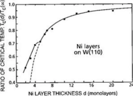
Figure 1.10: Thickness dependence of the critical point, referred to the bulk value

Tc(∞), in Ni(111) grown on top of W(110). Dashed line is a theoretical fit (see

reference for more details). Image from [50].

where J is the exchange integral, KB the Boltzmann’s constant and, most

important, ν the number of coordinated atoms. Hence it is now evident that the critical point depends upon the dimensionality of the system and particularly for surfaces and thin films, where a lower coordination occurs, it is expected to be lower than the bulk value. Such a behavior has been experimentally verified. In figure 1.10 the Curie temperature for a Ni layer grown on top of a W(110) substrate measured via magnetic resonance is reported as a function of the layer thickness [50]. More recently, magnetic dichroism in X-ray absorption spectroscopy has been largely employed in the determination of the critical temperature in ferromagnetic as well as antiferromagnetic thin films. Particularly for antiferromagnets, like NiO, because of its macroscopic magnetisation is null at any temperature, very few techniques are useful. In such a case X-ray Magnetic Linear Dichroism (XMLD), sensitive to the square of the magnetisation, ⟨M2⟩, has proved a useful tool to determine the N´eel temperature for films of diﬀerent thickness as reported in figure 1.11. The magnetic information is carried out by the so called L2 ratio which represents the asymmetry in the lineshape of the

L2 absorption edge due to the exchange interaction (as will be discussed in

section 4.1.3): upon increasing the temperature this asymmetry is reduced down to a constant value once the N´eel temperature is exceeded. Figure 1.11b puts in evidence also the role of the substrate in aﬀecting the magnetic properties of thin films: in its bottom panel the same 3 ML-thick film of NiO shows a TN = 390 K when grown on a silver substrate, while TN < 40 K in

the case of a MgO substrate [51, 52].

(42)

32

(a) Temperature and thickness dependence of the intensity ratio in Ni L2-XAS doublet in

NiO(100). A N´eel temperature of TN = 295,

430 and 470 K for 5, 10 and 20ML-thick films respectively have been found. From [51]

(b) Temperature dependence of the intensity ratio in Ni L2-XAS

dou-blet for 30 ML NiO(100)/Ag(100) (top) and 3 ML NiO(100)/Ag(100) (bottom, red) versus 3 ML NiO(100)/MgO(100) (bottom, blue). From [52].