Technical Report CoSBi 14/2007
Towards the integration of computational
systems biology and high-throughput data: a
way to support dierential analysis of
microarray gene expression data
Nicola Segata
DISI, University of Trento
[email protected]
Enrico Blanzieri
DISI, University of Trento
[email protected]
Corrado Priami
CoSBi
and
DISI, University of Trento
[email protected]
This is the preliminary version of a paper that will appear in
Journal of Integrative Bioinformatics, 5(1):87-103, 2008
Abstract. The paradigmatic shift occurred in biology that led first to high-throughput experimental techniques and later to computational sys-tems biology must be applied also to the analysis paradigm of the relation between local models and data to obtain an effective prediction frame-work. In this work we show that the new relation between systems biol-ogy models and high-throughput data permits new integrations on the systemic scale like the use of in silico predictions to support the mining of gene expression datasets. We introduce a unifying notational frame-work in which we propose two applications concerning the use of system level models to support the differential analysis of microarray expression data. The approach is tested with a specific microarray experiment on the phosphate system in Saccharomyces cerevisiae and a computational model of the PHO pathway that supports the systems biology concepts.
1
Introduction
Computational modelling of biological phenomena is motivated by the need of abstract representations of complex biochemical systems with the possibility to quantitatively reproduce and predict their behaviour. The sophistication reached by computers and programming languages permits one to effectively simulate the models allowing in silico predictions at the level of intricate metabolic and sig-nalling pathways like in [5][6]. Even though the complexity of these models can be very high, they still describe local aspects of biochemical systems. Recently, a paradigmatic shift in the dimensions and complexity of the models is occurring as consequence of the introduction of modelling paradigms that natively handle high parallelism and incremental model construction [14][12]. An example of ap-plication of these new paradigms is the PHO pathway model presented in [16] in which we model and simulate the phosphate systems in Saccharomyces
cere-visiae with the stochastic π-calculus, a language that support compositionality
(the ability of building models incrementally). In this scenario the models can reach the systems biology level (as schematized with the compositional model of Figure 1). Although the system level modelling of simple microorganisms is still more theoretical than effective, the potentialities of the in silico approach in this context are extremely promising for the biological community.
The systems biology concept [8] that is now becoming crucial in the com-putational modelling field, received the definitive incentive with the success, especially in certain areas, of the “globalists” over the “localists” [7]. The main factor for the shift from the local study of biochemical pathway to the genomic scale analysis of interaction networks was the developing of massively-parallel and high-throughput techniques [9] which made available a huge amount of unstructured gene-specific or protein-specific data. One of the more important high-throughput techniques is the microarray technology, used for example in [3] to detect the genes related to the phosphate accumulation and polyphosphate metabolism in Saccharomyces cerevisiae. The identification of genes that show significant changes in expression associated with experimental variables of inter-est on a microarray is called differential analysis of gene expression data [4][13]
and it is not a trivial task because the high-throughput datasets are large, ex-tremely noisy and subject to biological bias. The interpretation of the set of differentially expressed genes is a hot topic in research mainly because the typi-cal high cardinality of the set prevents the functional profiling and the validation of each gene singularly. Some authors addressed the problem through literature profiling [2] or Gene Ontology-based tools [11].
Exp1 Data1 M1, P1 Exp2 Data2 M2, P2 Exp3 Data3 M3, P3 Expi Datai Mi, Pi Expn Datan Mn, Pn Compositional model
High throughput dataset High throughput experiment
Fig. 1: Integration between local models and data and between systemic model and high-throughput data. Each local model Mxwith the corresponding parameters Pxcan
be integrated with classical relations of tuning and validation with specific data (Datax)
retrieved by proper experiments (Expx). The systems biology model, built composing
the local sub-models, have new possibilities of integration with high-throughput data. The + symbol stands for the abstract compositional operator of the models.
Regardless to the dimensionality, a model can assume a biological valence only if there are experimental data for the same biological aspect. Typical re-lations between data and models are parameter estimation, model validation and output data interpretation. When the biological description is not on a system level, there is a one-to-one relation between a local model and the pos-sibly available data that permits in silico simulations and thus biological pre-dictions (schematized in Figure 1 with the double arrows between each local model and each dataset derived from specific experiments). However, data from of high-throughput techniques are not suitable for tune and validate local path-way models because of the genomic scale and the uncertainty of the datasets. With the introduction of computational systems biology, new analysis paradigms of the relation between systems biology models and high-throughput can be ex-plored (the big double arrow in Figure 1). For example, the definition of these new paradigms can highlight the relation between the PHO pathway model [16] and the genic expression data on the phosphate metabolism in Saccharomyces
cerevisiae [3]. Therefore, as the shift from biology to systems biology needed a
how to handle some critical aspects like the uncertainty and dimensionality of the high-throughput techniques and the computational weight of the models that makes too many replicas of in silico predictions heavy.
In this work, we show that the expression datasets obtained with in
sil-ico simulations of system level models can support the differential microarray
analysis. This approach is possible assuming to have a reasonable large model built in a compositional way, thus permitting the independent validation of each pathway with biological data and it is complementary to other knowledge-based mining methods. We define a unifying notational framework for the experimental high-throughput data and in silico high-throughput expression values obtained with a computational model. The model indirectly reflects the state of the art of the biological knowledge, so the framework allows the biological information to be included in the process of microarray expression mining with the prediction potentialities of the systems biology models. The first application we propose in the framework aims to remove from the set of regulated genes those genes that the model predicts as normal to be regulated in the specific conditions. In this way the experimenter can focus only on the genes with really new biological in-formation. We effectively test the introduced approach and the first application to the microarray experiment of [3] using the PHO pathway model [16]. Even if this model is not on the genomic scale, it highlights the utility of the methods and confirms that, as the models scale up to the system level, our approach can give a systematic support to the the analysis of regulated genes in microarray experiments. The second application tackles the problem of the genes that are regulated by dependent and non directly controllable conditions that crowd the set of differentially expressed genes, possibly hiding genes regulated only by the direct and desired experimental conditions. This application is based on the in
silico prediction of the effects on gene expression of the dependent variables only.
The paper is organized as follows: Section 2 introduces the unifying notational framework for microarray and in silico gene expression experiments. Section 3 focuses on the specialization of the framework for microarray differential analysis proposing some measures for quantifying the level and the precision of the inte-gration. Section 4 describes the two specific application based on the framework and in Section 5 we discuss the possibility of developing general software tools in this context. The running example based on the microarray work of [3] and the PHO pathway model [16] is discussed step by step in the sections.
2
A unifying notational framework
We define a framework to formally specify the microarray experiments and the model-based estimation of gene expression in order to allow integrations of the two approaches. We focus on Affymetrix oligonucleotide chips [10] as far as the microarray technology is concerned, even though the framework can be adapted to cDNA chips. The cDNA chips, in fact, can be modelled as the combinations of two Affymetrix chips reflecting the expression of Cy3- and Cy5-labeled probes, like in the case of the microarray experiment of the running example.
2.1 The microarray experiments
An Affymetrix microarray experiment consists in the absolute quantification of the expression profiles of a set of genes. The parameters of a microarray experiment are essentially the controlled independent variables with their levels, and the measured dependent variables. Formally, the parameters are
qµA= (GµA, C, M, P ) (1)
where:
GµA is the set of genes that are spotted on the microarray1.
C ={(V1, l1), (V2, l2), . . . , (Vk−1, lk−1), (Vk, lk)} is the set of k different
condi-tions applied on the chip. A condition Ci with 1 ≤ i ≤ k is a pair (Vi, li)
where Vi is an independent variable controlled by the experimenter and li∈ R is a real value assigned to the variable. Hereafter, we assume that the
set of k independent variables V = {V1, V2, . . . , Vk−1, Vk} can be retrieved
from the experiment with the function IV (qµA) = V .
M ={(Vk+1, mk+1), (Vk+2, mk+2), . . . , (Vn−1, mn−1), (Vn, mn)} is the set of n−
k different dependent measured parameters of the chip. A dependent
mea-sured parameters Mi with k + 1 ≤ i ≤ n is a pair (Vi, mi) where Vi is
a dependent measured variable and mi ∈ R is the real value assigned to
the variable. Hereafter we assume that the set of dependent variables VD= {Vk+1, Vk+2, . . . , Vn−1, Vn} can be retrieved with the function DV (qµA) = VD and that V ∩ VD= ∅.
P represents the information regarding the experiment. It should contains the parameters that are not variable and that are sufficient to reproduce the experiment in a rigorous way. For instance, P may contain the sample used, the extract preparation and labeling, the procedure and the parameters for the hybridization and the environment and instruments information. In gen-eral it can contains all the information of the MIAME exchange standard [1] not handled by the other defined parameters.
With this conventions, the cDNA chip used in [3] (FODB are the initials of the authors) for the expression profiling between low and high phosphate conditions can be represented with the two following Affymetrix microarray experiments
F ODBµA,Cy3= (GF ODBµA ,{Pi, 0.2mM}, ∅, PF ODB) F ODBµA,Cy5= (GF ODB
µA ,{Pi, 10mM}, ∅, PF ODB)
Where GF ODB
µA is the set of genes considered in the experiment (approximatively
6400 distinct DNA sequences, available in the additional materials of [3]), Pi is
the phosphate concentration, and PF ODBcontains an exhaustive qualitative and
quantitative description of the experimental parameters that allows experimen-tal reproduction. The only experimenexperimen-tal independent variable is the phosphate
1 Note that it is not always trivial to associate a gene to each spot on the microarray
concentration IV (F ODBµA,Cy3) = IV (F ODBµA,Cy5) = Piwhich assumes two
different values in the two chips. The work does not measure any dependent variables (so DV (qµA) = ∅).
For a specific microarray experiment we can define a function reflecting the experimental procedure (which is as standard as possible) that promotes the biochemical reactions on the chip and results in the values of absolute expres-sion detected by the experimental instruments. This function for a microarray experiment qµA = (GµA, C, M, P ) has the form
ExprqµA : G &→ R (2)
ExprqµA associates to a gene g ∈ GµA a real value reflecting its expression.
All the genes spotted on the microarray with the corresponding expression values are included in a dataset, denoted as EqµA and defined as
EqµA = {(g, ExprqµA(g)) | g ∈ GµA} (3)
The dataset of the microarray experiment of our example is EF ODBµA and
is available in the additional materials of [3] with the relative quantification between F ODBµA,Cy3 and F ODBµA,Cy5 since a cDNA technology is used.
2.2 The in silico model-based simulation of expression experiments Here we propose how to simulate in silico an experiment to obtain a dataset of expression profiles. The model can be viewed as a set of metabolic and signalling pathways interacting each others. In particular, the prerequisites for a model to be suitable in this context are mainly three:
– The model must consider the gene transcription and allow the quantification of gene expression during the simulations.
– The model must have a genomic scale; it is not necessary to have a com-prehensive model of all the genes of the cell, but the number of considered genes must be comparable to number of genes spotted on a microarray chip. – The model must allow in silico experiments that accepts as inputs the envi-ronment conditions (like concentrations of the nutrients, temperature, pH, etc.) as independent variables controlled by the experimenter.
The PHO model we use to test the framework, matches the first and the last conditions. The genomic scale, instead, is not respected, and so the model is not suitable for real large-scale microarray mining, but it can still test the usefulness and quality of the approach. Moreover, the used modelling language support the incremental development, and so the model can be extended to other pathways influencing more genes.
In the definition of the microarray experiment we have the controllable con-ditions, the dependent variables and the parameters; the intuition is that they match the input requirements of an in silico simulation of a sufficient large sub-set of the biological network of a cell. So, similarly to the microarray experiment
we can give the following definition of the parameters of a model-based in silico expression experiment:
qm= (Gm, C, M, P ) (4)
where C, M and P are the conditions, the measured parameters and the exper-imental information as defined for qµA, while Gm is the set of genes for which
the model is able to estimate the expression profile.
The simulated expression experiments described in [16] (SBP are the ini-tials of the authors, lp and hp are the label denoting respectively low and high phosphate conditions) of the reference microarray work [3], are
SBPm,lp= (GSBPm ,{Pi, 0.2mM}, ∅, PSBP) SBPm,hp= (GSBP
m ,{Pi, 10mM}, ∅, PSBP)
with the same definition given for F ODBµA,Cy3 and F ODBµA,Cy5 except for PSBP which is the in silico correspondent of PF ODBand GSBP
m which contains
very few genes with respect to GF ODB
µA since the used model has not a genomic
scale. In particular
GSBPm = {PHO2,PHO4,PHO81,PHO5} (5)
The expression of a gene can be seen as the result of a particular instance of the model that is simulated with the particular inputs. So, with a conceptual analogous of the microarray expression function, for every qm there exists an
intensionally defined function that associates a real value to each gene as follows
Exprqm: G &→ R (6)
Exprqm reflects the simulated biochemical reactions occurring in a living cell,
while ExprqµA reflects the biochemical reactions occurring in the microarray
experiment preparation. ExprqµA and Exprqm can be seen as in silico and
high-throughput approximations of the real function that results in the gene expres-sion regulation in a living cell. The corresponding dataset for Exprqm is
Eqm = {(g, Exprqm(g)) | g ∈ Gm} (7)
The datasets of the in silico PHO pathway experiment are EqSBP
m,lp and EqSBPm,hp.
3
Differential analysis of microarray gene expression data
The main objective in gene expression analysis is the detection of the genes that are differentially expressed (or regulated) between two biological samples with some experimental differences. In differential analysis the classification of the genes is made with complex statistical techniques that analyse the entire distribution of gene expressions [4][17].We define the following microarray experiments:
q1
µA= (GµA, C1, M1, P ) q2
µA= (GµA, C2, M2, P )
with IV (qµA1 ) = IV (qµA2 ) and DV (q1
µA) = DV (qµA2 )
q1
µA and qµA2 can differ for definition only in the quantification of the dependent
and independent measured variables.
The set RµA⊆ GµArepresents the genes that are regulated between the two
microarray experiments q1
µA and qµA2 which reflect the differences between C1
and C2 and between M1 and M2. In the formalism defined for the microarray experiments this set can be detected by a class of functions called δµA that, in
general, takes two datasets and returns the genes that are regulated2:
RµA= δµA(Eq1µA, EqµA2 ) (9)
In our microarray reference experiment [3], the δµA function is based on the
two-fold derepression ratio, and the resulting set of regulated genes RF ODB µA ,
calculated as δµA(EF ODBµA,Cy3, EF ODBµA,Cy5), is
RF ODB
µA = {PHO5,PHO11,PHO12,PHO8,PHO84,PHO89,PHO86,PHO81,SPL2,PHM1,
PHM2,PHM3,PHM4,PHM5,PHM6,PHM7,PHM8,HOR2,CTF19,HIS1} (10) The same procedure can be applied to the expressions retrieved from the in
silico simulations. The experiments are defined maintaining the same conditions
and so the same dependent variables of the microarray experiment:
q1 m= (Gm, C1, M1, P ) q2 m= (Gm, C2, M2, P ) with IV (qm1) = IV (qm2) and DV (q1 m) = DV (q2m) (11) On q1
mand qm2 we can now apply the classification function δm which is, in
general, different from δµA because the assumptions on the distribution of the
expression dataset of a microarray and of in silico experiment can differ. The set of regulated genes with the in silico approach is denoted with Rm⊆ Gmand
computed with a δm function :
Rm= δm(Eq1
m, Eq2m) (12)
This formula, in the case of the PHO pathway model, is RSBP
m = δm(EqSBP m,lp, Eq
SBP m,hp)
and, via the computational simulations, gives the following set
RSBPm = {PHO81,PHO5} (13)
In ideal conditions we should have RµA = Rm (and Gm = GµA), but in
a scenario where all kind of systematic and random errors can occur the GµA, Gm, RµAand Rmsets are all potentially different. We further discuss the subsets
of RµA which is the set of genes we want to “clean”, distinguishing the cases Gm⊆ GµA, Gm≡ GµA and GµA⊆ Gm. Since the microarray chips can handle
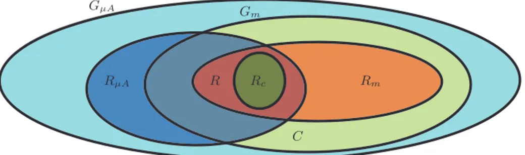
almost the whole genome while the computational models are still far from it (as in our case), we focus on the first case represented in Figure 2:
2 The δ
µA as used here accepts two expression datasets, but it can be generalised to
GµA RµA Gm Rm R Rc C
Fig. 2: Representation of the possible intersections between GµA(the set of genes with
a correspondent spot on the microarray), Gm(the set of genes considered in the model),
RµA(the set of regulated genes in the microarray) and Rm(the set of regulated genes
in the in silico experiment) assuming Gm⊆ GµA.
RµA\ Gm contains the microarray regulated genes which are not considered in
the computational model. The genes in this set are those whose investigation can potentially increase the biological knowledge and improve the model. R = RµA∩ Rm represents the set of genes that are regulated in both approaches.
Rc ⊆ R contains, for definition, the genes of the model that are regulated in a
consistent way with respect to the regulations detected by the microarray:
Rc = ! g∈ RµA∩ Rm " " " Exprq 1 µA(g) ExprqµA2 (g) * Exprq1 m(g) Exprq2 m(g) # (14) The expression comparison operator (*) is not precisely defined since dif-ferent levels of consistency can be considered. The most restrictive is the =, while the less restrictive is an operator that evaluates to true if the gene is over or under expressed (expression ratio greater or less than 1) in both approaches, but other intermediate operators can be defined. Also the com-parison of the expression ratios is not the only comcom-parison technique [17]. The set of the genes that are regulated consistently (with a comparison based on the over- or under-expressed condition) between RF ODB
µA and RSBPm of our
running example is
RP HOc = {PHO81,PHO5} (15)
(RµA∩ Gm) \ R contains the genes regulated in the microarray but not in the
in silico simulations. The mismatch can be due to errors, or to the lack of
biological information on which the model is constructed. Other meaningful sets are:
C = (GµA∩ Gm) \ (RµA∪ Rm) the set of genes that are constitutive (i.e. not
regulated) in both microarray and in silico experiments. In the running example we have that CP HO= {PHO2,PHO4}
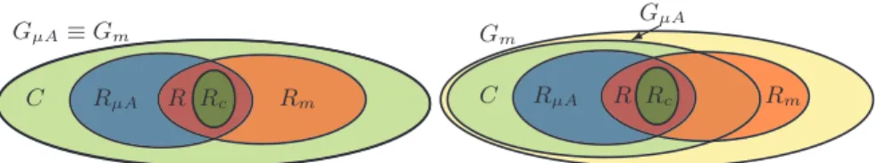
GµA≡ Gm RµA R Rc Rm C GµA ! ! " Gm RµA R Rc Rm C
Fig. 3: Representation of GµA, Gm, RµAand Rmassuming Gm≡ GµAand GµA⊆ Gm.
The cases Gm ≡ GµA and GµA ⊆ Gm are represented in Figure 3; the main
differences with the Gm ⊆ GµA case are that RµA\ Gm = ∅ and that in the GµA ⊆ Gm case there is the Rm\ GµA set of the genes considered in the
com-putational model but not on the microarray chip. 3.1 Accuracy and coverage measures
From a methodological point of view, for the genes in Rc and in C the
mod-elling approach is consistent with the microarray one, while the genes in R \ Rc,
(RµA∩ Gm) \ R and (Rm∩ GµA) \ R represent an incongruence between the
approaches. With these sets we can formally define the accuracy of the combi-nation of computational modelling (and indirectly of the biological knowledge) and of the microarray information in the following way:
A = |Rc| + |C| |GµA∩ Gm|× 100
(16) Another measure of the quality of the framework applied to specific cases reflects the gene coverage level of the model with respect to the microarray chip. This measure is called chip coverage and can be defined as follows:
Cov =|GµA∩ Gm| |GµA| × 100
(17) It is an a priori quantification of the percentage of the genes in the microarray chip that are also considered in the model. However, a low chip coverage does not implies that the approach is useless because the microarray regulated genes can be highly covered by the model even if the chip is poorly covered. So another coverage measure, that we call experimental coverage (Cove), is introduced:
Cove= |RµA∩ Gm| |RµA| × 100
(18) This value can be calculated only when both the microarray and the in silico experiment are performed and it is referred only to a single experiment, but it is a more accurate evaluation of the experimental quality. Moreover, minimizing the chip coverage after maximizing the experimental coverage, gives the same results of a complete chip coverage, but it requires a much lower computational effort to perform the in silico experiments. On the other hand a complete chip coverage
permits to use the same computational model for all the possible experiment with that chip. In any case, the coverage and the accuracy must be considered together for evaluating the overall quality of the approach for a performed experiment.
Observing on the running example that |RP HO
c | = 2, |CP HO| = 2, |GF ODBµA ∩ GSBP
m | = |GSBPm | = 4, |GF ODBµA | = 6400, |RF ODBµA | = 20 and |RF ODBµA ∩ GSBPm | =
2, the introduced measure are:
AP HO= 100% CovP HO= 0, 0625% CovP HOe = 10%
This means that the model predicts the expression profiles consistently with the microarray experiment, but the coverage is very low as we expected since the model is local. The relatively high experimental coverage means that the model fits at least partially the pathways whose genes are interested in the regulation.
4
Applications in microarray differential analysis
The set of genes detected with the microarray differential analysis whose reg-ulation is in relation with a specific condition, can be very large and so hard to analyse. The applications we propose here are based on the described frame-work and are intended to be applied on the set of differentially expressed genes in order to detect the most informative genes before further analysis.
4.1 Removing the genes regulated in the in silico predictions The set of regulated genes can include many genes that are already indirectly known to be related with the conditions of the analysis. The removing of these genes allows the biologist to focus only on the really unknown genes that can thus have more new biological information. The idea is to use computational models, built on the current biological knowledge, to predict the genes that will be regulated in a specific microarray experiment and remove them from the microarray experimental results.
So, the aim of this application is to filter out from the regulated genes of the microarray experiment (RµA), those genes that the model suggests to be
regulated (Rm). We would remove directly the genes in Rm from the genes in RµA. In other words the set of really interesting genes Rint would be:
Rint= RµA\ Rm (19)
In presence of errors and approximations, the definition of the interesting reg-ulated genes Rint as RµA\ Rm is no more acceptable mainly because the
un-certainty on Rm. We need a more robust definition of the set of genes that can
be safely removed from the microarray regulated ones. So instead of subtracting from RµA the Rm set, we subtract the genes that are regulated in a consistent
way in both approaches, i.e. the Rc set as defined in (14). So:
Returning to the running example, this definition is RP HO
int = RF ODBµA \RP HOc
where the RF ODB
µA and RP HOc sets are computed and shown respectively in (10)
and (15). The resulting set of really interesting genes is
RP HO
int = {PHO11,PHO12,PHO8,PHO84,PHO89,PHO86,SPL2,PHM1,PHM2,PHM3,
PHM4,PHM5,PHM6,PHM7,PHM8,HOR2,CTF19,HIS1} (21) Our application has filtered out from the set of regulated genes of the reference microarray experiment [3] two genes (PHO5 andPHO81) predicted by the
com-putational model [16]. So we have reduced the number of genes that represent new biological information suggesting that this application is useful.
The genes considered in the model are only 4, and the two that have been removed from RP HO
int are those that the model predicts sensitive to different
phosphate metabolism. So, as the accuracy measure (AP HO = 100%) suggests,
the model predictions are in this case the more desirable ones with respect to the very low coverage. We can conclude that this application can be a helpful tool for a biologists, especially in the cases where the microarray experiment detects an high number of regulated genes and the computational model has a reasonable good experimental coverage in addition to the accuracy.
4.2 Removing the genes regulated by the non controlled variables The definition of the microarray experiment includes the notion of controlled conditions and dependent not-directly controlled variables. Obviously the ef-fects of the dependent variables in terms of regulated genes cannot be detected in isolation or separated from the independent variable effects through the mi-croarray experiment. Since biologists are interested in the genes regulated only by the directly controlled conditions, the idea of this application is to estimate
in silico the genes that are regulated because of the dependent variables in order
to remove them from the set of microarray regulated genes. Note that the values of the dependent variables included in the specification of the in silico gene ex-pression experiments are those measured on the microarray experiment. Since, as discussed, the microarray experiment of [3] does not provide any dependent variables, we cannot test this conceptual application with our running example.
Consider the following three microarray experiments3:
qµA = (G, C, M, P ) qcntr
µA = (G, Ccntr, Mcntr, P ) qµAh = (G, C, Mcntr, P )
with IV (qµA) = IV (qµAcntr) = IV (qhµA) and DV (qµA) = DV (qµAcntr) = DV (qhµA).
The first two chips are a microarray experiment (qµA) and the relative control
chip (qcntr
µA ), while the third (qhµA) is a hypothetical variation of the microarray
chips in which the actual values of dependent variable are replaced with the control ones. Notice that the qh
µA experiment cannot be really performed since 3 In this subsection we assume that the set of genes spotted on the microarray and
the set of genes considered in the model are identical, without loosing generality. Formally: G = GµA≡ Gm
the values of the independent variables C force the values of the dependent controlled variables to be M and not Mcntr. Suppose to apply a δ
µAfunction in
the following way:
RµA= δµA(EqµA, EqµAcntr) R
V µA= δµA(Eqh µA, Eq cntr µA ) R VD
µA= δµA(EqµA, EqµAh )
RµA is the standard set of genes that are regulated because of the differences
between levels of the independent a dependent variables between the two chips,
RV
µA contains the genes that are regulated only by the independent variables
(since qh
µA and qcntrµA have the same values of dependent variables Mcntr), and RVD
µA represents the genes that are regulated only by the dependent variables
(since qµA and qhµA have the same values of the independent variables C). RVµA
is the set of genes that the experimenter would have because it is not influenced by the dependent variables, but it is not possible to obtain because the qh
µA chip
is only hypothetical.
Under the assumption that the sets of genes regulated by the dependent and independent variables are disjoint, RV
µA could be estimated subtracting from RµA the genes that are regulated because of the dependent variable RVD
µA. So
RVµA= RµA\ RVµAD (22)
but also RVD
µA is not possible to obtain, since it needs the hypothetical qhµA chip.
However, in this framework we have the possibility to estimate expression experiments with the computational model. In particular, all the following ex-periments can be performed in silico:
qm= (G, C, M, P ) qcntr
m = (G, Ccntr, Mcntr, P ) qmh = (G, C, Mcntr, P )
With these in silico experiments it is possible to detect the gene regulated only by the independent (RV
m) and only by the dependent variables (RVmD): RV m= δm(Eqh m, Eqmcntr) R VD m = δm(Eqm, Eqh m)
The direct approximation of RV
µAwith RVmis useless because in this way we rely
only on the model, loosing the information of the microarray experiment. The idea for integrate the microarray and the in silico data consists in filter-ing out from the set of microarray regulated genes those genes that are regulated because of the dependent variables, substituting RVD
µA with RVmD in (22)
RVµA* RµA\ RVmD (23)
If a gene is regulated both because of the independent and because of the depen-dent variables, the estimation of RV
µA will not include that gene. For this reason
is necessary to assure that V and VDregulate two different set of genes meaning
Definition 1. V and VDare disjoint with respect to the gene regulation, or sim-ply, ge-disjoint, if and only if for every possible values associated to the variables the following holds: RV
µA∩ R VD
µA = ∅ ∧ RVm∩ RVmD = ∅
This definition is too restrictive because it is impossible to directly obtain RV µA
and RVD
µA. However, the theoretical definition can be made less strict for an
effective application if we have an high accuracy and a good confidence in the quantitative estimation of gene expression of the model.
Definition 2. V and VD are ge-disjoint, if and only if for every possible values associated to them the following holds: RV
m∩ RVmD = ∅
The complete definition for removing from the set of regulated genes of a mi-croarray, the genes that are regulated only by the dependent variables, is
RV
µA* RµA\ RVmD if RVm∩ RVmD = ∅ (24)
If V and VD are not ge-disjoint (or if it is not possible to show it), we can
partition VD in two subsets VD", VD""⊂ VD with VD" ∩ VD""= ∅ and VD" ∪ VD""= VD
such that V"
D and V are ge-disjoint. At this point we can still remove some genes
from RµA, and precisely the genes that are regulated because of VD".
So in the cases where it is possible to show that the set of independent variables (or a subset) are ge-disjoint from the set (or from a subset) of the dependent measured variables, we can remove all (or some of) the genes that are not directly regulated by the experimental conditions.
5
From a conceptual to a software framework
Our notational framework can be a guide for the development of software tools for supporting analyses that combine the two fields of the microarray technology and the system level modelling and simulation of biological networks. While for the first a lot of bioinformatics tools have been developed for every aspect of the technology, the second still needs research in order to make the development and the simulation of systems biology models effective.
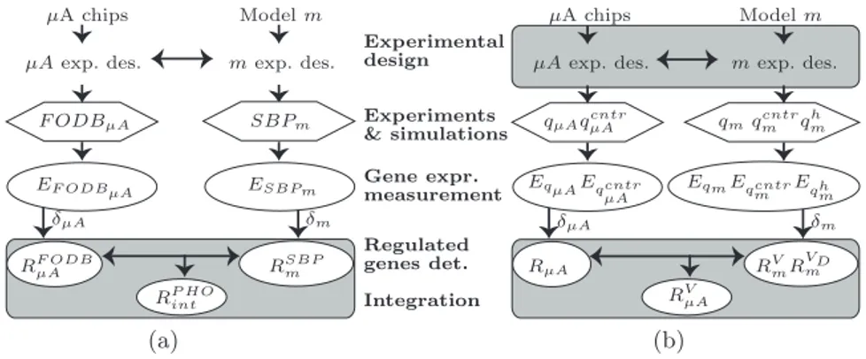
Our conceptual framework assumes to have a computational model and mi-croarray chips and can actively act on different phases: the experimental con-ditions and design, the expression profiling, the regulated genes detection and the integration of regulated genes belonging to the two approaches. The first application (Figure 4.a) concerns only the manipulation of the regulated genes belonging to microarray and in silico experiments designed with the same con-ditions, while the second (Figure 4.b) interests also the design, requiring some experiments with particular settings of the dependent and independent condi-tions. Other applications can regards also the other phases. Regardless of the number of phases interested in the specific case, each phase requires formal and software tools to allow real implementations of applications in the framework. We discuss the availability of implemented software or formal specification for each phase:
(a) (b)
µA chips Model m µA exp. des. m exp. des.
F ODBµA SBPm EF ODBµA ESBPm RF ODB µA RSBPm RP HOint δµA δm
µA chips Model m µA exp. des. m exp. des.
qµAqcntrµA qmq cntr m q h m EqµAEqcntr µA EqmEqcntr m Eqhm RµA RV mRVDm RV µA δµA δm Experimental design Experiments & simulations Gene expr. measurement Regulated genes det. Integration
Fig. 4: These schemes highlight the modules interested by the application for removing the genes regulated in the in silico predictions (a) and by the application for removing the genes regulated by the non controlled variables (b).
Experimental design Approfondite studies have been done to make microar-ray experiments maximally informative, given the effort and the resources [18] [19]. In this work we assume that an in silico simulated microarray exper-iment has the same abstract behaviour of the real one; for this reason all the designs reported in literature can be applied also to the simulated case. However, some improvements can be done relying on the fact that once the model is developed the simulation cost is much lower than the microarray experimental one. Moreover some hybrid designs are possible integrating in the same design simulated and real microarray experiments.
Experiments and simulations The microarray experimental procedure has reached a good level of standardization [1]. Instead, the possible sources of variability in the computational simulation rely on model errors and ap-proximations in the simulation algorithm; however, both problems regard in general the computational modelling of biological systems, while the simu-lation procedure is intrinsically standard.
Gene expression measurement The output of a microarray experiment is obtained with the optical scan of the array and the analysis of the result-ing image. Software tools for this operation are available. Both microarray output after scanning and in silico expression results, needs normalization procedures to make meaningful comparisons of expression levels. For mi-croarray experiments, statistical methods and software are available [15], while for the in silico simulations specific normalization procedures must be developed because the distribution of the expression can a priori be different from the microarray ones. Since in silico microarray outputs are not avail-able, more precise discussions cannot be done, but it is reasonable to adapt some microarray techniques with specific parameters and thresholds. Regulated genes detection Statistical techniques for the δµA like [17] are
available and implemented. δm, instead, was never developed, but the
simulations are not affected by the random experimental error and by ap-proximation in the optical scanning of the chip and so they are less noisy. Integration of regulated gene sets The integration of the set of regulated
genes are normal operations on sets and can thus be easily implemented.
6
Conclusions
The traditional use of biological models concerns the parameters estimation and the qualitative and quantitative description of not directly observable and high level behaviours. In this work we propose to use systems biology models to sup-port analysis of high-throughput data; it can be seen as a way to compare the current biological knowledge with new genomic experiments. The comparison aims to discover unknown aspects of complex and wide biological networks al-lowing to focus further investigations only on that very specific subnetworks. The overall procedure is somehow recursive since the new discoveries reached starting from the model suggestions, permits improvements of the biological knowledge from which it is possible to construct more precise models.
The notation we introduced for the microarray experiments and the in
sil-ico simulations of gene expression was specialized in the context of differential
analysis. Then, we proposed two real applications of our conceptual framework with the purpose of supporting the mining of regulated genes detected with mi-croarray expression data. In the example on which we tested the work, we were able to remove two genes from the regulated genes of the microarray experiment, thus obtaining encouraging results and highlighting the utility of the approach, even if we used a local model. For this reason, as the model size grows reaching the systems biology level the impact of our approach on the high-throughput data interpretation can be very important.
References
1. A Brazma, P Hingamp, J Quackenbush, G Sherlock, P Spellman, C Stoeckert, J Aach, W Ansorge, CA Ball, HC Causton, et al. Minimum information about a microarray experiment (MIAME)-toward standards for microarray data. Nat
Genet, 29(4):365–71, 2001.
2. D Chaussabel and A Sher. Mining microarray expression data by literature profil-ing. Genome Biol, 3:research0055.1–0055.16, 2002.
3. GR Fink, N Ogawa, J DeRisi, and PO Brown. New Components of a System for Phosphate Accumulation and Polyphosphate Metabolism in Saccharomyces cerevisiae Revealed by Genomic Expression Analysis. Molecular Biology of the
Cell, 11(12):4309–4321, 2000.
4. GW Hatfield, SP Hung, and P Baldi. Differential analysis of dna microarray gene expression data. Mol Microbiol, 47(4):871877, 2003).
5. A Hoffmann, A Levchenko, ML Scott, and D Baltimore. The ikb-nf-kb signaling module: Temporal control and selective gene activation. Science, 298:1241–5, 2002.
6. CYF Huang and JE Ferrell. Ultrasensitivity in the mitogen-activated protein kinase cascade. Proc Natl Acad Sci, 93:10078–10083, 1996.
7. S Huang. Back to the biology in systems biology: What can we learn from biomolec-ular networks? Brief Funct Genomic Proteomic, 2(4):279–297, 2004.
8. H Kitano. System biology: A brief overview. Science, 295:1662–1664, 2002.
9. J Kononen, L Bubendorf, A Kallioniemi, M Barlund, P Schraml, S Leighton, J Torhorst, M Mihatsch, G Sauter, and O Kallioniemi. Tissue microarrays for high-throughput molecular profiling of tumor specimens. Nat Med, 4:844–7, 1998.
10. DJ Lockhart, H Dong, MC Byrne, MT Follettie, MV Gallo, MS Chee, M Mittmann, C Wang, M Kobayashi, H Horton, and EL Brown. Expression monitoring by hy-bridization to high-density oligonucleotide arrays. Nat Biotech, 14:1675–80, 1996.
11. P Pavlidis, J Qin, V Arango, JJ Mann, and E Sibille. Using the gene ontology for microarray data mining: A comparison of methods and application to age effects in human prefrontal cortex. Neurochem Res, 29(6):1213–1222, 2004.
12. M Peleg, I Yeh, and RB Altman. Modelling biological processes using workflow and petri net models. Bioinformatics, 18(6):825–837, 2002.
13. MS Pepe, GM Longton, GL Anderson, and M Schummer. Selecting differentially expressed genes from microarray experiments. Biometrix, 59(1):133–142, 2003.
14. C Priami and P Quaglia. Modelling the dynamics of biosystems. Brief Bioinform, 5(3):259–269, 2004.
15. J Quackenbush. Microarray data normalization and transformation. Nat Genet, 32:496–501, 2002.
16. N Segata, E Blanzieri, and C Priami. Stochastic π-calculus modelling of multisite phosphorylation based signaling: in silico analysis of the pho4 transcription factor and the pho pathway in saccharomyces cerevisiae. Technical Report TR-08-2007, Microsoft Research - University of Trento Centre for Computational and Systems Biology, 2007.
17. VG Tusher, R Tibshirani, and G Chu. Significance analysis of microarrays ap-plied to the ionizing radiation response. Proceedings of the National Academy of
Sciences, 98(9):5116–5121, 2001.
18. YH Yang and T Speed. Design issues for cDNA microarray experiments. Nat Rev
Genet, 3(8):579–588, 2002.
19. SO Zakharkin, K Kim, T Mehta, L Chen, S Barnes, KE Scheirer, RS Parrish, DB Allison, and GP Page. Sources of variation in Affymetrix microarray experi-ments. BMC Bioinformatics, 6(214):1471–2105, 2005.