2019
Publication Year
2021-02-16T15:24:08Z
Acceptance in OA@INAF
Analysis of full disc Ca II K spectroheliograms. II. Towards an accurate assessment
of long-term variations in plage areas
Title
CHATZISTERGOS, THEODOSIOS; ERMOLLI, Ilaria; Krivova, N. A.; Solanki, S. K.
Authors
10.1051/0004-6361/201834402
DOI
http://hdl.handle.net/20.500.12386/30410
Handle
ASTRONOMY & ASTROPHYSICS
Journal
625
Number
Astronomy & Astrophysics manuscript no. paper_segmentation_shg_18_arxiv ESO 2019c February 20, 2019
Analysis of full disc Ca II K spectroheliograms
II. Towards an accurate assessment of long-term variations in
plage areas
Theodosios Chatzistergos
1, 2, Ilaria Ermolli
1, Natalie A. Krivova
2, Sami K. Solanki
2, 31 INAF Osservatorio Astronomico di Roma, Via Frascati 33, 00078 Monte Porzio Catone, Italy
2 Max Planck Institute for Solar System Research, Justus-von-Liebig-weg 3, 37077 Göttingen, Germany 3 School of Space Research, Kyung Hee University, Yongin, Gyeonggi 446-701, Republic of Korea
ABSTRACT
Context. Reconstructions of past irradiance variations require suitable data on solar activity. The longest direct proxy is the sunspot number, and it has been most widely employed for this purpose. These data, however, only provide information on the surface magnetic field emerging in sunspots, while a suitable proxy of the evolution of the bright magnetic features, specifically faculae/plage and network, is missing. This information can potentially be extracted from the historical full-disc observations in the Ca II K line.
Aims. We use several historical archives of full-disc Ca II K observations to derive plage areas over more than a century. Employment of different datasets allows identification of systematic effects in the images, such as changes in instruments and procedures, as well as an assessment of the uncertainties in the results.
Methods. We have analysed over 100,000 historical images from 8 digitised photographic archives of the Arcetri, Ko-daikanal, McMath-Hulbert, Meudon, Mitaka, Mt Wilson, Schauinsland, and Wendelstein observatories, as well as one archive of modern observations from the Rome/PSPT. The analysed data cover the period 1893–2018. We first per-formed careful photometric calibration and compensation for the centre-to-limb variation, and then segmented the images to identify plage regions. This has been consistently applied to both historical and modern observations. Results. The plage series derived from different archives are generally in good agreement with each other. However, there are also clear deviations that most likely hint at intrinsic differences in the data and their digitisation. We showed that accurate image processing significantly reduces errors in the plage area estimates. Accurate photometric calibration also allows precise plage identification on images from different archives without the need to arbitrarily adjust the segmentation parameters. Finally, by comparing the plage area series from the various records, we found the conversion laws between them. This allowed us to produce a preliminary composite of the plage areas obtained from all the datasets studied here. This is a first step towards an accurate assessment of the long-term variation of plage regions.
Conclusions.
Key words. Sun: activity - Sun: photosphere - Sun: chromosphere - Sun: faculae, plages
1. Introduction
The Sun is the main external energy supplier to the Earth. The radiative energy from the Sun received per unit time and area at 1 AU is termed solar irradiance. Thus knowl-edge of solar irradiance is of crucial interest for climate studies (Haigh 2007; Gray et al. 2010; Ermolli et al. 2013; Solanki et al. 2013). Direct measurements of solar irradiance are available since 1978. They show that the total solar irra-diance (i.e., integrated over the entire solar spectrum) varies by about 0.1% in phase with the solar activity cycle, with sometimes even stronger fluctuations on the time scales of days. The records of direct measurements are however too short to investigate the solar impact on the complex cli-mate system of Earth properly. This calls for sufficiently long reconstructions of past irradiance variations.
Solar irradiance changes on time scales of days and longer are generally attributed to varying contributions
Send offprint requests to: Theodosios Chatzis-tergos e-mail: [email protected], [email protected]
of dark sunspots and bright facular and network regions (Shapiro et al. 2017). Models assuming that irradiance vari-ability is driven by the solar surface magnetic flux repro-duce over 90% of the measured total solar irradiance varia-tions (see e.g. Yeo et al. 2014, 2017, and references therein). The success of these models lent grounds to believe that re-constructions of past irradiance variability can give a real-istic picture of the Sun’s behaviour, provided there are suit-able data of solar magnetic activity. Direct measurements of the solar surface magnetic field exist only for roughly the same period as covered by irradiance measurements. To go further back in time, sunspot observations and isotope data are the typically employed proxies of solar magnetic activ-ity (e.g. Lean et al. 1995; Solanki & Fligge 1999; Wang et al. 2005; Steinhilber et al. 2009; Krivova et al. 2007, 2010; De-laygue & Bard 2011; Shapiro et al. 2011; Vieira et al. 2011; Dasi-Espuig et al. 2014, 2016; Cristaldi & Ermolli 2017; Wu et al. 2018). However, sunspot observations do not carry in-formation on faculae or the network, whereas isotope data trace primarily the open magnetic flux, which is only in-directly related to sunspot and facular fields. These
A&A proofs: manuscript no. paper_segmentation_shg_18_arxiv
tations can be overcome by combining observations taken in white-light and in the Ca II K spectral band to moni-tor sunspots and facular regions, respectively. Such obser-vations cover a period exceeding a century. Owing to the tight relationship between the Ca II K brightness and the non-sunspot magnetic field strength averaged over a pixel (Babcock & Babcock 1955; Skumanich et al. 1975; Schri-jver et al. 1989; Ortiz & Rast 2005; Loukitcheva et al. 2009; Pevtsov et al. 2016; Chatzistergos 2017; Kahil et al. 2017), the Ca II K observations can provide detailed information on the surface coverage by bright faculae and network re-gions (hereafter referred to as plage and network as Ca II K observations trace the chromosphere, where facular regions are called plage). This information should allow a signifi-cant improvement of long-term irradiance models, at least for the period of time that Ca II K data are available and possibly, indirectly, also for even longer periods of time.
In recent years, digitization of various archives (for a list of the available archives see Chatzistergos 2017) allowed starting extensive exploitation of historical Ca II K spec-troheliograms (SHG, e.g. Ribes & Mein 1985; Kariyappa & Pap 1996; Foukal 1996, 1998; Caccin et al. 1998; Worden et al. 1998; Zharkova et al. 2003; Lefebvre et al. 2005; Er-molli et al. 2009b,a; Tlatov et al. 2009; Bertello et al. 2010; Dorotovič et al. 2010; Sheeley et al. 2011; Priyal et al. 2014, 2017; Chatterjee et al. 2016, 2017). Overall, there are nu-merous published results from historical Ca II K images, which agree in some respects, but also show significant dif-ferences (see Ermolli et al. 2018). A critical aspect of most of these studies is, however, that they used photometrically uncalibrated images and did not analyse the possible sys-tematic changes of the quality of the images recorded by different observers over decades (see the discussion in Er-molli et al. 2009b). For example, simple visual examination of the available data shows that co-temporal observations from different series can diverge significantly due to the dif-ferences in spectral and spatial resolution of observations, stray-light, noise, calibration, and other instrumental and archival characteristics. Besides, diverse processing meth-ods were applied to the data from individual archives, thus hampering comparison of results from the various series. An accurate and homogeneous compilation of multiple datasets into a single series, critical for irradiance reconstructions and other studies, is thus a challenging task.
In Chatzistergos et al. (2018b) we introduced a novel approach to process the historical SHG observations and showed that it allows to perform the photometric calibra-tion and account for image artefacts with higher accuracy than obtained with other methods presented in the liter-ature. We also showed that the proposed method returns consistent results for images from different SHG archives (for examples see also Chatzistergos et al. 2018a).
In this paper we analyse carefully reduce and calibrate images from 8 historical and one modern archives of Ca II K observations to evaluate changes in plage area coverage from 1893 to 2018. Analysis of multiple archives helps us to assess systematic changes and sources of artefacts in the results derived from individual datasets.
The paper is organized as follows. In Sections 2 and 3 we describe the data analysed in our study and present a brief overview of the methods applied, respectively. Our re-sults for the plage areas are presented and compared with other published results in Section 4. In Section 5 we discuss the effects of photometric calibration and other processing
steps on the results, while in Section 6 we produce prelimi-nary composite series from the analysed data. In Section 7 we summarize the results of our study and draw our con-clusions.
2. Data
We consider full-disc Ca II K observations derived from the digitization of 8 historical SHG photographic archives and from the modern Rome/PSPT (Precision Solar Photo-metric Telescope). The latter data allow us to extend the time-series of plage areas derived from the historical obser-vations to the present day as well as to test the accuracy of our processing. The plage areas derived in this work are compared to other published records and to the sunspot area record compiled by Balmaceda et al. (2009)1
2.1. Full-disc Ca II K archives
The historical data analysed here are the digitized Ca II K full-disk SHG from the Arcetri (Ar), Kodaikanal (Ko), McMath-Hulbert (MM), Meudon (Me), Mitaka (Mi), Mount Wilson (MW), Schauinsland (Sc), and Wendelstein (WS) photographic archives. In brief, the observations were taken between 1893 and 2002 in the Ca II K line at λ = 3933.67 Å, with bandwidths ranging from 0.1 to 0.5 Å. The original photographic observations, which were mainly stored on photographic plates (MM observations are on sheet film, while Mi observations after 02/03/1960 are on 24x35 mm sheet film), were digitized by using different devices and methods. Information about the devices and settings that were used to convert the Ar, Ko, and MW data to digital images can be found in e.g. Ermolli et al. (2009b, and references therein), about Me in Mein & Ribes (1990), about Mi in Hanaoka (2013), and Sc and WS in Wöhl (2005). Table 1 summarizes key information about the different datasets used in this study.
Some series derive from combinations of observations taken at different sites, while some underwent multiple digi-tisations. For example, the Mi data were obtained at two different sites, Azabu (1917-1924) and Mitaka (1925-1974), and have been digitised three times, once with 8-bit depth and twice with 16-bit depth. Furthermore, the second digi-tisation includes only the data prior to 02/03/1960, while the third digitisation includes the data after 02/03/1960 as well as the first 10 observations of each year prior to 1961. In this work we analyse all the data from the third digi-tisation (2581 images) and use the data from the second digitisation for the missing dates (5943 images)2. The full-disc Ko data have been digitised two times, once with 8-bit depth (Makarov et al. 2004) and once with 16-bit depth (Priyal et al. 2014). Here we use the Ko data from the 8-bit digitisation. The MW data have been digitised two times, once with 8-bit depth (Foukal 1996) and once with 16-bit depth (Lefebvre et al. 2005). Here we use the 16-bit MW data. The Me data have been partially digitised at different periods with various set-ups. Some images have been digi-1 Available at http://www2.mps.mpg.de/projects/
sun-climate/data.html
2
The analysis presented by Chatzistergos (2017) and Chatzis-tergos et al. (2016, 2018b) was done with the data from the first 8-bit digitisation and the second digitisation for periods after and before 02/03/1960, respectively.
Chatzistergos et al.: Segmentation of Ca II K SHG
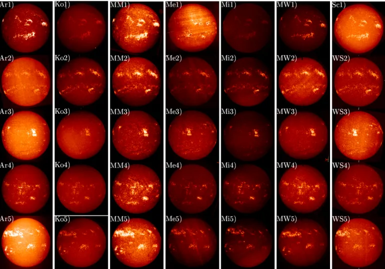
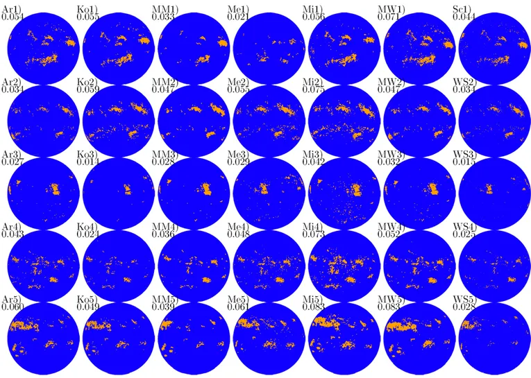
Fig. 1. Raw Ca II K density images from the Arcetri (Ar), Kodaikanal (Ko), McMath-Hulbert (MM), Meudon (Me), Mitaka (Mi), Mt Wilson (MW), Schauinsland (Sc), and Wendelstein (WS) observatories (Sc and WS are shown in a single column due to their low number of images). Each row shows observations from the different archives taken on roughly the same day, except for Me1. The dates of the observations are (from top to bottom): 09/12/1959 (17/11/1893 for Me), 01/03/1968 (29/02/1968 for Me), 01/08/1968 (30/07/1968 for Me and WS), 05/09/1968 (06/09/1968 for WS), and 18/03/1969 (17/03/1969 for Me and WS). All images are normalised to the range of values within the disc and are compensated for ephemeris.
tised multiple times. In these cases we kept only those from the most recent digitisation. The Sc, and WS data have only partially been digitised. Merely 18 and 452 plates out of 3131 and 4824 documented existing plates from the Sc and WS archives, respectively, were digitised. Most of the digitised images were stored in FITS files, the Mi data from the 3rd digitisation and most of the Sc and WS data were stored in TIFF files, while the MM and the remaining Sc and WS data were stored in JPG compressed files. The var-ious digitisations of the Me data were stored in GIF, TIFF, JPG, and FITS file formats. In a first step of our analysis all of the GIF, TIFF, and JPG files were converted to FITS files.
Calibration of the CCD employed for the digitisation was applied on the data from Ar observatory. MM, Sc, WS, and Mi data from the 3rd digitisation lack this processing step, while for Mi data from the earlier digitisations, as well as the Me, Ko, and MW data it is unclear whether this calibration was applied or not.
Figure 1 provides examples of images from each his-torical dataset taken on roughly the same five days, with the exception of panel Me1. The images were selected such that an observation from Sc or WS exists within an interval
of 2 days. This period is unfortunately restricted to 1959– 1969. Furthermore, panel Me1) shows the oldest available Ca II K observation from the analysed archives taken on 17/11/1893. The brightness scale is individually normal-ized to cover the values from the minimum (black) to the maximum (white) within the solar disc in each image. The figure shows, for instance different brightness properties, saturated regions in the Ar images (Ar1, Ar3, and Ar5), overexposed plage regions in MM observations (MM1 and MM5), or very bright small-scale artefacts in Mi observa-tions (Mi1). See Chatzistergos (2017) for a further discus-sion of problems affecting such data. Figure 1 is discussed in more detail in the Appendix A.
The modern observations (i.e. those taken with a CCD detector) analysed in this study were acquired with at the Meudon and the Rome observatories. Meudon observatory installed a CCD camera on 13/05/2002 and continued ob-servations with the same instrumental set-up, while storing data also on photographic plates up to 27/09/2002. The Rome observations were acquired with the Rome/PSPT, which is a 15 cm, low-scattered-light, refracting telescope designed for synoptic solar observations characterized by 0.1% pixel-to-pixel relative photometric precision (Coulter
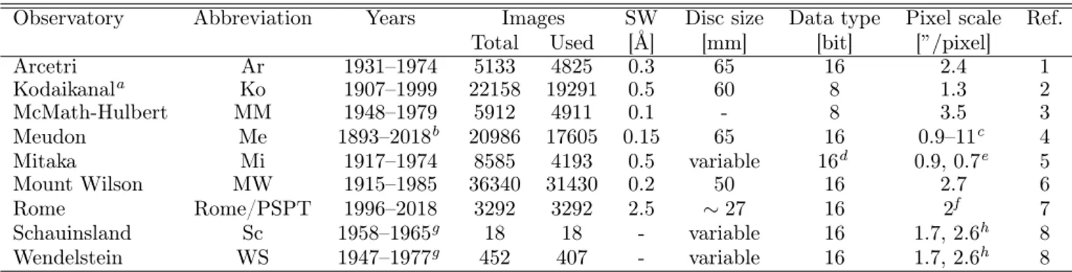
A&A proofs: manuscript no. paper_segmentation_shg_18_arxiv Table 1. List of Ca II K archives analysed in this study.
Observatory Abbreviation Years Images SW Disc size Data type Pixel scale Ref.
Total Used [Å] [mm] [bit] [”/pixel]
Arcetri Ar 1931–1974 5133 4825 0.3 65 16 2.4 1 Kodaikanala Ko 1907–1999 22158 19291 0.5 60 8 1.3 2 McMath-Hulbert MM 1948–1979 5912 4911 0.1 - 8 3.5 3 Meudon Me 1893–2018b 20986 17605 0.15 65 16 0.9–11c 4 Mitaka Mi 1917–1974 8585 4193 0.5 variable 16d 0.9, 0.7e 5 Mount Wilson MW 1915–1985 36340 31430 0.2 50 16 2.7 6 Rome Rome/PSPT 1996–2018 3292 3292 2.5 ∼ 27 16 2f 7 Schauinsland Sc 1958–1965g 18 18 - variable 16 1.7, 2.6h 8 Wendelstein WS 1947–1977g 452 407 - variable 16 1.7, 2.6h 8
Notes. Columns are: name and abbreviation of the observatory, period covered, the number of available and used observations, spectral width of the spectrograph/filter, disc size in the photographic observation, digitisation depth, pixel scale of the digital image, and the bibliography entry.(a)This archive has been recently re-digitised with 16-bit data type extending the dataset from
1904 to 2007 (Priyal et al. 2014; Chatterjee et al. 2016), but here we use the 8-bit data from a former digitisation.(b)The observations after 13/05/2002 are recorded with a CCD camera, while data are stored on photographic plates until 27/09/2002.(c)The highly
variable resolution is due to different set-ups employed for the digitisation. The average value for the photographic data (1893–2002) is 2.3”/pixel, while for the CCD data (2002–2017) is 1.5”/pixel.(d)All these data are with 16-bit digitisation depth, however they
were the result of 2 different digitisation runs. The data after 02/03/1960 as well as the first 10 observations of the earlier years were recently re-digitised with a different scanning instrument.(e)The two values correspond to the data from the second and third digitisation.(f)The pixel scale is for the resized images.(g)These are the years covered by the digitised observations, the WS archive
goes back to 1943, while the Sc covers the period 1944–1966.(h)The two values correspond to the JPG and TIFF files, respectively. Links to data. Ar: https://venus.oa-roma.inaf.it/solare/cvs/arcetri.html, Ko: https://kso.iiap.res.in/new/archive/ input, MM: ftp://ftp.ngdc.noaa.gov/STP/space-weather/solar-data/solar-imagery/chromosphere/calcium/mcmath/, Me: http://bass2000.obspm.fr/search.php, Mi: http://solarwww.mtk.nao.ac.jp/en/db_ca.html#fits, and Rome/PSPT: https: //venus.oa-roma.inaf.it/solare/
References. (1) Ermolli et al. (2009a); (2) Makarov et al. (2004); (3) Mohler & Dodson (1968); (4) Mein & Ribes (1990); (5) Hanaoka (2013); (6) Lefebvre et al. (2005); (7) Ermolli et al. (2007); (8) Wöhl (2005).
& Kuhn 1994). It is operated at Monte Porzio Catone Ob-servatory by the INAF Osservatorio Astronomico di Roma (Ermolli et al. 1998, 2007). The Rome/PSPT has been ac-quiring daily full-disc observations since May 1996, but only from mid 1997 onwards with final instrumental set-up. The data are taken daily on 2048×2048 CCD arrays with various narrow-band interference filters within a few minutes from each other. In this study, we use observations carried out with filters centred on the Ca II K line after the standard instrumental calibration has been applied (Ermolli et al. 2003). These images are the sums of 25 frames.
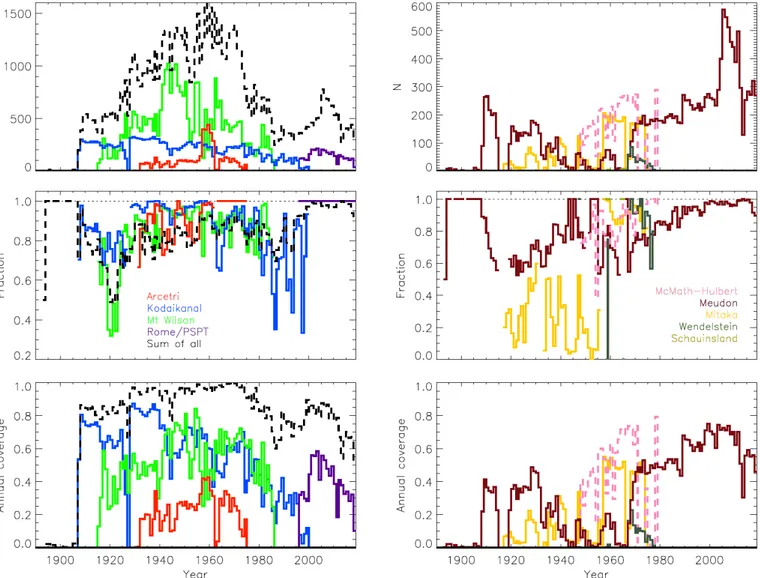
Figure 2 shows the annual distribution of the number and the fraction of the images from all the archives we used for our analysis. The fraction of days per year covered by each archive is also shown in Fig. 2, while Table 2 lists the number of the common observing days for the various pairs of all the archives used here.
As can be seen in Fig. 2, Me is the longest series among the ones included in this study, with data extending from 1893 to 2018. Me includes observations over 14512 days out of which 10880 days are from the photographic data. How-ever, there are currently very few or no digitised data over the periods 1893–1906, 1914–1918, and 1940–1961. Ko is the second longest series, with data for 18963 days in total with about one observation per day. However the amount of Ko images per year decreases with time and especially after 1990 remains very low. MW is the third longest series studied here. It includes observations from 13491 days, and generally multiple images were taken for each day of ob-servation. We notice that the amount of MW data during 1940–1950 is roughly 2–3 times larger than during other
pe-riods. With 4901 days over a period of 32 years, MM is the shortest series employed here other than Sc, and WS which are incomplete. Ar and Mi have less observations per year than the other archives, thus including 3573 and 3987 days of observation, respectively. Ar data exhibit a peak of im-age availability between 1957 and 1962. Due to the limited amount of Sc and WS data and taking into account the sim-ilarity of these observations, which were part of the same observing program of the Kiepenheuer-Institut für Sonnen-physik, we merged these two archives and we report results from both of these datasets as a single series.
2.2. Synthetic data
We also employed the synthetic images created by Chatzis-tergos et al. (2018b). In particular, in this study we used the subsets 1, 6, and 8 from Chatzistergos et al. (2018b) in their unchanged form. The basis for the synthetic data were the Rome/PSPT images covering the period 2000– 2014. Briefly:
– For subset 1, we employed contrast images, imposed on them the centre-to-limb variation (CLV, hereafter) com-puted as the average over all the available Rome/PSPT images, and applied a linear characteristic curve (CC, hereafter). We did not introduce any other image prob-lems so to create images that describe the best quality historical data. Subset 1 consists of 500 observations equally spaced in time during the period 2000–2014. – Subset 6 was created by using 10 observations, on which
we applied the same CLV and CC as in subset 1. How-ever, prior to the application of the CC, we imposed 20
Chatzistergos et al.: Segmentation of Ca II K SHG
different inhomogeneity patterns on the images. Each of these patterns was derived to replicate some of the common problems in the historical data and was used with 10 severity levels. Thus subset 6 includes 2000 im-ages representing observations with quality varying from very good to very poor.
– Subset 8 includes 2000 images, each one created with a random set of problems and severity level. In this sam-ple, the CC is in the form of a 3rd degree polynomial with random parameters for each image. The CLV pat-tern, the inhomogeneities with the corresponding sever-ity levels, and the vignetting were chosen randomly to replicate the most common features of the historical se-ries.
2.3. Time-series of plage areas
We will also compare our results with other existing plage area time-series. We considered the series of plage areas de-rived by Kuriyan et al. (1982), Foukal (1996)3, Ermolli et al.
(2009a), Ermolli et al. (2009b), Tlatov et al. (2009), Bertello et al. (2010), Chatterjee et al. (2016), Priyal et al. (2017), Singh et al. (2018), and those presented in the National oceanic and atmospheric administration Solar Geophysical data reports3(SGD, hereafter).
In brief, SGD provided monthly tables4 for the
plage areas derived from the MM (06/1942–09/1979), MW (10/1979–09/1981), and Big Bear solar observatory (10/1981–11/1987). The plage areas from the MM and MW archives were obtained from the physical photographs and drawings. According to Foukal (1993), this was done man-ually with prints of overlay surfaces, which included circles of different sizes and different positions on the disc in or-der to take the foreshortening into account. Sunspots were included in the plage areas. The processing of the Big Bear solar observatory data is described in Marquette (1992). Similarly, Kuriyan et al. (1982) derived plage areas from the physical Kodaikanal photographs. Foukal (1996) used uncalibrated MW data from the 8-bit digitisation and pro-duced the time-series (termed Apindex) by manually
select-ing the plage regions in every image. Ermolli et al. (2009a) used the available wedge exposures on the Ar plates to con-struct the CC and to calibrate the Ar images. Ermolli et al. (2009b) calibrated the Ar, Ko (8-bit), and MW (16-bit) data with a linear relation, derived for each image sepa-rately, and segmented the images with constant thresholds for the contrast and feature size. Tlatov et al. (2009) pro-cessed the data from Ko (8-bit), MW (16-bit), and Sacra-mento Peak observatories. The data were linearly scaled so that their CLV matched a reference one (see Chatzistergos 2017; Chatzistergos et al. 2018b) and then segmented with a threshold of a constant multiplicative factor to the full width at half-maximum of the distribution of intensity val-ues of the image (including the CLV). Bertello et al. (2010) processed uncalibrated MW 16-bit data. They calculated the histogram of contrast image values and defined a pa-rameter related to plage areas. This index does not carry 3 Available at https://www.ngdc.noaa.gov/stp/solar/
calciumplages.html
4
The report books are available at https://www.ngdc.noaa. gov/stp/solar/sgd.html. More information on the derivation of the plage areas is given in report No. 515-supplement from July 1987.
information on the absolute plage area, and needs to be cal-ibrated to a reference plage area series independently; see Sect. 5.2 for more details. Chatterjee et al. (2016) used un-calibrated 16-bit Ko data and identified the plage regions as those with C > Cmedian+ σ, where C is the contrast
of each pixel, Cmedian the median contrast of the disc and
σ the standard deviation of contrasts. Priyal et al. (2017) calibrated the 16-bit Ko data by applying an average rela-tion derived from the data that include a calibrarela-tion wedge and then segmented the data with constant thresholds to derive a plage area series. Singh et al. (2018) analysed the 16-bit Ko data. They manually selected the observations that were used for their plage areas time-series with the purpose of excluding data that have potentially been taken with different bandwidths or were centred outside the line core. It is worth noting that no data after 1976 were used in the time series of Singh et al. (2018).
We also considered one plage area record derived from Ca II K filtergrams taken at the San Fernando observatory (SFO) with the CFDT1 and CFDT2 (Cartesian full-disc telescopes 1 and 2, respectively). CFDT1 has been operat-ing since mid-1986, producoperat-ing images of 512 x 512 pixels with a pixel size of 5.1200/pixel. CFDT2 started operation in mid-1992 producing images of 1024 x 1024 pixels at a pixel size of 2.500/pixel. Both telescopes use filters centred on the Ca II K line with bandwidth of 9 Å (Chapman et al. 1997), i.e. considerably broader than the historical observa-tions and hence with stronger photospheric contribuobserva-tions.
It is worth noting that the above series were derived with rather different processing techniques and from different data, also obtained from diverse digitisations of the same archive, or from various samples of observations therein. Furthermore, none of the above studies attempted to com-bine plage series from different image sources.
3. Image processing
All together, we have analysed 99584 images from 8 differ-ent historical archives, of which only 82680 were used for our analysis. We also used 3292 (all available) images from the modern dataset of Rome/PSPT. We ignored all patho-logical cases . Specifically, we used 4825 Ar, 19291 Ko, 4911 MM, 17605 Me, 4193 Mi, 31430 MW, 3292 Rome/PSPT, 18 Sc, and 407 WS images. This required development of automated and robust correction and calibration methods the main steps of which are outlined in the following. Ap-pendices A and B describe in more detail how we sorted and pre-processed the data, as well the characteristics of the individual archives.
3.1. Photographic calibration and CLV compensation
After the pre-processing, the images analysed in our study were photometrically calibrated and compensated for the CLV as described by Chatzistergos et al. (2018b). Briefly, it is an iterative process to identify the quiet Sun (QS, here-after) background by applying a running window median filter after the active regions have been singled out from the solar disc. Assuming that the QS does not significantly vary with time (as suggested by several studies in the lit-erature, see Chatzistergos et al. 2018b, for more details), we relate the derived density QS CLV to the logarithm of intensity QS CLV we get from modern CCD-based
obser-A&A proofs: manuscript no. paper_segmentation_shg_18_arxiv
Fig. 2. The number of images per year from the different archives (see legend) considered in this study (top row), the fraction of the available images from each archive per year that we used for our final analysis (middle row), and the fraction of days per year covered by each archive (bottom row). For the sake of clarity, the analysed series were divided in two groups, shown in the left and right columns. Also shown is the sum from all archives (black line in the left panels).
Table 2. Number of common days for various pairs of the 9 Ca II K archives analysed in this study.
Ar Ko Me MM MW Mi Rome/PSPT Sc/WS Ar 3573 2218 617 1308 2194 839 0 109 Ko 2218 18963 4687 2820 8025 2418 33 242 Me 617 4687 14512 748 3284 781 2253 159 MM 1308 2820 748 4901 2915 1268 0 172 MW 2194 8025 3284 2915 13491 2083 0 256 Mi 839 2418 781 1268 2083 3987 0 127 Rome/PSPT 0 33 2253 0 0 0 3287 0 Sc/WS 109 242 159 172 256 127 0 411
vations. We thus derive a linear CC between the density and logarithm of intensity, which is used to calibrate the image and the QS CLV. We then produce contrast images as Ci = (Ii− IiQS)/I
QS
i , where Ci, Ii is the contrast and
the intensity of the ith pixel, respectively, while IiQSis the level of the QS intensity in the ith pixel. For our analy-sis, we only considered pixels within 0.99R to avoid the influence of the uncertainties in the radius estimates. This corresponds to µ = cos θ = 0.14, where θ is the
heliocen-tric angle. The accuracy in determining the edge of the disc is considerably higher for the Rome/PSPT images, so for these images we considered pixels within 0.9999R. Figure 3 shows the resulting calibrated and CLV-compensated im-ages for the observations displayed in Fig. 1. The Me and Rome/PSPT CCD data calibrated for instrumental effects were processed to compensate for the CLV in the same way as the historical data.
Chatzistergos et al.: Segmentation of Ca II K SHG
Fig. 3. Calibrated and CLV-compensated images derived from the observations shown in Fig. 1. The images have been corrected for artefacts as described in Sect. B and are compensated for ephemeris. All images are saturated in the range [-0.5,0.5].
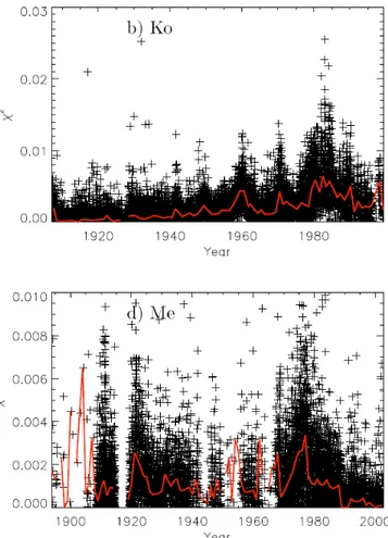
We consistently applied the image processing described above to data from different archives. In Fig. 4 we show the temporal variation of the reduced χ2 of the fits to derive
the CC for the data from Ar, Ko, MM, Me, Mi, and MW observatories. The goodness of the fit in this step mainly depends on three factors: the presence of strong artefacts over the recorded image of the solar disc, exposure prob-lems, and the similarity of the QS CLV measured on the historical data to the one we use as a reference. The lat-ter is essentially giving us an indication for changes in the bandwidth or the central wavelength of the observation. Hence abrupt and systematic changes in the determined χ2
of the fits are indications for changes in the instruments or in the observing conditions. It should be noted, however, that this is not a very strict criterion to identify all possible quality transitions in the archives, since multiple effects can counterbalance each other (e.g. use of narrower bandwidth when the observations suffer from vignetting effects). Figure 4 shows that the values of the plotted quantity do not sig-nificantly vary with time for Ar and MM, while they grad-ually increase with time for Ko. Besides, we notice a slight increase in the Ar values at approximately 1953, coincid-ing with the change in the spectrograph (see Appendix A). Furthermore, the values for MW show an abrupt jump be-fore 08/1923. This is attributed to an instrumental change reported in the MW logbooks as the implementation of a different grating since 21/08/1923. For the values of Mi we
see a jump after 02/1966 which coincides with instrumen-tal adjustments. We do not discern any difference in the χ2 of the fit around 1925, when the Mi observatory was
re-located, however the data points are too few to derive any meaningful conclusions about this. There are many changes in the χ2 of the fit for Me data, however we cannot derive any meaningful conclusions due to the low number of data for few years and the multiple digitisations within a given year. An exception is for the data around 1980, when there is a notable jump in the χ2 values. This can potentially be
attributed to the digitisations, since the data in the period 1970–1980 belong to a different digitisation than the ones after 1980. Furthermore, considering only the period after 1980 when we have sufficient data which derive from the same digitisation, we note that there is a small decrease in the χ2 after 1990.
3.2. Plage identification
We performed the disc segmentation with a variant of the method presented in Nesme-Ribes et al. (1996, NR, here-after) as used e.g. by Ermolli et al. (2009b). This method as-sumes a Gaussian background brightness distribution, while magnetic features add a non-Gaussian contribution to the wings of the distribution: at the low and high contrast for dark spots and bright plage, respectively. We first compute the mean contrast, ¯C, and the standard deviation of the
A&A proofs: manuscript no. paper_segmentation_shg_18_arxiv
Fig. 4. Temporal variation of the reduced χ2 of the fit performed on the QS CLV to determine the CC during the photometric
calibration of the images. The values shown here are for all images from the Ar (a), Ko (b), MM (c), Me (d), Mi (e), and MW (f) archives. For Mi we show the values for the images of the earlier (blue) and the more recent (black) digitisations separately. The red solid (yellow for the earlier Mi digitisation) line shows annual median values.
contrast, σC, over the disc. We identify pixels that have
con-trasts within ¯C ± kσCfor an array of values of k (typically
in the range 0.1 to 3.0). For these locations we calculate the mean contrast and the standard deviation. The minimum of the calculated mean contrasts, ¯Cmin, best represents the
background QS regions. The idea is that network and plage skew the distribution and cause ¯C to be shifted to positive values, while the darker spots and pores cover a sufficiently small part of the solar surface as not to dominate over the effect of plage and network. The value of k that gives the lowest mean contrast is adopted as the best representation
of the QS contrast. Nesme-Ribes et al. (1996) found that the optimum threshold K is the contrast that corresponds to a slightly higher value of k than kC¯min. They considered
values of k between 0.3+kC¯minand 0.6+kC¯min. However NR
aimed at identifying the QS, while we aim at segmenting the image, i.e. identifying plage features. For this purpose we consider a multiplicative factor, mp, to the standard
deviation within the disc. The contrast threshold used to identify plage is then given by the following equation:
Chatzistergos et al.: Segmentation of Ca II K SHG
Fig. 5. Segmentation masks derived from the observations shown in Fig. 1. Disc features shown are plage (orange) and quiet Sun (blue). The disc fraction covered by plage is given on the upper left side of each mask.
with mp= 8.5. This value was chosen so that when applied
to the Rome/PSPT we replicate the SRPM (Solar Radia-tion Physical Modelling, Fontenla et al. 2009) plage values. We note that the exact value of the segmentation parame-ter is not of great significance for the work presented here, where the aim is to compare and combine results from the various archives that have been processed consistently. For the segmentation, we only considered pixels within 0.98R for all archives to avoid uncertainties in the processing of the last few analysed pixels near the limb.
Figure 5 displays examples of the derived masks of plage features for the images shown in Fig. 1. These masks are used to calculate the disc fraction covered by plage regions. The same parameters were used to segment all images. We also produced time-series of the plage areas in millionths of solar hemisphere corrected for projection effects. To do that we computed the sum of the 1/µ of the plage regions, to account for projection effects, and normalised it to the area of the hemisphere.
4. Analysis of the Ca II K series
4.1. Day-by-day comparisons between datasets
There is, unfortunately, no single day, on which observa-tions from all historical archives considered in this study would be available. We have identified 91 days, on which
data from all historical archives other than Me, Sc, and WS are available. There is only one day of direct overlap of all archives, except Me, to either Sc or WS. Out of the 91 days on which most archives overlap we selected five days each within two days from an observations of Sc or WS to show in Fig. 1. In this figure one can easily spot the differences be-tween the archives, as well as within the same archive. The stray light conditions vary, with e.g. MM1 suffering worse conditions than Ar1. Ko and Mi observations were taken with a similar bandwidth, which is also the broadest among the historical data analysed here. We notice that the bright features in the Ko observations are slightly smaller com-pared to those in the other archives. Also sunspots are seen, while Me, MW, MM, and Ar images display filaments which are usually not found in the data from the other archives. The network cells and plage regions are more expanded in Ko2 compared to the other Ko observations shown in Fig. 1. The network cells are better seen and more expanded in Mi3 than in Ko3 even though the observations are sup-posed to be taken with the same bandwidth. MM seems to be more consistent than the other archives, although it suffers more strongly from exposure problems.
In Fig. 3 we notice that the contrast values of Ko images are lower than in the observations from the other archives taken with narrower bandwidth. Therefore, we expect the plage areas derived from these data to be lower than for the other archives. This is not the case for observation Ko2,
A&A proofs: manuscript no. paper_segmentation_shg_18_arxiv
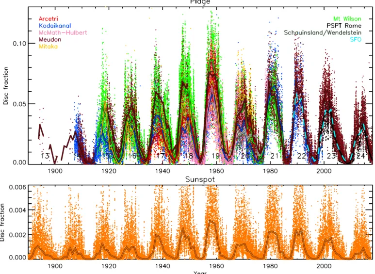
Fig. 6. Top panel: Fractional disc coverage by plage as a function of time, derived with the NR thresholding scheme applied with the same parameters on images from the Ar (red); Ko (blue); MM (pink); Me (brown); Mi (orange); MW (green); Sc/WS (dark green); Rome/PSPT (black) archives. Also shown are the plage areas from SFO (light blue). The numbers under the curves denote the conventional SC numbering. Bottom panel: Sunspot areas from Balmaceda et al. (2009). Individual small dots represent daily values, while the thick lines indicate annual median values.
which might be taken with a narrower bandwidth. We note, however, that the lower contrast can also be due to other reasons, such as stray-light, or even errors in the determi-nation of the CC during the calibration.
The segmentation masks for the different archives shown in Fig. 5 are rather similar, however some differences are noticeable. The individual regions identified as plage for the Ar, Ko Sc, and WS archives are smaller than those from MM, Me, Mi, and MW, in agreement with the dif-ferent bandwidth of the observations and the expansion of the features with height. However, this does not apply to the Mi data, which were nominally taken with the same bandwidth as Ko observations, but suffer from clear instru-mental and methodological issues. We also notice that more smaller regions are identified as plage for Mi and MW im-ages compared to those from the other archives, as well as that the boundaries of the identified features are smoother for MM and MW than for other data sources. This is most likely due to different seeing conditions at the locations of the observatories or possibly due to the digitisation as well.
4.2. Plage areas
Figure 6 shows the daily and the annual median values of plage areas in disc fractions for all the processed SHG data along with the Rome/PSPT data and the SFO series. The sunspot areas compiled by Balmaceda et al. (2009) are plotted in the lower panel for comparison. Consider-able scatter is seen in the daily values for solar cycles (SC, hereafter) prior to SC 21. The lower scatter for SC after SC 21 is, however, also partly due to the fewer considered archives over that period. The largest dispersion (up to 0.15 in disc fraction) during the activity maximum is seen for SC 18, while plage areas during SC 19 have a smaller scatter than in SC 18. We notice the same behaviour in SC 18 and 19 also in the sunspot areas by Balmaceda et al. (2009). On the whole, the computed plage areas agree reasonably well among all datasets. There is a disagreement between the plage areas from the various datasets for cycles 17 and 20, while the plage areas from Me and MW before 1970’s are higher by up to 0.03 (SC 18) than values derived from all other datasets. Me and MW include observations taken
Chatzistergos et al.: Segmentation of Ca II K SHG
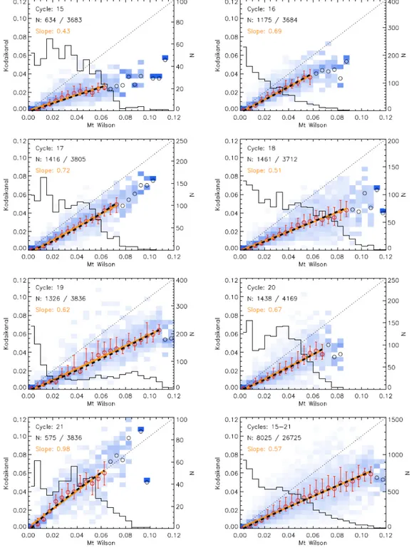
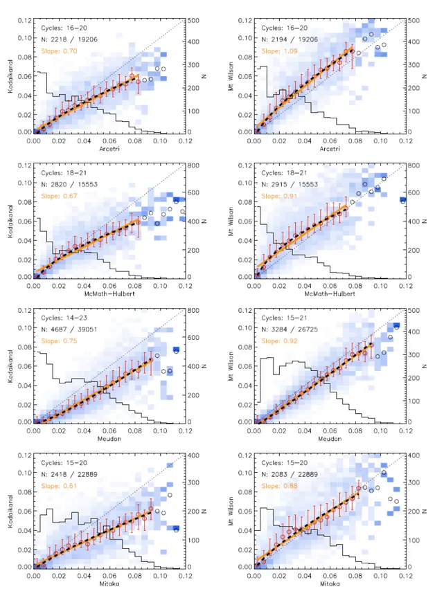
Fig. 7. Probability distribution functions (PDF) for fractional disc coverage by plage derived from Ko data, within area bins of 0.005, as a function of the disc fractions from MW for the same days. The PDF are colour-coded with white being 0 and bright blue 1. The Ko series is taken as the reference for this particular representation. Circles denote the average value within each column. For columns with less than 20 days of data these circles are shown in black, otherwise in red. We also show the asymmetric 1σ interval for each column. Two different fits to the average values are over-plotted; a linear fit (yellow) and a power law fit (black). The number of days included in each column is over-plotted with a solid black line (see right-hand axis). The dotted black line has a slope of unity and represents the expectation value. Each panel shows the PDF matrix for a given SC, while the lower right panel is for the whole interval of overlap between the compared series. The number of overlapping days used to construct each matrix (N) and the total number of days within each time interval is written in the plots. The slope of the linear fit is also given.
with a narrower bandwidth than most archives analysed here (only MM has a yet narrower bandwidth). This might explain the generally higher plage areas derived for those archives. The plage areas from Me match very well those from Ko for the period 1907–1914 hinting at a change in
the Me data around 1914 (see Fig. A.3 Me1). MW, with a broader nominal bandwidth than Me, gives higher plage areas over SC 19 than Me. This can be due to the reported narrower slit width used in MW as compared to the other observatories (see Pevtsov et al. 2016, for more details).
A&A proofs: manuscript no. paper_segmentation_shg_18_arxiv
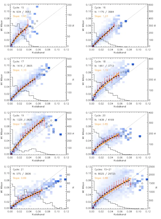
Fig. 8. Same as Fig. 7 but using MW plage area series as the reference and Ko as the secondary set.
Around 1980, the derived disc fractions from MW become lower than those from Ko, while the areas from Me are at a similar level to those from Ko. The Ko results would render SC 21 stronger than SC 19, which is in contrast to all other available data, and the sunspot areas. However, the results derived from the Ko series for SC 21 and 22 are less reli-able than those for earlier periods. This is due to the small number of observations over that period, the lower quality of observations than for other periods, the increase of the disc eccentricities with time (Ermolli et al. 2009b), and the
lower accuracy of the image processing for the data after 1980 attested by the clear trend in Fig. 7b). Nevertheless, studies in the literature also reported stronger amplitude for some solar quantities over SC 21 than SC 19. For instance, from their analysis of Kodaikanal white light data, Mandal & Banerjee (2016) found that SC 21 is stronger than SC 19 when considering sunspots with area lower than 0.001 in hemispheric fraction. Our results for MM, which has a similar bandwidth as Me, are closer to those from Ko than Me. However, the spatial resolution of MM data is lower
Chatzistergos et al.: Segmentation of Ca II K SHG
Fig. 9. Same as Fig. 7 but with Ko (left) and MW (right) plage area series as reference and Ar (1st row), MM (2nd row), Me (3rd row), and Mi (4th row) series as the secondary, by considering the whole period of observations over which the respective datasets overlap (see Table 2).
compared to the other datasets. Furthermore, the MM im-ages seem to suffer from poor seeing and stray-light more than other archives, which might also affect our results. The plage series from Mi data is not as reliable as the oth-ers due to the fact that the branch before 1957 consists of a rather small number of observations per year, commonly covering only January of each year. The lower values of Ar
before SC 19 can at least partly be explained due to the change in the spectrograph on 25/05/1953 (see Appendix A). The Rome/PSPT areas are systematically lower than those from Me, which is consistent with the difference in the bandwidths of their observations.
In Fig. 6, we also over-plotted the SFO values to bridge the Rome/PSPT and Ko series. These records appear to
A&A proofs: manuscript no. paper_segmentation_shg_18_arxiv
Fig. 10. Same as Fig. 7 but with Me plage area series as reference and Ar, Ko, MM, Mi, MW, and Rome/PSPT series as the secondary, by considering the whole period of observations over which the respective datasets overlap (see Table 2).
be consistent. The SFO plage areas match those from Rome/PSPT almost perfectly, while they are slightly higher than those from Ko during the maximum of SC 22. Con-sidering, however, that the plage areas from Ko during SC 21 and 22 are at a similar level to SC 19, this might hint to a possible underestimation of the plage areas in the Ko series before SC 21.
4.3. Comparison of plage series from individual archives Figures 7–10 show the relation between the derived plage areas from the various datasets. Following Chatzistergos et al. (2017) we chose one record to act as the reference and the other as the secondary one. We binned the disc fractional plage areas into bins of 0.005. The results do not change significantly with small variations of this value. We tested different bin sizes in the range 0.001–0.01 and found 0.01 to be too high to accurately sketch the relation very roughly, while 0.001 was too low and the bins did not in-clude a sufficient number of data points. We produce a list of all dates when the secondary has areas within a given bin.
For each such array of dates, we compute the histogram of the plage areas derived from the reference set. This results in a 2D matrix, every element of which contains the number of days for a given combination of plage areas measured by the two archives. Dividing each column by the total num-ber of occurrences for that column results in a probability distribution function (PDF). Figures 7–10 show the PDF of the plage areas of the reference archive for each bin value of the secondary one. In these plots we also show the average values of each PDF as red circles along with the asymmetric 1σ intervals. We applied two different types of fits to the av-erage values (also shown in the plots), namely a linear and a power law with an offset. We show results for individual SC, as well as for the whole period of overlap between the compared series.
Figure 7 displays the relation between Ko and MW with Ko acting as the reference record. The plage areas from MW data are consistently higher than the areas from Ko data with an almost linear dependence. The results also differ slightly from cycle to cycle, although SC 18 and 21 stand out. The PDF is significantly broader in SC 18, while for SC 21 the results from the two records are in almost
Chatzistergos et al.: Segmentation of Ca II K SHG
Fig. 11. Comparison of the plage areas derived here (black) to other published series based on the same datasets: (a)) Ermolli et al. (2009a, yellow) and Ermolli et al. (2009b, red) for Ar data; (b)) Chatterjee et al. (2016, blue), Priyal et al. (2017, red), and Singh et al. (2018, green) for Ko areas in disc fractions; (c)) Ermolli et al. (2009b, red), Kuriyan et al. (1982, yellow), and Tlatov et al. (2009, blue) for Ko areas in fractions of a hemisphere; (d)) Bertello et al. (2010, yellow), Ermolli et al. (2009b, red), Foukal (1996, green), Tlatov et al. (2009, blue), and SGD (pink) for MW data; (e)) SGD (pink) for MM data. The curves are annual median values. All panels except b) are in fractions of hemisphere corrected for projection effects. The numbers under the curves denote the conventional SC numbering.
perfect agreement with each other. Results for SC 19 show a greater number of days with large plage areas compared to other cycles. The distribution of MW plage areas over SC 19 shows a peak for plage areas less than 0.005 then decreases for areas 0.02–0.06 and exhibits another peak at
0.08–0.09. We notice that the linear fit performs almost as well as the power law function function for most SC. Overall a linear relation to calibrate the results from MW to Ko series seems to be a good choice for all the cycles. By using different methods, Tlatov et al. (2009) also compared
A&A proofs: manuscript no. paper_segmentation_shg_18_arxiv
Fig. 12. Scatter plots between the plage area values derived by other authors (y-axis) and those obtained here (x-axis): (a)) Ermolli et al. (2009a) for Ar data; (b) Ermolli et al. (2009b) for Ar data; (c)) Chatterjee et al. (2016) for Ko data; (d)) Ermolli et al. (2009b) for Ko data; (e)) Priyal et al. (2017) for Ko data; (f)) Tlatov et al. (2009) for Ko data; (g)) SGD for MM data; (h)) Bertello et al. (2010) for MW data; (i)) Ermolli et al. (2009b) for MW data; (j)) Foukal (1996) for MW data; (k)) Tlatov et al. (2009) for MW data; (l)) SGD for MW data. Blue asterisks (orange dots) show the annual (daily) values. In panel i) the green circles show the daily values excluding those from SC 19. The solid black lines have a slope of unity. The dashed (dotted) red lines are linear fits to the annual (daily) data. Also shown are the corresponding parameters of the linear fits to the annual values and the linear correlation coefficients of the annual values.
their plage areas from the Ko and MW series, by reporting a better agreement between the two series over SC 21 and a change in the relation over SC 19. However, in their results, the Ko and MW series agree also for SC 15–17.
Figure 8 displays the relation between Ko and MW results, now with the MW series acting as the reference
record. Most aspects seen in Fig. 7 are apparent here too, e.g. the peculiar relations for SC 18, 19, and 21, or the dis-tribution of plage areas over SC 19. However, the relation between the compared series now shows an obvious non-linearity, with the power law function being more
appro-Chatzistergos et al.: Segmentation of Ca II K SHG
Fig. 13. Same as Fig. 12 but now comparing the plage areas derived by SFO (y-axis) and those obtained here (x-axis): (a)) for Ko data; (b)) for Me data; (c)) for Rome/PSPT data.
priate to describe the relation between Ko and MW plage areas.
We obtain similar results when comparing the plage area series from the other archives, however with poorer statistics since the overlap between the compared archives is shorter. Figure 9 shows the same matrices as in Fig. 7 and 8, now for the Ar, MM, Me, and Mi archives and using Ko and MW as the references, due to their better tempo-ral coverage. We notice a slight discontinuity in the disc fraction values from the Mi data compared to those from MW around 0.04, before which the areas from MW are higher than those from Mi but become lower after it. This discontinuity is also seen when compared to Ko plage ar-eas. We investigated the reasons for this discontinuity and found that it can be attributed most likely to the instru-mental changes that occurred around 1966, however we can-not exclude as probable reason the change of photographic medium on 02/03/1960.
It is worth noting that most of the relations shown in Fig. 9 are to a good extent linear. The Ar and MM data seem better fitted with the power law function for both Ko and MW as the reference, however the difference to the linear relation is minute.
In a similar manner as Fig. 7–9, Fig. 10 compares the Me data to the other archives, now using Me as the reference. Note that the overlap of the Me data with the Ar, MM and Mi series is limited to roughly 700 days each, and in par-ticular the low-activity periods are poorly represented. The overlap is somewhat better with Ko, MW and Rome/PSPT. The relationship with MW is, to a good degree, linear, while the relationship to Ko and Rome/PSPT is non-linear. The spread of the PDF for the comparison of Me to Rome/PSPT is lower than for the other archives. We note here that for the comparison to Rome/PSPT shown in Fig. 10 we used the Me data taken with a CCD and those stored in photo-graphic plates. We also compared the Rome/PSPT series to the CCD and photographic plate Me data separately (shown in Fig. D.1) and the results are almost the same in all cases.
Unfortunately, no historical archive, other than Me, has a statistically significant overlap with the Rome/PSPT dataset therefore we cannot perform any meaningful com-parison of results from modern and the other historical ob-servations.
4.4. Comparison to other plage area records
In Fig. 11 we compare annual means of our plage areas from individual archives with those available in the literature. Panels a) to e) show results derived from the Ar, Ko, MW, and MM observatories. To our knowledge, there are no pub-lished results for the Me, Mi, Sc, or WS data to compare to. The various series are all given in hemispheric fractions except the Ko series by Chatterjee et al. (2016), Priyal et al. (2017), and Singh et al. (2018), which are in disc fractions. To compare our results directly with the published series we show values of hemispheric fraction for all archives, but for Ko we also show values in disc fractions (panel b)). The series by SGD, Foukal (1996), Ermolli et al. (2009a), Er-molli et al. (2009b), Chatterjee et al. (2016), Priyal et al. (2017), and Singh et al. (2018) have daily cadence. We com-puted annual median values in the same way as we did for our results. The Ko series by Tlatov et al. (2009) is given in monthly means, while all other series are provided as annual mean values.
Ar images were previously analysed by Ermolli et al. (2009a) and Ermolli et al. (2009b). Figure 11 a) shows that our series and that by Ermolli et al. (2009b) agree well, while the one by Ermolli et al. (2009a) is consistently lower. Our areas are at a similar level as those by Ermolli et al. (2009b) after 1955, but higher before that. As can be seen in Fig. 7 of Ermolli et al. (2009b), their plage ar-eas from Ar images during SC 17 are too low compared to those obtained from MW and Ko images. This supports the area values obtained here. However, the amount of im-ages used in our study before 1950 is lower than that in Ermolli et al. (2009b), which could also contribute to the above mentioned discrepancies.
The Ko images were analysed by Kuriyan et al. (1982), Ermolli et al. (2009b), Tlatov et al. (2009), Chatterjee et al. (2016), Priyal et al. (2017), and Singh et al. (2018). Our ar-eas as well as those by Tlatov et al. (2009), and by Ermolli et al. (2009b) were derived from images from the earlier 8-bit digitisation of the Ko images, while the results by Priyal et al. (2017), Chatterjee et al. (2016), and Singh et al. (2018) are from the latest 16-bit digitisation. The results by Kuriyan et al. (1982) are from the physical pho-tographs. Our Ko plage areas series is close to the one re-ported by Ermolli et al. (2009b, Fig. 11 c)), although it is higher for SC 21 and 22. The agreement to the series by Singh et al. (2018) is also good, except for SC 14, when the
A&A proofs: manuscript no. paper_segmentation_shg_18_arxiv
areas by Singh et al. (2018) are twice as high as ours. The series by Chatterjee et al. (2016) and Tlatov et al. (2009) are systematically higher, while the one by Priyal et al. (2017) is almost consistently lower than ours for most SC except for SC 17, 19, and 20 (Fig. 11 b)). The values in the series by Kuriyan et al. (1982) are consistently lower than ours except for SC 14. The plage areas by Chatterjee et al. (2016) show SC 18, 19, 21, and 22 at roughly the same levels. We can identify three potential reasons that cause the plage areas in the Chatterjee et al. (2016) to be higher than the other series: 1) In the study by Chatterjee et al. (2016) active regions were not excluded when calculating the standard deviation over the disc, which is then used as the threshold to segment the images; 2) bright regions were included when computing the map used to correct for the limb darkening, which reduces the contrast of plage re-gions (cf. Chatzistergos et al. 2018b) and hence renders the plage regions closer to the contrast range of the QS; and 3) a threshold equal to the value of the standard deviation of the disc was used for the segmentation. We applied the same segmentation method as Chatterjee et al. (2016) on Rome/PSPT data and found that a multiplicative factor of 1.45 to the standard deviation is needed to best match the disc fraction derived with our method. The first two issues have unpredictable effects on the derived disc frac-tions, while the third one merely suggests that the method applied by Chatterjee et al. (2016) includes fainter regions than with our method.
Figure 11 d) shows that our results from the MW series are in good agreement with those by Bertello et al. (2010) and Tlatov et al. (2009). We note, however, that we rescaled the series by Bertello et al. (2010) to match ours by applying a linear relation. Our plage areas and those from Bertello et al. (2010) are systematically higher than or equal to those derived by Ermolli et al. (2009b) and Foukal (1996), except for SC 19. The areas by Foukal (1996) are slightly lower than those by Ermolli et al. (2009b), except for SC 19 for which Foukal (1996) finds considerably higher areas. The areas for MW included in the SGD series for SC 21 are lower than all other series. Overall, the results from the various studies for the MW plage areas show a better agreement than those from Ko.
Finally, Fig. 11 e) displays that our MM plage areas agree rather well with those by SGD. Our results disagree in 1979, but our value for that year stems from merely 6 images and hence is not representative. The series by SGD is higher than ours before 1950. This is in agreement with the comment by Foukal (1996) that the plage areas by SGD for these years are inflated.
We note that Priyal et al. (2017) compared their Ko plage areas to those by Foukal (1996) for MW data and found a good match between the two series, except for SC 18 and 19, for which the areas by Priyal et al. (2017) were lower by 20%. Chatterjee et al. (2016) compared their Ko plage areas to MW areas by Bertello et al. (2010) and found a very good match, except during SC 19 and 22, for which the areas by Chatterjee et al. (2016) were lower and higher, respectively.
It is worth noting that the annual values shown in Fig. 11 include all observations analysed by each study, and the data included during a given year may vary among the series. This might also contribute to differences between the various time-series obtained here and in earlier studies. However, the main differences come likely from the
cali-bration, CLV compensation, and segmentation schemes ap-plied by the various studies. For instance, SGD, Kuriyan et al. (1982), and Foukal (1996) segmented the images by manually selecting the plage regions rather than using an objective criterion. Artefacts in the images which were in-troduced by the processing or were not adequately removed, affect the results of all series. Such artefacts can appear as dark regions, reducing the recovered area of plage, or bright regions which could be misidentified as plage. An-other critical issue is the definition of plage, which differs from study to study and is rather arbitrary. Therefore, cau-tion is needed even for the images for which different series give similar plage areas, since this can also be by chance.
Figure 12 shows scatter plots between our plage area series and those by Bertello et al. (2010), Chatterjee et al. (2016), Ermolli et al. (2009a), Ermolli et al. (2009b), Foukal (1996), Priyal et al. (2017), Tlatov et al. (2009), and SGD. For the series for which daily values are available we com-puted annual values for the common days only. This way we remove uncertainties due to potential differences in data selection. The relationship between our series and those by the aforementioned authors is almost linear once we restrict the comparison to data recorded on the same days. The agreement between our results and those by Ermolli et al. (2009b) for Ar, Ko, MW data and Bertello et al. (2010) and Tlatov et al. (2009) for MW data is good, with Per-son’s correlation coefficients of 0.96–0.99.
The scatter for Ko data from Chatterjee et al. (2016) and Priyal et al. (2017), MW data from Foukal (1996), and SGD for MM and MW data is too high to derive any mean-ingful conclusions. There are hints for non-linearity for the comparison to Chatterjee et al. (2016); Priyal et al. (2017), and Tlatov et al. (2009) for Ko data and Foukal (1996) for MW data at high plage areas. However, for Foukal (1996) this is almost entirely because of results over SC 19, when Foukal (1996) reports significantly higher plage areas than all other available results (Fig. 11 d)). In Fig. 12 j), all daily values are shown in orange, and those excluding SC 19 are in green. The saturation is no longer evident, while the scat-ter is slightly reduced. We also notice that removing SC 19 slightly increases the Pearson’s correlation coefficient be-tween the two series for daily values to 0.87 instead of 0.85. This was also reported by Ermolli et al. (2009b) when com-paring their results for the plage areas from MW and those by Foukal (1996).
Figure 13 shows scatter plots between the plage ar-eas from SFO and those derived here for Ko, Me, and Rome/PSPT. All three series show a linear relation with Person’s correlation coefficients of 0.97, 0.98, and 0.99 for the Ko, Me, and Rome/PSPT series, respectively. The slopes of the linear fit are 1.05, 0.79, and 0.99 for Ko, Me, and Rome/PSPT respectively. The slopes for the fit of the Me and Rome/PSPT to the SFO series is consis-tent with the difference in the bandwidths of the archives. Rome/PSPT used a broader bandwidth than Me, thus re-sembling more the SFO series. The fit of the Ko series to SFO gives a slope greater than that of the Rome/PSPT which is contrary to expectations due to Ko having em-ployed a bandwidth between those of Me and Rome/PSPT. This again hints for a problem with the Ko series over SC 22 (see also Sec. 4.2).
Chatzistergos et al.: Segmentation of Ca II K SHG
5. Effect of image processing on derived disc
fractions
A number of plage area series have been presented in the literature. They have been derived from SHG archives us-ing different methods. In particular, Foukal (1996, 1998); Foukal & Milano (2001); Bertello et al. (2010), and Chat-terjee et al. (2016) analysed uncalibrated SHG, while Priyal et al. (2014, 2017) and Tlatov et al. (2009) used basic cal-ibration techniques. Also, various authors used different methods to process the data and correct for artefacts in the historical images (Caccin et al. 1998; Worden et al. 1998; Zharkova et al. 2003; Lefebvre et al. 2005; Ermolli et al. 2009b,a), while others did not do such corrections, to our knowledge (Ribes & Mein 1985; Kariyappa & Pap 1996). Therefore, here we address the question, how the various image processing approaches affect the derived plage areas. For this, we use part of the synthetic data created by Chatzistergos et al. (2018b), which were introduced in Sec-tion 2.2. In the following, we compare the plage disc frac-tions derived in the original Rome/PSPT observafrac-tions to those from the synthetic images processed with our method and other methods presented in the literature. The results of this comparison for the synthetic data are summarised in Table 3.
5.1. Photometric calibration and CLV compensation
We first compared the results from uncalibrated data to those derived from images calibrated with our method. The uncalibrated data were processed with different methods to compensate for the CLV, namely the methods by Chatzis-tergos et al. (2018b, our method), Worden et al. (1998), Priyal et al. (2014), and by using the imposed background to remove the CLV. Recall that the CC is a logarithmic function and has to be applied on the images that include the CLV in order to mimic the historical data. Using the im-posed background is therefore an idealised situation where there are no errors in the image background calculation and all artefacts are removed completely. For subset 8 we also tested the calibration method by Priyal et al. (2014). Priyal et al. (2014) applied the average CC to all images derived from the calibration wedges. Thus, we computed the CC averaged over all imposed CC, which had been ran-domly generated to create subset 8, and applied it on all the data. When using the calibration of Priyal et al. (2014) we considered two separate cases for the CLV compensa-tion, using the imposed background and the method by Priyal et al. (2014). We did not test the calibration or CLV-compensation method by Tlatov et al. (2009), because we could not replicate it with the available information. For all these cases we performed the same segmentation with the NR method, which was applied to obtain the results pre-sented in Section 4, while using also the same segmentation parameters employed for all the analysed data.
The values in Table 3 show that the plage areas derived from the synthetic data with our processing are closest to the original ones for subsets 1 and 8, with differences being less than 0.003 and 0.025, respectively. For subset 6, the discrepancies remain quite low too, below 0.029. It is worth noting that a linear relation was initially imposed only on the data of subsets 1 and 6, while random non-linear rela-tions were imposed on the data of subset 8.
The accuracy of the CLV-compensation plays an im-portant role in the determination of the plage areas. All methods except that by Worden et al. (1998) return com-parable results in the absence of strong artefacts over the disc (subset 1). However, in the presence of artefacts (sub-sets 6 and 8) we see increased errors in the plage areas with all of them. The methods by Worden et al. (1998) and Priyal et al. (2014) result in disc fractions with greater dif-ferences to the original ones than with our method. The method of Worden et al. (1998) performs better than the one of Priyal et al. (2014) in subset 8. We also note that the linear correlation coefficient for the results with the method by Priyal et al. (2014) is rather low ( < 0.5) in all cases con-sidered here except for subset 1, which is representative of the best quality historical data unaffected by instrumental and operational issues.
The CC affects the dynamic range of the contrast im-ages in a non-linear way (remember that the CC is the relation between the logarithm of intensity and density). NR accounts for the change in dynamic range of the QS. However, errors are introduced to the plage areas due to the non-linearity affecting the plage regions. This can be seen in the case where we compensated the CLV with the imposed one. For this case there are no errors in the calcu-lation of the background but the differences to the original plage areas reach 0.044 in subset 8.
The top panel of Fig. 14 shows the difference between the plage areas of subset 8 derived with the different meth-ods and those from the original Rome/PSPT images. For all methods but ours the differences vary in-phase with the SC.
We repeated the above analysis by adjusting the seg-mentation parameters used in each method, except ours, so as to minimise the RMS difference in the disc fractions obtained from the various series to that from the original Rome/PSPT data. The results for subset 8 are shown in the bottom panel of Fig. 14. After adjusting the segmentation parameters we get comparable disc fractions with all meth-ods, with mean differences varying between 10−4 for our calibration and 10−3 for Worden et al. (1998). We notice that after adjusting the segmentation parameters the SC dependent variation is minimised from all series, however it is more evident in the results with the method of Worden et al. (1998). This confirms that the method of CLV removal by Worden et al. (1998) is affected by the activity level and returns erroneous results for the active region areas. The differences in the plage areas for subset 1 to the original Rome/PSPT data are qualitatively the same, though with lower values.
Overall, our results indicate that the photometric cali-bration of the images is not the most critical step for de-riving the plage areas. However, plage areas from the un-calibrated data can be significantly affected by the errors in the calculation of the CLV and subsequent feature seg-mentation. Our results also indicate that it is possible to get accurate plage areas from different historical archives without the need to adjust the processing method or rede-fine the segmentation parameters, provided the images are accurately calibrated and have been taken with the same bandwidth.