As far as the laws of mathematics refer to reality, they are not certain; and as far as they are certain, they do not refer to reality.
(Albert Einstein)
The Guide is definitive. Reality is frequently inaccurate. (Douglas Adams)
The work presented in this Ph.D. thesis deals with the definition of new fuzzy models for Group Decision Making (GDM) aimed at improving two phases of the decision process: preferences expression and aggregation. In particular a new preferences model named Fuzzy Ranking has been defined to help decision makers express fuzzy statements on available alternatives in a simple and meaningful form, focusing on two alternatives at a time but, at the same time, without losing the global picture. This allows to reduce inconsistencies with respect to other existing models.
Moreover a new preference aggregation model guided by social influence has been described. During a GDM process, in fact, decision makers interact and discuss each other exchanging opinions and information. Often, in these interactions, those with wider experience, knowledge and persuasive ability are capable of influencing the others fostering a change in their views. So, social influence plays a key role in the decision process but, differently from other aspects, very few attempts to formalize its contribution in preference aggregation and consensus reaching have been made till now.
In order to validate the defined models, they have been instantiated in two application contexts: e-Learning and Recommender Systems. In the first context, they have been applied to the peer assessment problem in massive online courses. In such courses, the huge number of participants prevents their thorough evaluation by the teachers. A feasible approach to tackle this issue is peer assessment, in which students also play the role of assessor for assignments submitted by others. But students are unreliable graders so peer assessment often provides inaccurate results. By leveraging on defined GDM models, a new peer assessment model aimed at improving the estimations of student grades has been proposed.
With respect to Recommender Systems, the group recommendation issue has been tackled. Instead of generating recommendations fitting individual users, Group Recommender Systems provide recommendations targeted to groups of users taking into account the preferences of any (or the majority of) group members together. The majority of existing approaches for group recommendations are based on the aggregation of either the preferences or the recommendations generated for individual group members. Customizing the defined GDM models, a new model for group recommendations has been proposed that also takes into account the personality of group members, their interpersonal trust and social influence.
The defined models have been experimented with synthetic data to show how they operate and demonstrate their properties. Once instantiated in the defined application contexts, they have been experimented with real data to measure their performance in comparison to other context-specific methods. The obtained results are encouraging and, in most cases, better than those achieved by competitor methods.
Introduction ... 9
PART 1: Fuzzy Models for Group Decision Making 1 Background on Group Decision Making ... 15
1.1 Decision Making ... 15
1.2 Group Decision Making ... 18
1.3 Preliminaries on Fuzzy Sets ... 21
1.4 Fuzzy Preferences Modeling in GDM ... 25
1.5 Fuzzy Preferences Aggregation in GDM ... 28
1.6 Fuzzy Alternatives Ranking in GDM ... 33
1.7 Dealing with Incomplete Information ... 35
2 Modeling Expert Preferences with Fuzzy Rankings ... 39
2.1 Ordinal Rankings ... 40
2.2 Evolution to Fuzzy Rankings ... 42
2.3 From Fuzzy Rankings to FPRs ... 44
2.4 From FPRs to Fuzzy Rankings ... 48
2.5 Partial and Multiple Fuzzy Rankings ... 50
2.6 Similarity Between Fuzzy Rankings ... 54
2.7 Comparison with Related Works ... 57
3 A Fuzzy GDM Model Guided by Social Influence ... 59
3.1 Theory of Social Influence and Opinion Change... 60
3.2 Outline of the Proposed Model ... 62
3.3 FPRs and SIN Generation ... 65
3.4 Using Social Influence to Estimate Missing Preferences ... 67
3.5 Preferences Evolution and Best Alternative Selection ... 69
3.6 Numerical Example ... 73
PART 2: Applications
4 Applications to e-Learning ... 89
4.1 Student Assessment in Massive Courses ... 89
4.2 Peer Assessment Methods ... 92
4.3 Formalization of the Peer Assessment Problem ... 96
4.4 Measuring Peer Assessment Performance... 99
4.5 Peer Assessment Methods based on Graph Mining ... 101
4.6 Fuzzy Ordinal Peer Assessment ... 105
5 Applications to Recommender Systems ... 113
5.1 Recommendation Algorithms ... 114
5.2 Measuring Recommendation Performances ... 118
5.3 Group Recommendation Strategies ... 122
5.4 A GDM Model for Group Recommendation ... 125
5.5 Influence-Based Recommendations ... 132
5.6 Comparison with Related Works ... 138
6 Experiments and Evaluation ... 143
6.1 GMPA with Synthetic Data ... 143
6.2 GMPA with Real Data ... 154
6.3 FOPA with Synthetic Data ... 158
6.4 FOPA with Real Data ... 168
6.5 FOPA vs. GMPA with Real Data ... 174
Final Remarks ... 183
Everyone’s life is full of alternatives. In fact, from the early days of life to a venerable age, from morning awakening to nightly sleeping, a person needs to make decisions of some sort. So, decision making can be considered one of the most important and frequent human activities. It includes information gathering as well as data mining, modelling, and analysis. It requires formal calculus and subjective attitudes and may take different forms according to situations and circumstances.
One of the most complex decision making structures arises when several persons are involved in the decision process. This is known as Group Decision Making (GDM). GDM has been widely studied since it has applications in many fields. Several models and tools have been proposed for supporting this process in each of its steps, from the expression of the decision makers’ opinions to their aggregation, from the selection of a feasible alternative to the achievement of the consensus on it. Among such approaches, those based on the Fuzzy Sets Theory, have shown to be the most effective to deal with the intrinsic uncertainty and imprecision of human judgments.
Nevertheless, fuzzy GDM models are not free of defects. In particular, the way decision makers express their preferences is often complex and requires to specify the degree to which each alternative is preferable to each other. This may result difficult and time-consuming and is likely to introduce errors and inconsistencies impacting the whole decision process. Moreover, even if several methods exist to integrate preferences expressed by decision makers, few attempts have been done till now to also consider social elements affecting the decision process like personality, interpersonal trust and influence.
To overcome these issues, in this Ph.D. thesis, new fuzzy models for GDM affecting both preferences expression and aggregation have been defined and
experimented within two application contexts: e-Learning and Recommender Systems. The thesis is organized in two parts: in part 1 (chapters 1-3), the proposed models are defined and experimented in-silico to demonstrate their properties; in part 2 (chapters 4-6), the defined models are instantiated in the selected contexts and experimented to measure their performance, also in comparison with other context-specific methods.
In particular, chapter 1 introduces the main concepts related to decision making, GDM and Fuzzy Sets, that are pre-requisite for the definition of the original models and methods described subsequently. The application of fuzzy sets to GDM is discussed and the most diffused fuzzy models and methods to represent and aggregate decision makers’ preferences, rank the problem alternatives and identify the best solution are introduced. Fuzzy-based methods for the management of incomplete information are also described.
In chapter 2, the original Fuzzy Ranking model for preference elicitation is defined and compared with related work. After having deepened the classical ordinal ranking model, the proposed model is described as a fuzzy extension of the ordinal one. Conversion algorithms from fuzzy rankings to fuzzy preference relations and backward are then defined as well as similarity measures evaluating the concordance between experts’ opinion.
In chapter 3 a Social Influence-Guided GDM model, able to manage the effects of social influence in GDM, is defined. The model estimates the level of social influence basing on interpersonal trust with the assumption that, the more a decision maker trusts another, the more her opinion is influenced by him. After having introduced background concepts on social influence and related theories, the proposed model is outlined and described in each step. The advantages with respect to other existing models are then presented as well as the results of an in silico experiment.
In chapter 4, the application of the defined models to peer assessment in standard and massive e-Learning contexts is discussed. The peer assessment problem is described and formalized, existing approaches, aimed at improving peer assessment reliability are outlined and performance measures capable of
establishing and comparing the goodness of different approaches are defined. Then, a new approach based on the instantiation on the defined GDM models is presented and compared with other existing methods.
In chapter 5, the application of the defined GDM models to the group recommendation problem (in the domain of Recommender Systems) is shown. After having introduced the most diffused approaches to individual and group recommendation, an original influence-based approach, based on the defined models, is defined and compared with related work. When generating group recommendations, the proposed model is able to take into account not only individual preferences (like most competitor methods) but also social elements like the personality of group members, their influence and mutual relationships.
In chapter 6, a set of experiments aimed at measuring the performance of the original peer assessment and group recommendation methods defined in chapters 4 and 5 are presented and compared with those obtained by other methods from the respective fields. Large-scale experiments with synthetic realistic data as well as small-scale experiments with real data have been performed. Results obtained, in both contexts, are encouraging and proposed methods, in most cases, outperform competitor methods.
PART 1
Fuzzy Models for Group Decision
Making
Background on Group Decision
Making
This chapter presents the basic concepts of Decision Making (DM) and Group Decision Making (GDM), which are the basis for the definition of the original models and methods described later on. Then, essential notions on Fuzzy Sets are outlined and their application in a GDM process, as a way to deal with the inherent uncertainty and imprecision of human judgments, is discussed. To this end, the most diffused fuzzy models and methods able to represent and aggregate decision makers’ preferences, to rank problem alternatives and to identify the best solution are described. Eventually, existing fuzzy-based methods that support incomplete and incoherent information processing in GDM are introduced.
1.1 Decision Making
Decision Making (DM) is a problem-solving activity aimed at the selection of a belief or a course of action among several alternatives. The typical DM process consists in the evaluation of the existing alternatives and the choice of the most satisfactory one, taking into account all the factors and contradictory requirements and according to the preferences of the decision-maker. It is therefore a process that can be more or less rational and based on explicit or implicit knowledge.
Any person makes decisions each and every day, often in an automatic and subconscious way. Some of these decisions are relatively small, such as deciding what to wear or what to have for lunch. Others are big and can
have a major influence on the course of our life, such as deciding where to go to school or whether to have children. Some decisions take time while others must be made in a split-second.
If we look at organizations, we see that any of them has its goals and achieves them through the use of resources such as people, material, money, and the performance of managerial functions such as planning, organizing, directing, and controlling. To carry out these functions, managers, at various levels, are engaged in a continuous DM process related to problems that can concern aspects of logistics management, customer relationship, marketing, production planning, etc. [1].
Making a correct decision is not always easy. In many cases, in fact, the identified alternatives are related to complex situations that may have several factors of uncertainty like [2]:
• impossibility or inexpediency of obtaining sufficient amounts of reliable information;
• lack of reliable predictions of the characteristics and behavior of complex systems that reflect their response to external and internal actions; • poorly defined goals and constraints in the project, planning, operation,
and control tasks;
• impossibility of formalizing a number of factors and criteria.
In [1], the authors recognize that the DM process within organizations is even more complex today than in the past. This is explained by several factors like the availability of huge amount of information that fosters the generation of more and more alternatives; the amplified cost of making errors thanks to the complexity of operations, automation, and the chain reaction that an error can cause in many parts of the organization; the rapid changes in the environment that introduce uncertainty and require decisions to be made quickly. These reasons justify the requirement for increasing technical and methodological support to help DM.
A typical DM process can be split in four phases as shown in Figure 1 [3]. In the intelligence phase the reality is examined, the problem is identified,
its limiting factors are analyzed and the problem statement is defined. In the design phase, a simplified model that represents the fragment of reality under examination is constructed and validated, and potential alternative solutions are identified. In the choice phase the identified alternatives are analyzed and a solution to the problem is proposed and tested to determine its viability. In the implementation phase the proposed solution is adopted. At every step it is possible to return to an earlier phase to refine the intermediate outcomes basing on their validation.
Figure 1. Steps of a DM Process
According to several authors [1, 2, 3] DM problems can be classified based on their structure. In structured problems, involved entities and relationships are convincingly established so that they can be numerically estimated. Such problems can be described and analyzed through standard mathematical models and methods coming from the fields of operational research, business analytics, simulation, statistics, forecasting, mathematical optimization, etc. Such problems are also referred to be “quantitatively formulated”.
Intelligent Phase Design Phase Choice Phase Implementation Phase Reality of Situation Problem Statement Alternatives Solution Model Validation Solution Testing Solution Adoption Assumptions
Conversely, in unstructured problems, only the description of the most important entities is available while quantitative relationships between them are not known. These problems are also known as “qualitatively expressed” and cannot be described and analyzed through standard models and methods. Typical unstructured organizational problems include planning new services, hiring an executive, initiate a research and development project, etc..
According to [2, 4], a feasible (and sometimes the only possible) way to address this class of problems is to rely on the formulation of subjective estimates carried out by decision-makers (thus based on their own ideas on the efficiency of possible alternatives and importance of diverse criteria) and on the definition of the corresponding preferences. The heterogeneous and qualitative parameters of the problem can be so combined into a unique model, which permits alternatives to be evaluated.
The assumption is that experienced managers perceive, in a broad and well-informed manner, how many personal and subjective considerations they have to bring into the DM process. On the other hand, successes and failures of the majority of decisions can be judged by people on the basis of their subjective preferences.
In the middle between structured and unstructured problems, there are semi-structured problems having both quantitative and qualitative elements. Solving them involves a combination of traditional analytical models with models based on subjective preferences. Unstructured and semi-structured DM problems are also called ill-structured.
1.2 Group Decision Making
Decisions can be made by individuals or groups. While individual decisions are often made at lower managerial levels and in small organizations, group decisions are usually made at high managerial levels and large organizations. The DM process in which there is more than one individual involved is named Group Decision Making (GDM).
GDM is particularly useful when decisions require multiple perspectives and different areas of expertise. The main advantages of GDM, if compared to standard GM, can be summarized as follows [5]:
• more intellectual resources are gathered to support the decision including individual competencies, intuition, and knowledge;
• the work related to acquiring and processing the amount of available information can be distributed among group members;
• if the group exhibits divergent interests, the final decision tends to be more representative of the needs of the organization.
GDM can be cooperative or non-cooperative. In cooperative GDM all the members, each with their own knowledge, ideas, experience and motivation, are supposed to work together to achieve a common decision for which they will share the responsibility. Conversely, in non-cooperative GDM (otherwise known as non-cooperative multi member DM), the group members play the role of antagonists over some interest for which they must negotiate.
As in cooperative GDM the members share responsibility for the decision (and may also participate in its implementation), it is important to assure that each member is satisfied with it. For this reason, the ideal condition to terminate a GDM process is the achievement of a unanimous solution. In absence of unanimity, the most satisfactory alternative for the group should be selected. The most common approaches to find it are [1]:
• the group decision is made by the group leader after having discussed with the other group members (authority rule);
• the group decision is made by selecting the alternative that is preferred by the majority of members (majority rule);
• the group decision is made by repeatedly eliminating the most unpopular alternative until just one is left (negative minority rule);
• the group decision is constructed by combining ranking or scores provided by members, individually, for each alternative (ranking rule);
• the group decision is constructed to minimize the group discordance so that no member is extremely dissatisfied (soft consensus rule) [6].
As a matter of fact, the commitment to the implementation of a given solution strictly depends upon the level of consensus achieved by the group. According to this principle, a decision imposed by a dominant portion of the group has to be considered worse than a decision obtained achieving genuine consensus. The most common reasons for discordance among the group members can be summarized as follows [2]:
• although the group members are supposed to share the primary goal (i.e. to find the solution which most benefits the organization), they can have hidden or just partially shared secondary goals (e.g. to meet the priorities and needs of their respective departments);
• each member may have a distinct perception of the problem and intuition which may be hard to formalize and share to the group;
• each member may have access to different profiles of information, certain members may also have privileged access to restricted information. These factors can be mitigated by promoting discussions and sharing all relevant information pertaining to the decision. However, even when this happens, there are other factors that can adversely affect the decision process like the need to obtain a solution rapidly or the pressure of concordant majorities on the other decision makers. Both factors are reflected in the group’s tendency to prematurely converge on sub-optimal solutions [7, 8].
Some authors [1, 2, 9] stress the importance of including a moderator to support the GDM process. The moderator defines the process rules, assigns the tasks of each member, selects the appropriate technology, develops the schedule to be accomplished, identifies controversial opinions, promotes the discussion on them and verifies the reached level of concordance [10]. As shown in [11], the participation of a moderator, which may be human or automated, very often results in better outcomes.
Various types of uncertain factors are commonly met in GDM problems that may be related to the nature of the problem, the possible alternatives of the decision and the potential outcomes [12]. Uncertainty has often been associated to the gap between the information available and the information
that decision makers would like to have [13] and may derive from incomplete or overwhelming information as well as from poor understanding. According to [2], such factors should be taken into account when defining mathematical models supporting GDM processes in order to increase the credibility and the factual efficiency of the decisions.
The first attempts made in this direction were based on probability theory [14, 15] but, in more recent works, some researchers criticized the validity of these approaches. In particular, in [16] it was pointed out that similar to the solution of problems on the basis of deterministic methods, when we assume exact knowledge of the information, which usually does not correspond to reality, the application of probabilistic methods also supposes exact knowledge of the distribution laws and their parameters, which does not always correspond to the real possibilities of obtaining the entire spectrum of the probabilistic description.
Alternative and more recent approaches able to deal with uncertainty in GMD rely, instead, on the fuzzy set theory established by Zadeh in 1965 [17]. According to [2], the application of such theory in GDM opens an interesting avenue of giving up “excessive” precision, which is inherent in the traditional modeling approaches, while preserving reasonable rigor. Following these considerations, the novel approaches defined in this Ph.D. thesis are precisely based on the fuzzy set theory. In order to provide a suitable background for appreciating them, an introduction to the basic concepts of such theory is given in the next sub-section.
1.3 Preliminaries on Fuzzy Sets
Fuzzy sets were introduced in [17] as an extension of classical sets. While in a classical (crisp) sets, each element can either belong to or not belong to a set, fuzzy sets allow various degrees of membership of an element to a set, ranging from 0 (no membership) to 1 (full membership). More formally, if X is a collection of objects, a fuzzy set A defined in X is a set of ordered pairs:
� = {(�, �𝐴(�)) | � ∈ �} (1) where �𝐴(�), called membership function, maps X to the membership space [0,1]. According to this definition, a crisp set A of X can also be viewed as a fuzzy set in X with a membership function:
�𝐴(�) = {1 if 0 if � ∈ �� ∉ � (2)
The support of a fuzzy set A, denoted by supp(�), is defined as the crisp set supp(�) = {� ∈ � | �𝐴(�) > 0}. The height of a fuzzy set A, denoted by hgt(�) is defined as:
hgt(�) = sup
𝑥∈𝑋�𝐴(�). (3)
If hgt(�) = 1 then A is said normal. A fuzzy set A is empty, denoted by ∅, if �𝐴(�) = 0 for any � ∈ �.
A fuzzy set A is called subset of a fuzzy set B, denoted by � ⊂ �, if �𝐴(�) ≤ �𝐵(�) for any � ∈ �. If � ⊂ � and � ⊂ � then A and B are called equal, denoted by � = �. The union of two fuzzy sets A and B, is the fuzzy set � ∪ �, whose membership function is: �𝐴∪𝐵(�) = max(�𝐴(�),�𝐵(�)). The intersection of two fuzzy sets A and B, is the fuzzy set � ∩ �, whose membership function is: �𝐴∩𝐵(�) = min(�𝐴(�), �𝐵(�)). The complement of a fuzzy set A, is the fuzzy set denoted by �𝑐, whose membership function is: �𝐴𝑐(�) = 1 − �𝐴(�) [18]. Operations on fuzzy sets comply with reflexive,
transitive, commutative, associative and distributive properties as well as with absorption, involution and De Morgan’s laws. Instead, complementarity and mutual exclusivity laws are no longer valid for fuzzy sets.
Let A be a fuzzy set on a collection of objects X and � ∈ [0,1], the α-cut of A is the crisp set �𝛼 given by:
A fuzzy set A, which is defined on the set of real numbers ℝ, is called convex if all its α-cuts �𝛼 are convex sets for any � ∈ [0,1] i.e. if it is verified that �𝐴(α� + (1 −α)�) ≥ min(�𝐴(�),�𝐴(�)) for any � ∈ [0,1] and �, � ∈ ℝ.
A fuzzy relation is a relation where various degrees of association strength between elements are allowed. Given two collections of objects X and Y, a fuzzy relation R from X to Y (or on � × � ) is defined as:
� = {((�, �), �𝑅(�,�)) | (�, �) ∈ � × � }. (5) The relation R can be seen as a fuzzy subset of � × � . If � = � then R is called fuzzy relation on X.
Fuzzy relations in different spaces can be combined together. Let R be a fuzzy relation on the space � × � and S a fuzzy relation on the space � × �, the max-min composition of R and S, denoted by � ∘ �, is defined as:
� ∘ � = {((�, �), max𝑦 (min(�𝑅(�, �), �𝑆(�, �))))∣ � ∈ �, � ∈ � , � ∈ �} (6)
A fuzzy relation R on X is called reflexive if �𝑅(�, �) = 1 for any � ∈ �; it is called symmetric if �𝑅(�, �) = �𝑅(�, �) for any �, � ∈ �; it is called max-min transitive if � ∘ �⊂ �. A fuzzy relation that is reflexive and symmetric
is called fuzzy proximity relation; a fuzzy relation that is reflexive, symmetric, and max-min transitive is called fuzzy similarity relation.
A convex normal fuzzy set A on ℝ is called a fuzzy number if there is exactly one � ∈ ℝ so that �𝐴(�) = 1 (� is called mean value of A) and �𝐴 is piecewise continuous. A sample fuzzy number A with membership function �𝐴 (�) =1+(𝑥−5)1 2 is shown in Figure 2.a. Following the extension principle
defined in [19] it is possible to extend basic operations to fuzzy numbers. If A and B are fuzzy numbers and ∗: ℝ × ℝ → ℝ is a binary operation then the membership function of the fuzzy number � ∗ � is given by:
�𝐴∗𝐵 (�) = sup
A fuzzy number A is of LR-type if there exist functions L (left) and R (right), and scalars � > 0 and � > 0 so that the membership function of A can be expressed as:
�𝐴 (�) = ⎩ { ⎨ { ⎧� (� − �� ) for � ≤ � � (� − �� ) for � ≥ � (8)
where m is the mean value of A while � and � are called the left and right spreads, respectively. A LR fuzzy number A can be symbolically denoted as (�, �, �)𝐿𝑅. If the mean value is not a real number but an interval [�, �] then A is called LR fuzzy interval and is denoted as(�, �, �, �)𝐿𝑅. Figure 2.b shows the membership function of the LR fuzzy number (4,2,3)𝐿𝑅 with �(�) = �−𝑥2
and �(�) = �−2𝑥.
Figure 2. The membership function of sample fuzzy numbers
Operations with LR fuzzy numbers can be simplified with respect to the application of equation (7). Let � = (�, �, �)𝐿𝑅 and � = (�, �, �)𝐿𝑅 be LR fuzzy numbers then: � + � = (� + �, � + �, � + �)𝐿𝑅; −� = (−�, �, �)𝐿𝑅;
(a) 0 5 10 0 0.2 0.4 0.6 0.8 1 (b) 0 4 10 0 0.2 0.4 0.6 0.8 1 (c) 0 2 4 8 10 0 0.2 0.4 0.6 0.8 1 (d) 0 1 4 7 8 10 0 0.2 0.4 0.6 0.8 1
� − � = (� − �,� + �, � + �)𝐿𝑅. Approximate expressions for other kind of operations are also shown in [18].
A LR fuzzy number (�, �, �)𝐿𝑅 with �(�) = �(�) = max(0, 1 − �) is named triangular fuzzy number and can be alternatively denoted with the triplet (� − �, �, � + �). Figure 2.c shows the membership function of the sample triangular fuzzy number (2,4,8). A LR fuzzy interval (�, �, �, �)𝐿𝑅 with �(�) = �(�) = max(0, 1 − �) is named trapezoidal fuzzy number and can be denoted with (� − �, �, �, � + �). Figure 2.d shows the membership function of the sample trapezoidal fuzzy number (1,4,7,8).
Fuzzy sets are useful to describe and assess information when it is difficult or impossible to do that precisely in a quantitative manner. These situations often involve attempting to qualify an event or an object by our human perception, and therefore often they lead to use words in natural languages instead of numerical values. To deal with these situations, linguistic variables are often used. Such variables can assume values that are not numbers but words or sentences in a natural or artificial language and rules are provided to map such variables on fuzzy sets.
A linguistic variable L is characterized by a quintuple (�, � , �, �, �) where x is the name of the variable, T is the set of possible linguistic values of x, U is a collection of objects representing the universe of discourse, G is a syntactic rule for generating elements of T (usually a grammar) and M is a semantic rule for associating the meaning �(�), which is a fuzzy subset of U, to each term � ∈ �.
1.4 Fuzzy Preferences Modeling in GDM
A GDM problem is characterized by a group of decision makers (also called experts hereinafter) � = {�1, … ,�𝑚}, each with her own knowledge, ideas, experience and motivation, that express their preferences on a finite set of alternatives � = {�1, … ,�𝑛} to achieve a common solution. Several ways to express and model experts’ preferences on available alternatives have been
proposed so far by different researchers [2, 20]. We analyze below the main features of the most popular ones.
The ordering of alternatives from best to worst, also known as ordinal ranking, is one of the simplest preference expression models, useful when decision makers have difficulties in assessing quantitatively the strength of their preferences. In this case, according to [21], the possibilities of deriving recommendations based on incorrect information are reduced. The ordinal ranking provided by an expert �𝑘 ∈ � can be represented as an ordering array �𝑘 =(�𝑘(�1), … ,�𝑘(�𝑛)) being a permutation function which returns the position of any alternative �𝑖∈ � [22].
By using utility values, an expert �𝑘∈ � can expresses her preferences through the definition of an utility function �𝑘:� → [0,1] that associates a crisp value to each alternative [2]. Utility functions are supposed to preserve the preference ordering of the alternatives in a way that if �𝑘(�𝑖) >�𝑘(�𝑗) then �𝑖 is preferred to �𝑗 while, if �𝑘(�𝑖) =�𝑘(�𝑗), then �𝑖 is indifferent to �𝑗 for �𝑖,�𝑗∈ �. Utility values allow experts to give precise estimates of their preferences but may introduce errors due to experts evaluating the same alternatives at different scales. To mitigate this issue, rating techniques have been defined based on anchors points and intervals [23].
With fuzzy estimates, each expert �𝑘∈ � associates a fuzzy number �𝑘(�𝑖) to each alternative �𝑖∈ �. Such fuzzy number can be specified or indirectly expressed by means of a linguistic term [24]. Figure 3 shows an example of linguistic terms that may be used in a GDM process and the membership function of the corresponding fuzzy numbers. The use of linguistic terms makes the preference elicitation process more intuitive but its effectiveness can be hindered by differences in the interpretation of the linguistic terms. Techniques for equalizing fuzzy sets have been defined for reducing this type of elicitation error [2].
By using preference relations, each expert is asked to express the relative preference of each alternative with respect to any other through the definition of a positive reciprocal � × � matrix M where each element �𝑖𝑗 is a preference
the preference relation is asymmetric, i.e. if �𝑖 is preferred to �𝑗 then �𝑗 is not preferred to �𝑖 and, as a consequence, �𝑖𝑖 = 0.5 ∀� ∈ {1, … , �} (i.e. any alternative is never preferred to itself). Moreover, a FPR that satisfies the additive transitivity property so that �𝑖𝑗+�𝑗𝑘+�𝑘𝑖 = 1.5 ∀�,�, � ∈ {1, … , �}, is also said to be additive consistent [28].
Similarly to preference relations, in the elicitation process of FPRs it is necessary to collect �(� − 1) 2⁄ pairwise comparisons but it is also possible to collect just � − 1 preferences and estimate the missing ones by enforcing additive transitivity with methods described in section 1.7. Conversely, if an expert provides all preferences but the FPR values do not satisfy additive transitivity, it is also possible to improve such values by modifying them to guarantee an acceptable level of consistency [29].
Among the existing preference models, FPRs are one of the most diffused. According to [30], the main advantage of FPRs is that they allow experts to focus on two alternatives at a time facilitating, in this way, the expression of more accurate preferences with respect to non-pairwise methods. They also ensure a high level of expressiveness and translation techniques are available to convert preference information from any other representation model to FPRs and backward [2]. For this reason, in the next sub-sections we assume that experts’ preferences are available in form of FPR.
1.5 Fuzzy Preferences Aggregation in GDM
Once each expert �𝑘∈ � has expressed her preferences on each alternative �𝑖∈ �, m individual FPRs �1, … ,�𝑚 are available where �𝑘=(�𝑖𝑗𝑘). A first step needed to reach a final decision is to aggregate available individual FPRs into a collective one by using some aggregation operator [1]. Several operators have been proposed for this purpose by different researchers, each based on a different mapping from [0,1]𝑚 to [0,1]. We describe the most diffused.
One of the simplest preferences aggregation operators is the Weighted Arithmetic Mean (WAM) [31]. Let (�𝑖𝑗1, … ,�𝑖𝑗𝑚) with �, � ∈ {1, … , �} be a list
of preference values to aggregate, coming from �1, … ,�𝑚, the WAM operator on these values is defined as:
���(�𝑖𝑗1, … ,�𝑖𝑗𝑚) =∑ �𝑘�𝑖𝑗𝑘 𝑚
𝑘=1 (10)
where �1, … ,�𝑚 ∈ [0,1] are weights such that ∑𝑚𝑘=1�𝑘 = 1. Weights may represent the relative importance of each expert or can be selected with the aim of maximizing the consistency of the resulting FPR [27].
Another aggregation operator is the Weighted Geometric Mean (WGM) [31] that can be defined as follows:
���(�𝑖𝑗1, … ,�𝑖𝑗𝑚) =∏(�𝑖𝑗𝑘)𝑤𝑘 𝑚
𝑘=1 (11)
where each symbol has the same meaning of equation (10). Both WAM and WGM have a compensatory behavior (i.e. they allow a bad evaluation given by an expert to be compensated by a good one from another expert) while the compensatory character of WGM is weaker than that of WAM [2].
A non-compensatory aggregation operator is min operator [32] that can be trivially defined as follows:
���(�𝑖𝑗1, … ,�𝑖𝑗𝑚) = min1≤𝑘≤𝑚�𝑖𝑗𝑘 (12)
where each symbol has the same meaning of equations (10) and (11). The min operator is particularly helpful when the group agrees that the collective decision should be pessimistic, in the sense that an alternative which was badly evaluated by any expert should be badly evaluated by the group in a non-compensatory way [2].
The Ordered Weighted Average (OWA) [33] is among the most diffused aggregation operators. It can be defined as follows:
���(�𝑖𝑗1, … ,�𝑖𝑗𝑚) =∑ �𝑘�𝑖𝑗𝜎(𝑘) 𝑚
𝑘=1 (13)
where each symbol has the same meaning of equations (10), (11) and (12) while �: {1, … �} → {1, … �} is a permutation function aimed at reordering the values to aggregate such that �𝑖𝑗𝜎(𝑘)≥ �𝑖𝑗𝜎(𝑘+1) for � ∈ {1, … , � − 1}.
A basic aspect of this operator is the re-ordering step. In particular, the degree of membership of an element in a fuzzy set is not associated with a particular weight. Rather a weight is associated with a particular ordered position of a degree of membership in the ordered set of relevant degrees of membership [18].
The behavior of OWA strictly depends on the used weight vector. In [22], the authors propose to initialize the weight vector starting from an increasing proportional linguistic quantifier to let OWA undertake the behavior of soft majority. While the majority is traditionally defined as a threshold number of individuals, soft majority is a fuzzy concept which is controlled through linguistically quantified propositions.
Quantifiers represent the amount of items satisfying a given statement. While classical logic is restricted to the use of two quantifiers (there exists, for all), human discourse is much richer and more diverse in its quantifiers (about 10, almost all, a few, many, most, as many as possible, nearly half, at least half, etc.). Linguistic quantifiers have been introduced in [34] to bridge the gap between formal systems and natural discourse. In particular, absolute linguistic quantifiers (about 2, more than 5, etc.) are represented as fuzzy subsets of ℝ+, while proportional linguistic quantifiers (most, at least half, etc.) are represented as fuzzy subsets of the unit interval [0,1].
Given a proportional linguistic quantifier Q, the membership function �𝑄(�) represents the degree to which the proportion � ∈ [0,1] is consistent with the meaning of Q. Functionally, linguistic quantifiers can be increasing (most, at least half, etc.), decreasing (a few, at most half, etc.) or unimodal (about half, about all, etc.). In particular, increasing quantifiers satisfy the
property: �𝑄(�1)≥ �𝑄(�2) for any �1>�2. The membership function �𝑄(�) of an increasing proportional linguistic quantifier Q can be written as:
�𝑄(�) = ⎩ { ⎨ { ⎧0 if � < �, � − � � − � if � ≤ � ≤ �, 1 if � > �. (14)
with �, �, � ∈ [0,1]. Examples of increasing proportional linguistic quantifiers and the related membership functions are shown in Figure 4. The parameters (�, �) of such quantifiers are: (0,1); (0,0.5); (0.3,0.8); (0.5,1) respectively.
Figure 4. Example of increasing proportional linguistic quantifiers
The weights of an OWA operator of dimension m can be obtained from an increasing proportional linguistic quantifier as follows [33]:
�𝑘=�𝑄(��) − �𝑄(� −� )1 ; � ∈ {1, … , �}. (15) much 0 1 0 0.2 0.4 0.6 0.8 1 0.2 0.4 0.6 0.8 at least half 0 0.5 1 0 0.2 0.4 0.6 0.8 1 most 0 0.3 0.8 1 0 0.2 0.4 0.6 0.8 1 as many as possible 0 0.5 1 0 0.2 0.4 0.6 0.8 1
where the quantifier Q must be selected to reflect the fusion strategy that the decision makers would apply (i.e. the ratio of experts that are expected to be satisfied with the aggregated preference value). In this way it is possible to obtain collective evaluations in which the opinions of most of the experts involved in the decision problem are considered.
In this way, every collective preference �𝑖𝑗 for �, � ∈ {1, … , �} is obtained as: �𝑖𝑗=���𝑄(�1𝑖𝑗, … ,�𝑖𝑗𝑚), where ���𝑄 is the OWA operator initialized with the weights coming from the quantifier Q. By extending the notation to matrices, we can rewrite the equation as: � = ���𝑄(�1, … ,�𝑚).
When the relative importance of each expert must be taken into account during the aggregation step (e.g. to reflect experts’ different backgrounds and levels of knowledge about the problem) specific versions of the OWA operator can be used. For example, the Induced OWA operator (IOWA) induces the reordering of the set of values to aggregate on the reordering of a set of values associated with them [35].
Based on IOWA, the Importance IOWA operator (I-IOWA) has been defined in [36] to consider the importance of each expert in the aggregation step while being guided by a proportional quantifier as in equation (15). Let (�𝑖𝑗1, … ,�𝑖𝑗𝑚) with �, � ∈ {1, … , �} be a list of preference values to aggregate, coming from the FRPs �1, … ,�𝑚, let �𝑖 ∈ [0,1] be the importance degree of each �𝑖∈ � and Q a non-decreasing proportional fuzzy quantifier, then the I-IOWA operator is defined as follows:
�-����𝑄((�𝑖𝑗1,�1), … , (�𝑖𝑗𝑚,�𝑚)) = ∑�𝑘�𝑖𝑗𝜎(𝑘) 𝑚
𝑘=1 (16)
were �: {1, … �} → {1, … �} is a permutation function so that �𝜎(𝑘) ≥ �𝜎(𝑘+1) for each � ∈ {1, … , � − 1} and the k-th weight �𝑘 is obtained as follows:
where �(�) = ∑ �𝑘𝑙=1 𝜎(𝑘).
Extending the notation to matrices, given a set of individual FPRs �1, … ,�𝑚 and a vector of experts’ importance degrees � = (�1, …�𝑚), the collective FPR P that takes into account the importance of each expert can be obtained as � = �-���𝑄((�1,�1), … , (�𝑚,�𝑚)).
1.6 Fuzzy Alternatives Ranking in GDM
Once the individual FPRs have been aggregated in a collective one � = (�𝑖𝑗) through one of the methods described in section 1.5, the available alternatives must be rated associating a degree of preference �(�𝑖) to each �𝑖∈ �. Then the best one (i.e. the one associated with the higher degree of preference) is selected. Several measures have been proposed so far to quantify the degree of preference of each alternative basing on the collective FPR. We describe below the most diffused ones.
In [27] the degree of preference of each alternative is calculated in terms of Net Flow (NF) as follows:
�𝑁𝐹(�𝑖) = ∑ ��� � �=1,�≠� − ∑ ��� � �=1,�≠� (18)
where the first summation is the leaving flow i.e. the total degree of preference of � over all the other alternatives, while the last summation is the entering flow i.e. the total degree of preference of all the other alternatives over � .
A different measure has been proposed in [37, 38] where the score of an alternative is calculated in term of Non-Dominance Degree (NDD) i.e. the degree in which the alternative is not dominated by the others:
In [22, 39] the Quantifier Guided Dominance Degree (QGDD) has been proposed to calculate the dominance that one alternative has over all the others in a soft majority sense:
�𝑄𝐺𝐷𝐷(�𝑖) =���𝑄(�𝑖𝑗; � = 1, … , �; � ≠ �). (20)
where ���𝑄 specifies the OWA operator initialized with the weights coming from the increasing proportional linguistic quantifier Q as defined in 1.5.
In [22, 39] the authors propose a NDD version named Quantifier Guided Non-Dominance Degree (QGNDD) to calculate the degree in which a given alternative is not dominated by a soft majority of the remaining ones:
�𝑄𝐺𝑁𝐷𝐷(�𝑖) =���𝑄(1 − max1≤𝑗≤𝑛; 𝑗≠𝑖(�𝑗𝑖− �𝑖𝑗, 0)). (21)
When the quantifier Q represents the statement “all”, that has a membership function obtainable from equation (14) with � = � = 1, the definition of the QGNDD measure coincides with that of NDD.
GGDD and QGNDD can be also used in combination. In particular, two different selection policies can be applied according to [22]: a sequential or a conjunctive one. In the sequential policy, a measure is selected and applied obtaining a selection set of alternatives reaching the maximum score. If such set includes more than one alternative, then the other measure is applied to select the alternative of the above set with the best score. In the conjunctive policy both measures are applied obtaining two distinct selection sets that are intersected to obtain the final one. This policy is more restrictive than the former because it is possible to obtain an empty selection set. In [39] it is suggested to apply the conjunctive policy as the first step and then apply the sequential one just in case the first one returns an empty set.
After having rated the available alternatives with one (or a combination) of the described measures, the one with the highest degree of preference is the solution of the GDM problem.
1.7 Dealing with Incomplete Information
Sometimes, due to domain complexity, limited expertise or pressure to make a decision, it may be difficult or even impossible for an expert to express a preference on every pair of alternatives. This leads to incomplete FPRs where missing values have to be estimated in a non-contradictory way with respect to expressed preferences. Several methods have been proposed so far for this purpose as described below.
In [40] a method to estimate the missing values of an FPR P by applying reciprocity and additive transitivity properties on the existing values of the same FPR is proposed. In fact, the definition of additive transitivity provided in section 1.4, allows to obtain the following three estimates of the preference �𝑖𝑗, of alternative �𝑖 over alternative �𝑗, using an intermediate alternative �𝑘 with �𝑖,�𝑗,�𝑘 ∈ �:
�𝑘1(�𝑖𝑗) = �𝑖𝑘+�𝑘𝑗− 0.5; �𝑘2(�𝑖𝑗) = �𝑘𝑗− �𝑘𝑖+ 0.5; �𝑘3(�𝑖𝑗) = �𝑖𝑘− �𝑗𝑘+ 0.5.
(22)
If P is additive consistent, then �𝑘1(�𝑖𝑗) = �2𝑘(�𝑖𝑗) = �𝑘3(�𝑖𝑗) for all values �, �, � ∈ {1, … , �}. Unfortunately, user defined FPRs are not always additive consistent. In this case it is still possible to use equation (22) to identify missing values that are as consistent as possible with the existing ones by mediating the estimates over any defined intermediate alternative.
If � = {(�, �) | �, � ∈ {1, … , �}; �𝑖𝑗 is defined in �} is a set including the positions of all the defined values of P and � = {(�, �) | �, � ∈ {1, … , �}} ∖ � is the set including the positions of the undefined ones, the overall estimator of a missing preference �𝑖𝑗 with (�, �) ∈ � can be defined as follows:
�(�𝑖𝑗) =
∑ ∑3𝑙=1 𝑘∈𝐾𝑖𝑗𝑙 �𝑘𝑙(�𝑖𝑗) ∑ ∣�3𝑙=1 𝑖𝑗𝑙 ∣
where the sets �𝑖𝑗1 = {� | (�, �),(�, �) ∈ �}, �𝑖𝑗2 = {� | (�, �), (�, �) ∈ �} and �𝑖𝑗3 = {� | (�, �),(�, �) ∈ �} include the indexes of the defined intermediate alternatives, useful for each estimator of �𝑖𝑗.
The generation of missing values through equations (22) and (23) is done in several iterations. In each iteration new values are computed based on those previously known and added to the FPR. In particular, being �(0) the initial FPR and �(𝑡) the same FPR after t iterations, the missing FPR values that can be estimated at step � + 1 are:
�(𝑡+1)={(�, �) ∈ �(𝑡) | �
𝑖𝑗1(𝑡)∪ �𝑖𝑗2(𝑡)∪ �𝑖𝑗3(𝑡)≠ ∅} (24) where �(𝑡) collects the position of undefined values of �(𝑡) while each �
𝑖𝑗𝑙(𝑡) (with 1≤ � ≤ 3) includes the indexes for the l-th estimator of �𝑖𝑗 in �(𝑡). If at the t-th iteration the set �(𝑡+1) is empty, then no more elements of P can be estimated and the process stops.
In [30], a different approach has been defined to estimate missing FPR values based on reciprocity and multiplicative transitivity. According to [41], a FPR P is multiplicative transitive if:
�𝑖𝚥̇⋅ �𝑗𝑘⋅ �𝑘𝑖 =�𝑖𝑘⋅ �𝑘𝑗⋅ �𝑗𝑖 ∀�,�, � ∈ {1, … , �}. (25)
Applying equation (25), when an FPR P is multiplicative transitive, the preference �𝑖𝑗 of alternative �𝑖 over alternative �𝑗 can be estimated using an intermediate alternative �𝑘 with �𝑖,�𝑗,�𝑘 ∈ � in this way:
�𝑘(�𝑖𝑗) =�𝑖𝑘�⋅ �𝑘𝑗⋅ �𝑗𝑖
𝑗𝑘⋅ �𝑘𝑖 . (26)
By considering that, based on reciprocity, �𝑖𝑗 = 1− �𝑗𝑖∀ �, � ∈ {1, … , �}, we can modify equation (26) as follows:
�𝑘(�𝑖𝑗) =� �𝑖𝑘⋅ �𝑘𝑗
When the FPR to be completed is not multiplicative transitive, it is still possible to use equation (27) to identify missing values that are as consistent as possible with the existing ones by mediating the estimates over any defined intermediate alternative. Let D and U be respectively the sets including the positions of defined and undefined elements of P (as previously defined) we can estimate a missing preference �𝑖𝑗 with (�, �) ∈ � as follows
�(�𝑖𝑗) =
∑𝑘∈𝐾𝑖𝑗�𝑘(�𝑖𝑗) ∣�𝑖𝑗∣ .
(28)
where the set �𝑖𝑗 = {� | (�, �),(�, �) ∈ �} includes the indexes of any defined intermediate alternative between �𝑖 and �𝑗, useful for the estimator. Also in this case the estimation of missing values proceeds in several iterations and the process stops when no additional elements can be estimated.
Both methods described in this sub-section use FPR values related to an alternative to infer missing FPR values connected to the same alternative. If no preferences at all are available for a given alternative, then it is impossible to estimate any of them. This happens when does exist an alternative �𝑖∈ � so that any �𝑖𝑗 and �𝑗𝑖 is undefined for any � ∈ {1, … , �}.
In [42], the authors refer to this case as an ignorance situation and suggest to initialize missing FPR values with some seed values that are subsequently refined through an iterative process based on equations (22)-(23) or (27)-(28) to make them as consistent as possible with the existing values. Four different ways to obtain seed values have been proposed:
• indifference: undefined preferences are initially set to 0.5;
• alternative proximity: seed values are obtained from the preferences given by the same expert to similar alternatives (this implies having additional information on problem alternatives allowing to define a distance measure between them);
• collective seed value: seed values are chosen from the collective FPR that is obtained by aggregating partial individual FPRs;
• expert proximity: seed values are chosen from the FPRs provided by the experts that are nearest to the expert whose FPR has to be completed (where distances between experts can be calculated by averaging the absolute differences between defined FPR values).
The first approach is useful when there are no additional external sources of information about the problem and when a high FPRs consistency level is required. The second approach is only feasible when some kind of metadata on alternatives is available. The third and fourth approaches, making the opinions of the experts closer, are useful when a fast consensus is needed. The fourth approach is also able to maintain high the FPRs consistency level. The first two approaches are also named individual strategies because they rely on information coming from the same expert to estimate missing values while the last two are named social strategies because they use information coming from other experts.
Once generated, seed values must be refined to make them more coherent with existing FPR values. If the set U includes the position of the undefined elements of P as defined before, in case of an ignorance situation, seed values are generated for any �𝑖𝑗 so that (�, �) ∈ � and included in P. Then, �(�𝑖𝑗) is calculated through equations (23) or (28) for any �𝑖𝑗 so that (�, �) ∈ � and obtained values are substituted to seed values in P.
Modeling Expert Preferences with
Fuzzy Rankings
Although FPRs are among the most commonly used preference models in GDM, they are not free from drawbacks. First of all, especially when dealing with many alternatives, the definition of FPRs becomes complex and time-consuming. Moreover they allow to focus on only two options at a time. This facilitates the expression of preferences but, on the other hand, let experts lose the global perception of the problem with the risk of introducing several inconsistencies that impact negatively on the whole decision process.
For these reasons, different preference models are often adopted in real GDM settings (as reported in section 1.4) and, if necessary, transformation functions are applied to obtain equivalent FPRs. In this chapter we propose Fuzzy Rankings, a new preferences model that offers and higher level of user-friendliness with respect to FPRs while trying to maintain an adequate level of expressiveness. Fuzzy rankings allow experts to focus on two alternatives at a time without losing the global picture so reducing inconsistencies.
After having deepened the ordinal ranking model (already introduced in section 1.4), the proposed model for fuzzy rankings is described as a fuzzy extension of the ordinal one. Conversion algorithms from fuzzy rankings to FPRs and backward are then defined as well as similarity measures useful when evaluating the concordance between experts’ opinion. Eventually a comparison of the proposed model with related works is reported.
2.1 Ordinal Rankings
As seen in section 1.4, the Ordinal Ranking is one of the simplest preference models for GDM. Let � = {�1, … ,�𝑛} be a set of alternatives, an ordinal ranking on X specifies an ordering �𝜎(1) ≻ ⋯ ≻ �𝜎(𝑛) between its elements where �: {1, … �} → {1, … �} is a permutation function. An ordinal ranking can be conveniently represented through an ordering array � = (�1, … ,�𝑛) where each element �𝑖∈ {1, … , �} states the position of i-th alternative of X within the ranking.
Example 1. Let � = {�1,�2,�3} be a set of alternatives, the ordering array � = (2, 3, 1) specifies that the alternatives �1, �2 and �3 are ranked second, third and first respectively. Using the alternate notation, case we can describe the same ordinal ranking as: �3 ≻ �1 ≻ �2.
In GDM problems, each expert �𝑖 ∈ � defines an individual ranking by specifying the ordering array �𝑖= (�𝑘𝑖) with � ∈ {1, … , �} and � ∈ {1, … , �} on the same set X. To assess the level of agreement between experts, several methods to evaluate ranking similarity have been defined so far by different researchers [43]. Let �𝑖 and �𝑗 be two ordinal rankings on the same set X, the Kendall’s rank correlation coefficient [44, 45] is defined as:
�(�𝑖,�𝑗) =
2(�𝑖𝑗− �𝑖𝑗)
�(� − 1) (29)
where �𝑖𝑗 is the number of concordant pairs and �𝑖𝑗 the number of discordant pairs between �𝑖 and �𝑗. A concordant pair is pair of alternatives of X which have the same order in the two rankings while a discordant pair is a pair of alternatives which have the opposite order in the two rankings.
The Kendall’s rank correlation coefficient is normalized in [−1,1]. In the case of maximus similarity between �𝑖 and �𝑗 (i.e. if rankings are identical), then �(�𝑖,�𝑗) = 1. In the case of maximum dissimilarity (i.e. if one ranking
is the reverse of the other), then �(�𝑖,�𝑗) = −1. A value of zero indicates the absence of any association between the two rankings.
Another measure of a correlation between rankings is the Spearman‘s rank correlation coefficient [46] that is defined as:
�(�𝑖,�𝑗) = 1 −
6∑ (�𝑛𝑘=1 𝑘𝑖 − �𝑘𝑗)2
�(�2− 1) (30)
where �𝑘𝑖 is the k-th element of �𝑖 and �𝑘𝑗 is the k-th element of �𝑗. Also the Spearman‘s rank correlation coefficient is normalized in the interval [−1,1] and its interpretation is analogous to the previous ones.
Example 2. Let � = {�1, … ,�5} be a set of alternatives, �1 = (5, 3, 4, 1, 2) and �2 = (4, 2, 5, 3, 1) two ordering arrays defined on X, where the first one represents the ranking �4 ≻ �5 ≻ �2 ≻ �3 ≻ �1 while the second represents the ranking �5≻ �2 ≻ �4 ≻ �1 ≻ �3. According to equations (29) and (30) we obtain that: �(�1,�2) = 0.4 and �(�1,�2) = 0.6. So both indexes show a positive correlation between the two rankings.
In order to use ordinal rankings in conjunction with fuzzy models and methods for GDM, it can be convenient to convert them in FPRs. According to [2], it is possible to convert an ordering array O of size n into an � × � FPR � = (�𝑖𝑗) through any function �: {1, … , �}2 → [0,1] satisfying the following conditions:
• �(�𝑖,�𝑗) is a increasing function of the first argument and a non-decreasing function of the second argument;
• �(�𝑖,�𝑖) = 0.5 ∀� ∈ {1, … , �};
• �(�𝑖,�𝑗) > 0.5 if �𝑖<�𝑗 ∀�, � ∈ {1, … , �};
• �(�𝑖,�𝑗) + �(�𝑗,�𝑖) = 1 ∀�,� ∈ {1, … , �} (additive reciprocity).
In [22] the following transformation function respecting these conditions has been proposed:
�𝑖𝑗=�(�𝑖,�𝑗) =12(1 +�� − 1 )𝑗− �𝑖 (31)
Moreover, the FPRs generated with this function are additive consistent with respect to the definition given in section 1.4.
To transform a FPR back to an ordering array it is possible to associate a degree of preference �(�𝑖) to any �𝑖∈ � according to one of the FPR-based measures defined in section 1.6 and then rank the alternatives with respect to their associated degrees of preference.
Example 3. Let � = {�1,�2,�3,�4} be the set of available alternatives and � = (2, 1, 4, 3) be the ordering array provided by an expert. By applying the equation (31) it is possible to obtain the corresponding FPR:
� = ⎝ ⎜ ⎜ ⎛0.670.5 0.330.5 0.83 0.671 0.83 0.17 0 0.5 0.33 0.33 0.17 0.67 0.5 ⎠ ⎟ ⎟ ⎞
To transform P back to an ordinal ranking, it is possible to apply equation (18) to calculate the score of each alternative in terms of Net Flow as follows: �𝑁𝐹(�1) = 0.67; �𝑁𝐹(�2) = 2; �𝑁𝐹(�3) =−2; �𝑁𝐹(�4) =−0.67. According to these values, the ordering array that corresponds to P is: � = (2, 1, 4, 3) that is exactly the initial one.
2.2 Evolution to Fuzzy Rankings
Ordinal rankings can be considered too simplistic to model preferences in real GDM problems. Experts are sometimes unable to assign a precise position in a ranking to alternatives that are considered equivalent or, when a position can be assigned, experts may need to specify at what extent an alternative is better than the following one. To overcome these limitations, we introduce in this section the notion of Fuzzy Ranking that can be considered as a fair
compromise between the expressive capability of FRPs and the user-friendliness of ordinal rankings.
A fuzzy ranking is a sequence � = (�𝜎(1) �1 �𝜎(2) … �𝜎(𝑘−1) �𝑘−1 �𝜎(𝑘)) with � ≤ �. Terms in odd positions in the sequence represent a subset of the alternatives, while �: {1, … �} → {1, … �} is a k-permutation function. Terms in even positions (separators) belong to the set of symbols � = {≫, >, ≥, ≈} and define a degree of preference between subsequent terms (with ≫ meaning “is much better than”, > “is better than”, ≥ “is a little better than” and ≈ “is similar to”). Each alternative appears at most once in the ranking so cycles are not allowed although partial rankings are admitted.
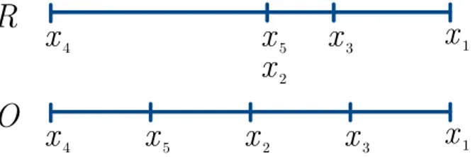
Example 4. The fuzzy ranking � = (�4 ≫ �5 ≈ �2 ≥ �3 >�1) defined on � = {�1, … ,�5} states that, according to expert’s opinion, the fourth alternative is much better than the fifth one that, in turn, is similar to the second one, while both are a little better than the third one that, in turn, is better than the first one.
If we look at Example 4, it becomes clear that, by relying on standard ordinal rankings, it would have been impossible for the same expert to specify her belief so thoroughly. In fact, the ordinal ranking �4 ≻ �5≻ �2 ≻ �3 ≻ �1 that can be extracted from R and can be summarized with the ordering array � = (5, 3, 4, 1, 2), has a deeply different semantics: ties are not allowed so the equivalent alternatives �5 and �2 are artificially ordered while the preference gaps between �4 and �5, �2 and �3, �3 and �1 seems comparable in O while they are very different in expert’s belief, as expressed in R.
Figure 5 graphically illustrates the interpretation of the expert’s belief captured by the fuzzy ranking R of Example 4 and by the extracted ordinal ranking �. As it can be seen, fuzzy rankings offer more tools to highlight the differences between alternatives with respect to ordinal rankings. Inspired by studies on the use of linguistic labels in GDM like [47], the cardinality of S (i.e. the number of available symbols) has been chosen small enough so as not to impose useless precision to the experts and rich enough to allow a
discrimination of the relative performance of the alternatives. On the other hand, the possibility to compose fuzzy rankings by chaining alternatives and symbols, allows to indirectly express a wide variety of preference levels.
Figure 5. Interpretation of the fuzzy ranking R coming from Example 4 and of the extracted ordinal ranking O
As an option, experts may be allowed to provide multiple fuzzy rankings interesting disjoint subsets of X, rather than just one. In this way it is possible to deal with the case in which some options are considered as mutually incomparable. As for ordinal rankings, conversion algorithms to and from FPRs can be defined for fuzzy rankings, as well as similarity measures. Such methods are described in the next subsections.
2.3 From Fuzzy Rankings to FPRs
Starting from a fuzzy ranking � = (�𝜎(1) �1 �𝜎(2) … �𝜎(𝑘−1) �𝑘−1 �𝜎(𝑘)) it is possible to generate the corresponding FPR � = (�𝑖𝑗) in several ways. A first approach consists in associating a predefined preference degree �(�) to each symbol � ∈ � and obtain FPR elements from R in this way:
• �𝜎(𝑖)𝜎(𝑖+1)=�(�𝑖) ∀� ∈ {1, … , � − 1}; • �𝜎(𝑖+1)𝜎(𝑖)= 1− �(�𝑖) ∀� ∈ {1, … , � − 1}; • �𝜎(𝑖)𝜎(𝑖)= 0.5 ∀�{1, … , �}; (32)