Scuola di Ingegneria dell’Informazione
POLO TERRITORIALE DI COMO Master of Science in Computer Engineering
Active Noise Control: a case study
Supervisor: Prof. Fabio Salice
Assistant Supervisor: Prof. Luigi Piroddi
Master Graduation Thesis by: Giacomo Laita Student Id. number: 754404
Scuola di Ingegneria dell’Informazione
POLO TERRITORIALE DI COMO
Corso di Laurea Specialistica in Ingegneria Informatica
Controllo Attivo del Rumore:
un caso di studio
Relatore: Prof. Fabio Salice Correlatore: Prof. Luigi Piroddi
Tesi di laurea di: Giacomo Laita Matricola: 754404
List of Figures 12
List of Tables 14
List of Algorithms 16
Introduction 19
1 Active Noise Control 24
1.1 Algorithms for ANC . . . 26
1.2 Operative principles . . . 28
1.3 ANC concept extension . . . 31
2 The Literature 33 2.1 Duct arrangement . . . 33 2.2 Fan improvement . . . 39 2.3 Fan modeling . . . 56 2.4 Others . . . 60 2.4.1 Applications examples . . . 65
2.5 Summary and key ideas . . . 76
3 The proposed method 78 4 Measurements and Modeling 85 4.1 Experiment setup . . . 86
4.2 DVB-T device power model . . . 90
4.2.1 Data preprocessing . . . 96
4.2.2 Power model . . . 102
4.2.3 Results and Model selection . . . 109
4.3 Speaker power model . . . 115
4.4 Model matching . . . 123
1.5 Example of the superposition principle . . . 30
2.1 Dual ANC system setup . . . 34
2.2 SPL vs. airflow of a fan with and without the duct . . . 34
2.3 Narrow band noise spectrum with ANC system off and on . . . 35
2.4 Acoustic system used . . . 36
2.5 Implementation results of the fan noise power spectrum . . . 36
2.6 A dipole source in a side branch resonator . . . 37
2.7 Experimental setup . . . 38
2.8 Frequency spectra of ventilating fan noise and residual noise at error microphone position; with switched off ANC system (thick lines) and with switched on ANC system (thin lines); black lines for the SBR secondary source and gray lines for the classical monopole source . . . 38
2.9 On-axis far-field sound-pressure level from the shaken fan unit relative to the BPF tonal sound-pressure level radiated by the same fan in free-delivery operation. The independent variable is the apparent electrical power supplied to the mechanical shaker . . . 39
2.10 Directivity condition analysis . . . 40
2.11 Experimental setup used to demonstrate active fan noise control. . . 40
2.12 Spectra of the fan sound-pressure level sensed at the error sensor position, when the controller is on and off. . . 41
2.13 Sound power level reduction in a baffled axial-flow fan as a function of frequency (dB) . . . 41
2.14 Sound-pressure level directivity patterns measured for the baffled fan with the small flow obstruction in position, with and without the ANC in operation . . . 42
2.18 Magnetic bearings control system . . . 44
2.19 Block diagram of magnetic bearings system . . . 44
2.20 Block diagram of the ANC system: the reference signal x(n) is generated by a tachometer on the fan motor, u(n) is the noise control signal, y(n) is the anti-noise one and d(n) is the radiated fan noise which depends on the BPF . . 45
2.21 Experimental setup . . . 46
2.22 Spectra of sound pressure level (76.5 Hz) . . . 47
2.23 Spectra of sound pressure level (100 Hz) . . . 47
2.24 Experimental setup to study the acoustic radiation, resulting from the rotor and the upstream obstruction . . . 48
2.25 Picture of the rotor/stator arrangement . . . 48
2.26 Sound pressure spectrum with (black thick line) and without sinusoidal flow ob-struction (gray thin line) . . . 49
2.27 Resonator location . . . 50
2.28 Superposition of fan and resonator sources . . . 50
2.29 Mouth patterns. . . 51
2.30 Outer fan shroud with relevant dimensions (mm) . . . 52
2.31 Blade passage frequency level, together with the level of each harmonic at half of the velocity loading condition . . . 52
2.32 Mouth perforated patterns, tested in experimental noise reduction model . . . . 53
2.33 Blade tone SPL reductions with optimized resonator mouth perforation . . . . 53
2.34 Phase-locked loop block diagram . . . 54
2.35 FFT spectrum of the pair of fan with dominant tone at 350 Hz . . . 55
2.36 SPL comparison . . . 57
2.37 Sound measurement setup . . . 57
2.38 Sound power comparison . . . 59
2.39 ANC system employing the input separation . . . 60
2.40 Acoustic measures of the different components fans . . . 62
2.41 Fans and sensors location . . . 63
2.42 Dynamic fan control: implementation . . . 63
2.43 Dynamic fan control: control curve . . . 64
2.44 Control results . . . 64
2.45 Data projector (a) and controller block diagram (b) . . . 65
2.46 Pick-up microphone locations . . . 67
2.47 Controller block diagram, together with delay blocks relocated in series with transfer functions . . . 67
2.48 Results . . . 68
2.49 The increase of the vent holes number . . . 69
2.50 Other modifications . . . 70
2.51 Noise spectrum comparison . . . 71
4.5 Example of the measurement setup . . . 90
4.6 Example of the measurement setup: zoomed detail . . . 90
4.7 Schematic of the microphones position . . . 91
4.8 3D points disposition . . . 94
4.9 Points dispositions . . . 95
4.10 Points connections: global view . . . 98
4.11 Points connections: upper view . . . 99
4.12 Deleted points after the processing . . . 100
4.13 Fans noise: frequency analysis . . . 101
4.14 Device and ideal sources (upper view): the values indicate the strengths of the sources . . . 114
4.15 Genelec 6010A . . . 115
4.16 Genelec 6010A: frequency response and polar pattern . . . 116
4.17 Spherical coordinates . . . 118
4.18 Measuring gear: loudspeaker . . . 119
4.19 Loudspeaker model points (blue) and excluded ones (red). . . 120
4.20 Loudspeaker acoustic center (red symbol) and ideal sources (blue points). . . . 122
4.4 SET-UP: sampling distances along y and z-axis (m) . . . 93
4.5 Brute force approach: results . . . 109
4.6 Results for M = 1 . . . 110
4.7 Heuristic approach results for M = 2 . . . 110
4.8 Heuristic approach results for M = 3 . . . 111
4.9 Heuristic algorithm: medians of the classes residues . . . 111
4.10 Heuristic algorithm: W CF results . . . 113
4.11 Final model information . . . 113
4.12 Polar pattern test . . . 117
4.13 Microphones array: microphones distances (Loudspeaker case) . . . 119
4.14 Sampling distances along z-axis, with array aligned with the x-axis (Loudspeaker) 120 4.15 Heuristic algorithm: WCF computation results (loudspeaker) . . . 121
4.16 Loudspeaker final model . . . 121
4.17 DVB-T device: final model . . . 123
4.18 Loudspeaker: final model . . . 123
4.19 Heuristic algorithm: W CF computation results (Model matching) . . . 126
4.20 Matching first solution . . . 126
4.21 Matching second solution . . . 126
8 Heuristic algorithm: SELECTION block . . . 108
The master thesis here presented is part of the project PIANO (the Italian acronym of “low cost platforms for the active noise control”) which was commissioned to Politecnico di Milano in February 2011.
The project goal is the attenuation of the noise produced by two high rotational cooling fans of a Digital Video Broadcasting - Terrestrial (DVB-T) device.
In order to adopt a pervasive solution, it is necessary to employ a hardware-implemented Active Noise Control (ANC) methodology: this utilizes electro-acoustic sensors and actuators to generate an anti-noise signal, whose aim is the cancellation of the disturbance in a particular point in space (quiet zone).
Nevertheless, the project specifications prohibit any structural modification of the device, with the exception of small microphones and loudspeakers installations, provided that the cooling performance is not damaged. A dedicated study is needed to built a robust method for defining the correct actuators number and positions, in order to achieve the project goal as well as to extend the quiet zone.
The description of the selected method is presented after a state of the art analysis: this method is based on the assumption that the power, measured in a point, could be expressed as the sum of the ones generated by ideal sources located near the device. Once a 3D point grid is defined, acoustic measures on it allow the computation of the model for the two fans; then, the actuator one is obtained by adopting a similar procedure.
After that, the optimal number and positions of loudspeakers are derived itera-tively from the above models: hence, it is possible to have the best combination of actuators to reproduce the original energy field.
di controllo attivo del rumore (ANC) implementata in hardware: essa utilizza sensori ed attuatori elettroacustici per la generazione di un segnale di cancellazione, atto ad attenuare il disturbo in una particolare zona dello spazio, detta zona di quiete.
Le specifiche di progetto, tuttavia, vietano qualsiasi modifica strutturale del dispo-sitivo ad eccezione dell’installazione di piccoli microfoni ed altoparlanti, purchè questi non compromettano le prestazioni. Si è quindi costretti a sviluppare uno studio dedi-cato alla costruzione di un metodo per definire il numero e le posizioni ottimali degli attuatori, permettendo non solo di raggiungere l’obiettivo ma anche di estendere la zona di quiete.
Ad una prima parte che si focalizza sull’analisi dello stato dell’arte, segue la descri-zione del metodo adottato: esso si basa sulla costrudescri-zione di un modello che consenta di esprimere la potenza, misurata in un punto, come la somma di quelle generate da un numero predefinito di sorgenti ideali, localizzate in prossimità del dispositivo.
Tale modello viene calcolato per le ventole grazie ad acquisizioni acustiche su una griglia tridimensionale di punti; similmente, la procedura viene adottata anche per ricostruire il modello dell’attuatore.
Dopo aver così ottenuto i modelli, si procede iterativamente per ricavare il nu-mero e la posizione ottima degli attuatori, in modo da riprodurre al meglio il profilo energetico originale.
The PIANO project
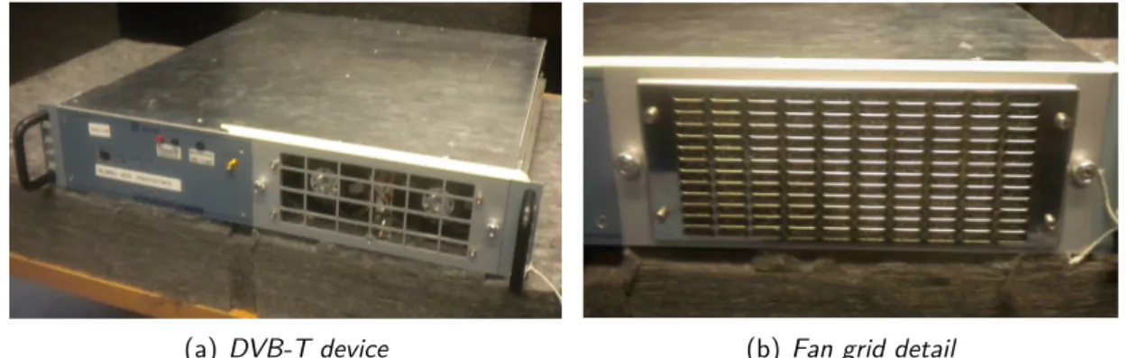
The PIANO project goal is the reduction of the noise emitted by two high perfor-mance cooling fans of a DVB-T (Digital Video Broadcasting Television) elaboration system (Fig.1): this type of fan reaches high rotational speed, that aims at dissipat-ing the high amount of heat released by the image processors, in order to keep the computational performance requirements unchanged.
(a) DVB-T device (b) Fan grid detail
Figure 1: Device under study, kindly provided by SY.E.S.
Furthermore, these devices are organized in racks and placed inside a closed room: it is easy to understand how much annoying the generated global noise can be for an operator who has to work nearby.
that it does not affect the cooling performance and the possibility of performing main-tenance: thus, the noise reduction system must be embedded into the device. All these restrictions forced the adoption of a hardware (FPGA) implemented ANC sys-tem, while acoustic sensors and actuators, as microphones and loudspeakers, were chosen.
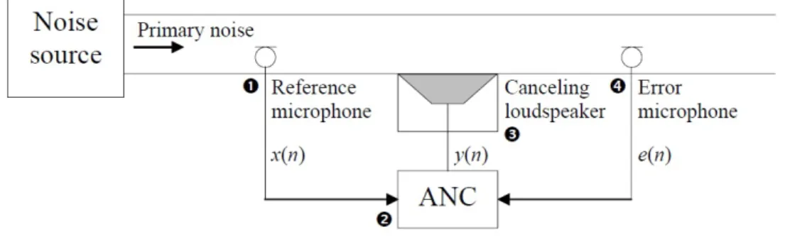
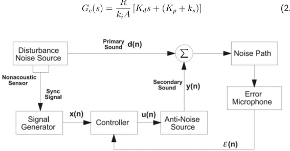
Figure 2: A Basic ANC scheme
Briefly, a basic ANC system, shown in Figure 2, has to sense and then elaborate a reference signal coming from the operating environment: in most of the cases, this last signal is the same of the noise or a quantity related to it. By having this infor-mation, the controller is able to generate the attenuation signal. Since the procedure is designed to eliminate the disturbance in a well established area (quiet zone), an error sensor needs to be placed there (even if this is not always possible): therefore, its measures are used as performance hints and fed to the elaboration section. An algorithm, typically an adaptive LMS (Least Mean Square) one, updates the coef-ficients of a control filter whose output drives the canceling actuators, after being properly manipulated: the filter weights the reference signal upon the performance information given by the error sensor.
Obviously, this thesis work does not cover the entire project: in fact, the ANC controller issue has already been discussed in [12] and [10]. The first paper presents an exhaustive description of the algorithm choice: after having compared different LMS algorithmic solutions, the FxLMS (Filtered-x LSM) was the one adopted. The authors describe also the translation of the general equations of the method into a hardware language and the algorithm implementation on a FPGA board. [10] deals with the hardware problems and the adopted solution to accomplish a good implementation and a good computer-controller communication. Please, refer to the cited papers if additional information is needed.
if such a specific problem has already been addressed by the scientific community. After that, the work will proceed in Chapter 3 by illustrating the adopted method to extend the quiet zone. Chapter 4 will deal with the method implementation in order to compute the fans model as well as the control source one: this chapter will end with the matching between the two models and the analysis of the results.
Acoustic noise is sound which is perceived as “offensive” when heard [26]. Several different types of sources can produce this kind of disturbance: for instance, large in-dustrial equipments, household appliances, transportation equipments and electronic devices. The growing attention to the problem, from both the legislative and the acoustic comfort perspectives, has forced the scientific community to develop inno-vative and cost-effective noise control strategies.
The whole set of possible solutions can be divided into passive and active methods: the first category reduces the noise by absorbing it, through the employment of passive structures like barriers, silencers, mufflers and different types of absorbing materials. Although these systems have the ability of attenuating a broad range of frequencies, they are large, costly and ineffective at low frequencies. On the other side, the Active Noise Control (ANC) employs electro-acoustic systems to cancel the unwanted noise through the addition of sound, according to the superposition principle and three physical mechanisms: destructive interference by way of creation of an anti-noise signal (Fig.1.1), impedance coupling and acoustic energy absorption.
The “actors” of an ANC system, from a control systems perspective, are:
• the plant, i.e. the physical system to be controlled (the DVBT device in this case of study);
• the sensors, to sense the disturbance and to monitor how well the system is performing (microphones);
• the actuators, the devices which do the work of altering the plant response (loudspeakers);
• the controller, that is, the signal processor which tells the actuators what to do, on the basis of sensors’ signals and the knowledge of how the plant responds to the actuators (FPGA).
Figure 1.1: Destructive interference example
Active control systems are able to operate at low frequencies, where passive meth-ods are ineffective: moreover, the reduction is achieved without physical modification or rearrangement of existing noise sources. Additional benefits also include: increased material durability and fatigue life, lower operating cost, compact size and modularity. On the other hand, one of the major limitations of these systems is that the reduction of noise, in a localized specific region, has the unwanted side effect of amplifying it elsewhere: in addition, the noise to attenuate needs to be measured before it reaches the area of interest.
Figure 1.2: LMS block diagram
The most common adaptive algorithm is the Least Mean Square (Fig.1.2): it is able to identify a filter, whose a-priori impulse response h(n) is unknown, by the approximation of a secondary filter, W (n). The convolution theorem states that
d(n) = h(n)∗ x(n) (1.1)
and
y(n) = w(n)T ∗ x(n) (1.2)
with the algorithm filter weights estimation w(n) based on the previous values of x(n), inside a predefined window
w(n) = [w1(n), . . . , wL(n)] (1.3)
x(n) = [x(n), . . . , x(n− L − 1)]T (1.4)
In order to estimate the w(n), the function to minimize is simply
J (n) = E| (d(n) − y(n))2| (1.5)
The resolution uses the derivative operator and then sets to 0 the results to obtain the following weights update rule
wl(n + 1) = wl(n) + µx(n− l)e(n), for l = 0, 1, . . . , L − 1 (1.6)
This simple algorithm has its own limitations, which are overcome by the FxLMS (Filtered-x LMS), as represented in Figure1.3.
The basic innovation is the introduction of the block function S(z), which de-scribes the effect produced on the attenuation signal by:
Figure 1.3: FxLMS block diagram
• the acoustic channel between the actuator and the cancellation area and the one between this area and the error microphone.
The error equation changes by adding the secondary path estimation
e(n) = d(n)− (s(n) ∗ y(n)) (1.7)
First of all, the secondary path needs to be estimated off-line by injecting, for example, a white noise into the loudspeaker in order to measure the path impulse response ˆ
s(n). Since the error microphone signal is used to update the filter coefficients, the condition of no noise in the primary path should be satisfied. Hence, a first equation for the weights update is built
ˆ
sl(n + 1) = ˆsl(n) + µx(n− l)e(n), for l = 0, 1, . . . , L − 1 (1.8)
Thus, the revised filter update equation becomes
wl(n + 1) = wl(n) + µx′(n− l)e(n) (1.9)
x′(n− l) = −ˆs(n) ∗ x(n) (1.10)
The insertion of a further estimation block may cause an increasing of the error and, at the same time, instability may arise too. To avoid this, the gain µ must be restrained and the phase error between s(n) and ˆs(n) has not to exceed 90◦.
the ANC system must be adaptive [21]: this means that a reference microphone must sense an input signal, which should be highly correlated to the primary noise. Moreover, this signal should be fed to the elaboration section, for generating the anti-noise signal which has to reach the desired quiet zone before the disturbance [26]. This issue involves the analysis of the buffering problem, which implies the synchronization of the elaboration section in order to drive the secondary source with the correct signal at the correct time (in relation to this project, [10] solved the problem of signal buffering).
The positioning of the reference sensor near the device, so that it is possible to acquire such a good reference signal, should not be a difficult task. Moreover, the faster the elaboration system is, the closer the secondary source can be placed to this reference microphone, by paying attention to the possible interaction between the noise and anti-noise signals (feedback problem). Considering the use of a small and easily mountable actuator, the control source could be located in the proximity of the device: however, the main problem still remains the location of the error microphone. Acoustically speaking, sound is a pressure wave traveling in a medium, at high speed too. The sound emitted from a source becomes less loud as it goes away from its origin, because the initial energy is spread out over an increasingly large area. It’s a well-known theory that, if a waveguide is present (like a duct), sound can travel long distances without significant decay.
So, let’s focus our attention on image 1.4: a disturbance is passing through a control volume of a tube with cross-section S and length dx, whereas p and ρ denote the pressure and density variation respectively. The 1-dimensional wave equation can be described by using the mass and the momentum conservation laws: this equation explains how the acoustic pressure fluctuations behave with respect to time and space
∂2p
∂x2 −
∂2ρ
∂t2 = 0 (1.11)
If an adiabatic acoustic compression takes place, p = c2
0ρ and so ∂2p ∂x2 − ∂2p c2 0∂t2 = 0 (1.12)
The last equation is linear and contains only differential operators: the solutions are in the form of p(x, t) = f (t− x/c0) for the forward traveling direction and
p(x, t) = g(t + x/c0) for the backward one. The linearity involves also that the
superposition principle p(x, t) = p1(x, t) + p2(x, t) applies to the equation solutions
and, thus, the active noise control principle can be applied in practice. In fact, by considering harmonic waves, the equation is reduced to
p(x, t) = ℜ[p(x)ejωt] (1.13)
= |A| cos(ωt − kx + ϕA) (1.14)
where ω = 2π/T is the angular frequency and k = 2π/λ the wave number. The superposition principle, considering harmonic waves traveling in the same positive direction, can be expressed as
p(x) = Ae−jkx+ Be−jkx (1.15)
If an equal amplitude reverse phase sound wave can be generated, it ends with Ae−jkx for the noise signal and −Ae−jkx for the anti-noise one
p(x) = Ae−jkx− Aejkx = 0 (1.16)
Figure1.5expresses the relation above: the red line is the pressure emitted by the noise source, while the blue one is the pressure from the secondary source (e is the position of the loudspeaker). The error microphone is placed where it’s desired that the attenuation occurs (point L). By detecting the waves’ difference (Fig.1.5(a)), the system is able to adjust the amplitude and phase of the control one to achieve the complete attenuation of both sounds (Fig.1.5(b)).
An important remark arises: the global attenuation can be obtained only if both waves generate a comparable pressure profile at the area of interest. This means that the pressure must be uniform in a direction normal to the propagation one: if this happens, the wave can be called plane waves.
(b) Operating point situation
Figure 1.5: Example of the superposition principle
The duct helps the attenuation process due to its ability of attenuating the prop-agation of high order modes, which quickly decay with the distance thereby allowing the propagation of plane waves at sound speed: anyway, this case of study has no duct and, as stated in the introduction, the project specifications clearly compel to avoid the addition of hardware that could limit the operator work.
The above dissertation is still valid if the condition of far field holds: this is the sound field in which sound pressure decreases inversely with the distance from the source; it corresponds to a reduction of approximately 6 dB for each doubling distance. The acoustic condition of far field can be expressed as
dF arF ield ≫ λ =
c0
f (1.17)
which, considering low frequency disturbance, is equivalent to meters. This is a problem, because it implies that the error microphone should be positioned inside the forbidden region.
1.3 ANC concept extension
In summary, the main limitations, imposed by the ANC on the project goal, are two: the placement of the error microphone in the forbidden region and the need of extending the quiet zone to optimize the overall attenuation.
This master thesis proposes its own solution, which involves the use of a standard noise control methodology, aided by experimental studies, in the direction of the smart placement of sensors and actuators: in particular, the solution is based on the mathematical modeling of both the noise generated by sources and the anti-noise by the actuators. Once a model is available, it is possible to search the best loudspeakers position to achieve the established goal.
In order to develop such a method, it is important to carry out a state of the art analysis in order to understand if this problem has already been addressed by the scientific community: hence, the next chapter is dedicated to this aim.
The Literature
An initial state of the art analysis, which was carried forward until October 2012, is here presented. The investigation was aimed at understanding if this particular kind of problem has been already addressed in research works and also how it has been solved. The papers revision allows the definition of four majors classes of works, which are described in the following; after that, a final and global evaluation is pro-posed.
2.1 Duct arrangement
As it was already stated, the standard ANC systems perform to the best of their ability if the problem is duct “driven”: so, it’s no accidental that a lot of jobs deal with this type of issue.
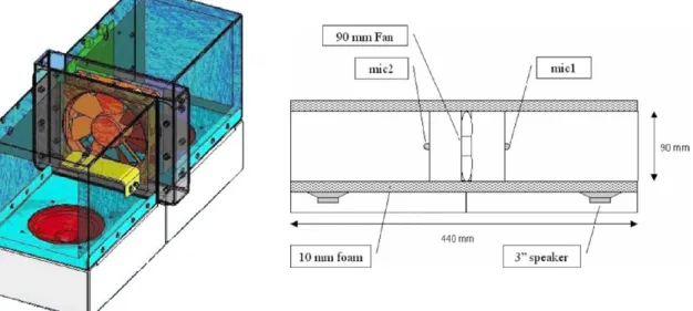
The use of a duct has the disadvantage of requiring extra volume and of con-taminating the system, but the acoustic field composition of fan and loudspeaker is simplified and, by lining the duct with acoustic foam, the high frequency disturbances are attenuated. These statements are underlined by [1], whose authors conclude that the better the primary and secondary source directivity is in agreement, the better the control is. [5] proposes a combination of passive and active noise control to at-tenuate the noise produced by a 90×90×20 mm fan positioned at the midpoint of a 440 mm-long duct, whose cross-section is designed to avoid obstructing the airflow, thereby not lowering the cooling performance.
Each part has the same, but independent, ANC system running: the gear is composed by a loudspeaker, a reference microphone placed 3 cm away from the center of the fan and an electronic controller Figure 2.1.
Figure 2.1: Dual ANC system setup
The choice of the latter one relies on a Silentium’s S-Cube™ controller running an FxLMS algorithm: an interlaced Echo Cancellation algorithm is added for taking care of the echo issues, due to the fact that each microphone picks up signals from both loudspeakers. After establishing the operating point of the fan (see [5] for further details) the attenuation performance is evaluated.
Figure 2.2: SPL vs. airflow of a fan with and without the duct
Figure2.2 shows that the use of a duct passively attenuate the noise SPL, while the performance, see Figure2.3, validates the proposed method in noise attenuation at low frequencies.
Figure 2.3: Narrow band noise spectrum with ANC system off and on
In their paper [33], Sebald and Veen explain that the adoption of a duct causes the air turbulence to contaminate, due to pressure fluctuation, the reference microphone measures and so to degrade the performance of a noise remover. A smart placement of the microphone can help to overcome the problem: a most effective discrimination can be achieved by placing the sensor parallel to the air flow.
In [6] Fleming et al. introduce a new technique for controlling low-frequency reverberant sound-field without the need of a precise plant model. They state that once the interaction between sound-fields, mechanical speaker and electromagnetic transducer is known, a simple electrical impedance can be designed and connected to the terminals of a loudspeaker in order to alter its dynamic and improve the dissipation of the acoustic energy. The impedance is then connected to an electrical network, which is designed on the electrical properties of the loudspeaker to make it emulating the acoustic response of a Helmholtz resonator: in this way, highly resonant acoustic modes can be attenuated. Due to the narrow-band nature of this type of resonators, the obtained acoustic mitigation is highly dependent on the target acoustic resonance frequencies.
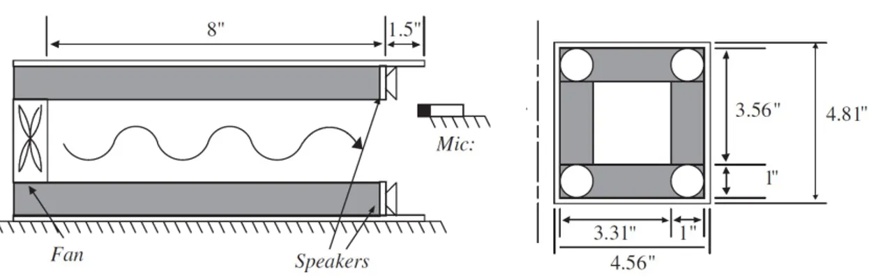
[9] plans an optimal internal model-based (IMB) controller in order to attenuate the noise coming from a rack server cooling fan: the aim is to reduce the periodic acoustic disturbances in presence of a non-periodic ones. To accomplish this mission the rack is mounted inside a duct lined with acoustical foam: four speakers are connected in parallel and placed at the end of it near to the pick-up microphone2.4.
Figure 2.4: Acoustic system used
The controller, after its design (see [9]) and the identification of the sensors and disturbance dynamics, is tuned to match the resonance modes of the system. The results are shown in Figure 2.5 and a good attenuation is achieved, despite a little amplification of sound near the first four harmonics due to the sensitivity of the IMC Bode’s diagram.
(a) IMB off
(b) IMB on
[27] implements a feed-forward active noise control system which combines a single loudspeaker, that acts as a dipole secondary source, with a side branch resonator to reduce the acoustic feedback. The basic idea is that two monopole sources, with appropriate signal delay τ0 = L/c0 (where L is the length of the side branch resonator
and c0is the sound speed), form an unidirectional sound source in a duct if, and only if,
they have same amplitude but reverse phase: the sound generated on the back side of the loudspeaker is used for acoustic feedback reduction. Literally speaking, the sound formed on the other side (front of the loudspeaker), which propagates upstream, is canceled by the sound generated on the rear side. An acoustical short circuit is employed for acoustic feedback reduction and the side branch resonator (SBR) acts like a transmission line for frequency response improvement of the secondary source in band pass frequency range. Also dipole, as a typical loudspeaker is, can be used for such a reduction: a lot of care has to be paid to the acoustic geometrical setup.
Figure 2.6: A dipole source in a side branch resonator
A simple analysis is performed on the various sound fields in the pipe (they are represented by the pi in Figure 2.6), with the purpose of finding their amplitude
coefficients and determining the boundary conditions at the SBR openings (gray points). It comes out to the authors’ attention that the shorter the side branch resonator is, the higher is the central frequency of feedback reduction and the broader its useful frequency range. Besides, the volume flow generated on the backside of the loudspeaker cone is distributed across SBR cross section A2, while the flow at the opposite is distributed in two directions of the main duct 2A1: as a consequence, the sound pressure created in the upstream direction is proportional to 1/A1, whereas the one in the downstream direction to 1/A1 + 1/A2. It can be pointed out that the higher is the ratio A1/A2, the better is the feedback reduction. Hence, the first scheme has to change as Figure 2.7 shows: the length of the SBR is shorter and the cross section ration is set to 1.
Figure 2.7: Experimental setup
Measurements are performed and a pink noise excitation is fed to the system, in order to:
• find out the whole set of acoustic paths needed to apply the active noise re-duction algorithm FxLMS ;
• understand how the dumping material, inside the SBR, can affect the directivity of the secondary source.
The application of this new method ensures a faster convergence and a lower level of residual noise. If the SBR secondary source is switched off, attenuation can be pursued despite a 3dB insertion loss, due to the dumping material: by the way, it is fundamental for obtaining the directivity which is necessary to reach the wanted feedback reduction (Fig.2.8).
Figure 2.8: Frequency spectra of ventilating fan noise and residual noise at error microphone position; with switched off ANC system (thick lines) and with switched on ANC system (thin lines); black lines for the SBR secondary source and gray lines for the classical monopole source
2.2 Fan improvement
Lauchle et al. [13] take under consideration the problem of attenuating a noise coming from a discrete-frequency axial-flow fan and propose a very interesting and innovative method. First of all, this type of fan radiates sound at the blade-passing frequency (BPF), whose value is given by the number of fan blades multiplied by the shaft speed: the predominant direction of radiation is 90◦ to the fan axis.
The smart idea is to use the fan itself as an anti-noise source by connecting it to an electromagnetic shaker to generate controlled unsteady forces on the primary source.
If the shaken fan unit produces substantial radiation for a reasonable power input to the shaker and the fan noise directivity patterns (of the primary and secondary sources) are identical, thus the method is implementable. Experiments show that the first condition is satisfied by suppling 0.1 W to the shaker (Fig.2.9): furthermore, the image suggests that the shaken fan can act as a crude loudspeaker, thereby being suitable for ANC applications.
Figure 2.9: On-axis far-field sound-pressure level from the shaken fan unit relative to the BPF tonal sound-pressure level radiated by the same fan in free-delivery operation. The independent
variable is the apparent electrical power supplied to the mechanical shaker
The second condition is verified thanks to the experimental setup showed in Figure
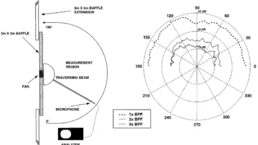
2.10(a): a movable microphone, placed in the free-field 1 meter far from the fan, provides measurements every 5◦for baffled and unbaffled axial flow fan units. Because of the better pattern uniformity in the baffled case, as it is visible in Figure2.10(b), the performance of the baffled shaken fan in noise reduction is now taken into account: an FxLMS algorithm is implemented and an optical tachometer is used as reference sensor (Fig.2.11).
(a) Experimental setup for
measur-ing baffled fan directivity
(b) Far-field directivity pattern
Figure 2.10: Directivity condition analysis
Figure 2.12: Spectra of the fan sound-pressure level sensed at the error sensor position, when the controller is on and off
Comparing the spectra (Fig.2.12), it is possible to note a reduction of 20 dB for what concerns the fundamental BPF tone, while 15 dB and 8 dB are, respectively, the values for the second and third harmonics.
This harmonics attenuation lowering is caused by to the less uniform fan directivity for higher BPF’s harmonics. Figure2.13allows the evaluation of the power radiated by the fan with and without the activated controller: 13 dB and 8 dB are the reduction of the fundamental and the first harmonic which are lower than the ones at the microphone location.
Figure 2.13: Sound power level reduction in a baffled axial-flow fan as a function of frequency (dB)
Figure 2.14: Sound-pressure level directivity patterns measured for the baffled fan with the small flow obstruction in position, with and without the ANC in operation
This is clearly visible in Figure 2.14, that highlights the obstruction created by the cylindrical rod, placed across the center of the fan during the experiment setup; moreover, the same image shows how much good the attenuation is along the fan axis.
The authors also test the shaken fan in a last experiment: an empty desktop computer cabinet is placed on the planar baffle over the fan, which moves air to the case. The error microphone is positioned inside the cabinet, while a remote one is located 1 meter far from there: this setup leads to a noise reduction of 21 dB at the external position and 26 dB at the internal one.
In conclusion, the new method demonstrates that the fan itself can act as an anti-noise source, avoiding the need of adding a separate secondary source.
Lauchle’s concept is extended one step further by [18], [30], [17] and [29]: instead of connecting the fan to a shaker, the impeller is equipped with magnetic bearings which support it and allow the fan blade to be actuated like an audio speaker, by moving the impeller back and forth (Fig.2.15).
Co-locating the disturbance produced by the impeller rotation and the attenuation signal from the vibration of the fan impeller has the advantage that both signals enter the space in the same point. As [30] states, while trying to demonstrate the effectiveness of the new approach in achieving broadband noise reduction, co-location means also same path; this phrase can be better understood by looking at Figure2.16, which shows the testing gear: the same route length exists both from the anti-noise source to the error microphone and from the disturbance to the same microphone.
Figure 2.15: ANC with magnetic bearings
of broadband noise attenuation, H∞ control theory is adopted [29]. A first analysis shows that the fan impeller, supported by magnetic bearings both radially and axially, generates a broadband and tonal noise, with significant tone at the rotation frequency and at the blade pass frequency (BPF). The authors derive a state space model (nominal plant) for the acoustic system in Figure 2.16: they start from an infinite dimensional physical model by using a subspace algorithm on the system’s response to a white noise signal (see [29] for details). The controller design is focused on obtaining a feedback one, which reduces the gain of the close loop system regarding the tone’s frequencies (Fig.2.17): based on the nominal plant, a single weighting filter is chosen to shape the gain. This has to be greater than the one at BPF, to achieve a significant roll off at high frequency by avoiding an excessive spillover. Subsequently, the controller is obtained by solving the RSP (Robust Stabilization Problem) and the complexity is reduced via elimination of the pole/zero cancellation and state reduction.
Figure 2.16: Schematic of a centrifugal fan noise testing facility
Figure 2.17: Close loop system: Gyw is the duct model, Ga the bearing actuator, K the ANC
controller and w the noise disturbance
As already mentioned, a real implementation of an improved magnetic bearings method is presented in [17]. Because of the bearings’ inherent instability, they require a feedback controller (Fig.2.18) which stabilizes and maintains the rotor in a desired position and, as a consequence, dictates the bearings’ dynamic characteristics.
Figure 2.18: Magnetic bearings control system
Despite the magnets are intended to maintain the rotor in a certain position (the rotor levitates in a nominal position), they can also be used to shake it and to achieve sound control with no additional hardware requirements: the shaking movement can be obtained by perturbing the rotor’s reference position signal u(t) intentionally (Fig.2.19).
In particular, the force f (t) generated by the bearings electromagnets is a function of the rotor displacement z(t) and the winding current i(t), with constants ks as the
force-displacement factor and ki as the force-current one. The transfer function
(Gb(s)), which describes the interaction between bearings and rotor, is so governed
by Newton’s second law and by considering the rotor like a rigid body with mass m. Hence, it follows f (t) = ksz(t) + kii(t) = m d2z(t) dt2 (2.1) Gb(s) = Z(s) I(s) = ki/m s2− (k s/m) (2.2) Ge(s) represents the transfer function for the coil dynamics: by stating that A
is the power amplifier gain, L and R are respectively the coil inductance and resis-tance and, recalling the equations for an electromagnetic coil, the transfer function is expressed as
Ge(s) =
A/L
s + (R/L) (2.3)
The last transfer function, Gc(s), governs the controller position and it stabilizes
the magnetic bearings: proportional-derivative (PD) and proportional-integral deriva-tive (PID) laws are typically used, with constant Kp and Kd as the desired stiffness
and damping, respectively.
Gc(s) =
R kiA
[Kds + (Kp + ks)] (2.4)
Figure 2.20: Block diagram of the ANC system: the reference signal x(n) is generated by a tachometer on the fan motor, u(n) is the noise control signal, y(n) is the anti-noise one and d(n)
is the radiated fan noise which depends on the BPF
Figure 2.21: Experimental setup
The experimental apparatus is visible in Figure 2.21 and it consists of a three-bladed fan connected to a servomotor by a flexible link passing through the supporting magnetic bearings. An error microphone is placed 36 cm in front of the outlet side of the fan, with an 8 cm offset from its rotational axis.
Three experiments are performed in order to demonstrate if the proposed method is capable of generating a sound of sufficiently high amplitude and coherent frequency: this sound should reduce the noise at the error microphone (feedback) and in other points far from it (without the feedback information).
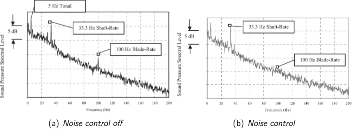
Figure 2.22 shows the noise produced by the uncontrolled situation measured when the fan rotor runs at 2000 rpm: a spike at 100 Hz (corresponding to the BPF) appears on the spectra. If the magnetic bearings are driven by a set of sinusoids (76.5 Hz) with the aim of vibrating the fan only in the axial direction, a spike appears at the given frequency: this spike is the demonstration that the bearings are able to produce sound at a specific frequency.
(a) Noise control off (b) Noise control on Figure 2.22: Spectra of sound pressure level (76.5 Hz)
Further experiments, whose aim is the 100 Hz spike removal (Fig.2.23), illustrate the viability of using magnetic bearings as a noise control actuator. By driving an axial-flow fan with a magnetic thrust bearing, the blade-rate tone of the fan is reduced by 4 dB at the error microphone and by 3 dB at the points which are located at 180 cm far from the error microphone.
(a) Noise control off (b) Noise control
Figure 2.23: Spectra of sound pressure level (100 Hz)
Gérard et al., in their paper [3], provide an analytical tool to design flow control obstructions which destructively interfere with the primary tonal noise arising from cooling fans. Trapezoidal and sinusoidal shapes are suitable for this type of job, since they can control a tone without affecting its harmonics, which is an important issue in the noise control field. The obstruction, as the authors state in [2], must be located so that the secondary radiated sound has equal magnitude but opposite phase compared with the primary noise: in addition, the obstruction should be “location-adaptable” to control non-stationary non-uniform flows. In [2] the experimental setup, which is used to validate the thesis expressed in [3], is shown in Figure2.24: an engine cooling 2.2. Fan improvement
Figure 2.24: Experimental setup to study the acoustic radiation, resulting from the rotor and the upstream obstruction
SPL measurements are done at a BPF of 290 Hz for trapezoidal, sinusoidal and cylindrical obstructions: results reveal that no attenuation is achieved when the ob-structions is at the maximum axial distance between itself and the rotor.
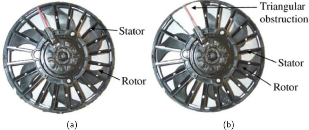
A second set of experiments is tuned to investigate the noise attenuation in the free field. The same setup gear is employed but data are collected with respect to both the couple rotor/stator arrangement (Fig.2.25)(a)) and the rotor/stator plus triangular obstruction, inserted between two vanes of the stator (Fig.2.25)(b)).
(a) (b)
An attenuation of 12.2 dB is achieved in the first case with a small enhancement of the BPF harmonics, thereby proving the frequency selectivity ability of the sinusoidal obstruction. In the second case, same results (10 - 20 dB) are obtained, even if the additional obstruction causes a slight increase of the broadband noise floor (Fig.2.26). It has to be pointed out that this increase is so low to be neglect.
(a) Case 1: upstream
(b) Case 2 upstream
Figure 2.26: Sound pressure spectrum with (black thick line) and without sinusoidal flow obstruction (gray thin line)
Figure 2.27: Resonator location
The resonator is excited when the tip of the blade passes by its perforated mouth, causing a periodic pressure generation: the changing of resonator’s length or mouth opening can originate an out-of-phase condition with respect to the blade tone. In particular, a quarter-wave resonator radiates as a monopole source, while axial fans as dipole source. This resonator can be tuned to be 180◦out-of-phase from the downstream fan noise, in order to reduce the waveform on this side: of course, the upstream waves are in phase and thus amplified (Fig.2.28).
The amplitude of the resonator response depends on the number of resonators involved: furthermore, the perforated mouth is essential for maintaining an high level of fan efficiency so that an accurate investigation needs to be performed. The above mentioned resonators are 152 mm long nylon tubes with a 60 ml syringe tube inside: the perforated mouthpiece is accommodated at the open end while the close end consists of a movable 127 mm long nylon plunger. The mouthpiece is a piece of a 5.1 mm thick aluminum with the same curvature of the inner radius of the fan shroud. In order to fulfill the attenuation job, the resonator acoustic characteristics (i.e. the impedance with respect to mouth porosity) must be known.
Figure 2.29: Mouth patterns
Different resonator’s lengths and mouth patterns are tested (Fig.2.29) and the SPL vs. the resonator frequency response is measured by calibrated probes inside the tube. Results highlight that a reduction in the open perforated area (pattern 1 to 6) causes a shift of the resonant frequency from 598 Hz to 320 Hz and a reduction of the attenuation factor too: in addition, the resonator behavior approaches that of the closed-closed tube type. This type of data is used to model the closed-end resonator response as a function of the driving pressure by acoustic transmission line theory: the resonator attenuation increases as the mouth porosity decreases. The arrangement is tested thanks to the use of a fan facility: a fluted duct, with upstream and downstream anechoic termination and a 260 mm diameter ten blade automobile radiator fan in the middle.
The outer shroud (Fig.2.30) is made by Plexiglas rings glued together: it is de-signed to accommodate ten evenly spaced resonators around the fan’s perimeter, corresponding to each blade. The resonator tubes are inserted into each of these holes and fitted with plugs when they are not used to attenuate the noise. Tests about different loading fan conditions highlight that, at free-stream velocity of 3.2 m/s (by now it will be considered unchanged), the resonators have a negligible effect 2.2. Fan improvement
Figure 2.30: Outer fan shroud with relevant dimensions (mm)
on the fan performance: in addition, the SPL of the fundamental BPF varies depend-ing on the fan load. The author suggests the need of characterizdepend-ing the pressure, generated on the surface of the shroud by the passing blades, to provide both the tuning of the resonators and their anti-phase cancellation analysis.
Figure 2.31: Blade passage frequency level, together with the level of each harmonic at half of the velocity loading condition
Measurements are taken at each hole for three loading conditions: results in Figure2.31 confirm that the peaks occur at the BPF with also the presence of higher harmonics components. Furthermore, the phase analysis shows the existence of a
between upstream and downstream shroud pressures (180◦).
Figure 2.32: Mouth perforated patterns, tested in experimental noise reduction model
Several mouth perforation patterns are tested to evaluate the best noise reduction attitude,by considering the operative fan velocity equals to half of the maximum one (Fig.2.32). At the beginning, the first pattern is adopted to decide the optimal resonator length to obtain the maximum upstream and downstream SPL reduction (221 mm and 304 mm respectively). Taking into account the downstream case tune, a 12 dB reduction at the BPF tone is achieved.
Further experiments lead to the determination of the optimal perforation: pattern 7 reduces the tonal noise 8 dB more than the fully perforated one as well as the harmonics (Fig.2.33). An increase of 4.7 dB occurs in the upstream direction but without effect on the first harmonic. A detailed analysis reveals that a resonator, mounted near the leading edge of the fan blade, is the most effective in attenuating downstream SPLs and vice versa. In practice, since the most axial fans radiate more strongly in one direction, the overall radiated noise reductions can be obtained by reducing noise in the louder direction while the level, radiated in the other directions, increases only slightly.
Figure 2.33: Blade tone SPL reductions with optimized resonator mouth perforation
number of blades of each fan by the number of rotation per second (in this case, between 1200 and 4200 rpm based on a 1 to 9 V variable control input voltage, which varies the speed). The real speed is measured by a tachometer and, because of the noisy signal characteristics, a bandpass filter is implemented.
Figure 2.34: Phase-locked loop block diagram
The above measurements (frequency vs. control voltage) are used to design a phase locked loop (PLL, Fig.2.34) for locking fans to a constant phase. The general strategy is to allow one fan to run freely (acting as reference) and to phase-lock the other to the first one: this choice not only requires to control half of the sources but it is also adaptive to every change that happens to the reference fan.
The whole set of collected data is used for developing a mathematical Laplace-domain fan model, which is then converted into a phase model in order to control that variable instead of the frequency. The PD (Phase Detector) block in Figure2.34
represents a counting-type phase device, which has to find the difference between the accumulated phases of the two fans; at the same time, it has to generate an output signal representing the phase difference in radiants: a compensator, equipped with an integrator able to absorb the DC component of the error signal, adjusts the trade off between the responsiveness to disturbance and the overall system stability.
The fans under analysis are inside a chassis and a microphone is placed 25 cm far away, pointing to the blowers outputs: some experiments are performed considering
(a) Unsynchronized pair of fans
(b) Synchronized pair of fans with canceling tone
Figure 2.35: FFT spectrum of the pair of fan with dominant tone at 350 Hz
subtractive tones. Figure2.35shows the attenuation of the dominant tone at 345 Hz, by a factor of 2.5. It needs to be pointed out that the optimal phase offset must be manually tuned at the operative location: this can be done by analyzing a real-time spectrum of the activated system and seeking for the offset that best reduces the identified tonal component.
the adopted assumptions and boundary conditions). For what concerns the acoustic noise evaluation, the authors show that the numerical simulation of a LES (Large Eddy Simulation) turbulence model can well predict the acoustic behavior of the fan, supplying useful information to the fan designer.
It is recalled here that the noise produced by a fan can be thought as composed by a broadband part and a discrete part. In particular, the second one is a combination of:
• a BPF frequency and its harmonics; • a shaft frequency and its harmonics.
The latter is the result of asymmetries, in the fan structure, which cause distortion in the flow field and low frequency range noise (anyway, very difficult to attenuate). Considering both the broadband and the discrete parts, new hybrid methods for the numerical prediction of the sound field are available and they can achieve acceptable results; in particular, they provide information helpful to study some acoustic effects like eccentricity, which is usually a result of the slight positioning error of the fan rotor.
In [34], the additional aeroacoustic effect, produced by geometrical asymmetries, is taken under test. Furthermore, symmetric and asymmetric rotating fans are modeled and analyzed: detailed information of the mathematical methods can be found in [34]. The models of the two fans are similar: their difference only consists of the 0.45 mm distance between the geometric center and the rotating one of the asymmetric fan. The SPL measurement is shown in Figure 2.36: it is clearly visible that the asymmetry causes the noise to be on average of 5 dB greater than the other case: thus, the first harmonic is 18 dB higher and the angular symmetry is broken.
Any tiny eccentricities can bring large variation of sound frequency spectrum and it needs to be further studied in order to provide a more detailed and complete information to the modeling procedure.
Hence, the work of [34] can be an integration to the one of [32], because it supplies additional hints on how a fan can be better designed.
(a) Globally (b) Harmonically divided Figure 2.36: SPL comparison
As stated beforehand, the cooling property of the flow created by a centrifugal fan is a basic requirement for most electronic devices such as desktop computers and notebooks. On the other side, fans are the less reliable parts and their frequent failures need to be addressed.
Therefore, [24] proposes the study of the acoustic noise generated by two tandem tubeaxial fans, stacking in this configuration to solve the redundancy issues. Doubling the fans brings to a corresponding doubling of the noise output produced, which has to be added to that one deriving from the airflow interaction. In order to quantify the noise, the fans are suspended in a volume by rubber bands to eliminate any additional source of noise, which could be present in a real electronic device enclosure: moreover, the fans are bolted together so that no free movements are allowed and the spacing between them is filled with washers. A PVC frame (Fig.2.37) is created as control volume and its surfaces are orthogonally scanned to acquire the sound intensity, whose sound power is then derived from in accordance with ISO 9614-2.
Figure 2.37: Sound measurement setup
Fan Size (mm) No. of fan blades CFM@12 V
I 120×38 3 112
II 120×38 7 110
III 80×25 7 35
IV 60×25 7 12
Table 2.1: Test fans specifications
The analysis is divided in two sections that is, noise and airflow measurements. For what concerns the second one, which is not of main interest here, please refer directly to page 337 of [24], while the description of the noise measurements is now further analyzed. It is important to remember that, by suspending the fan inside a control volume, no noise-generating mechanisms are present: thus, if the separation distance between the sources approaches the infinite, the airflow interactions reach a minimum and the radiated sound power becomes close to a theoretical reference value. On the other side, the finite separation distance causes the measured power to be greater than the theoretical one and this difference can be ascribed to the airflow influences: indeed, at zero distance the emission reaches the maximum.
Figure 2.38 shows the sound power of Fan Type I and II: the straight line at the bottom of the left image represents the theoretical reference for a single fan sound power, while the dotted line (in both images) is the reference for two fans; in addition, the square marked line is associated with the open channel configuration, while the remaining with the closed one.
As it can be seen in Figure 2.38, the two channel configurations functions are similar and give close results for small separations, whereas the increase of the fans distance cause greater sound power emission (quantifiable as 5 dB) by the closed channel: anyway, the open channel configuration is 4 - 5 dB greater than the baseline reference, indicating that an interaction between the two flows is present.
(a) Fan Type I
(b) Fan Type II
Figure 2.38: Sound power comparison
The two images give also another information: the comparison of the sound power dependency on separation distance is weaker for Fan Type II, pointing out that also the number of fan blades (3 in the first case, 7 in the other) plays a significant role on noise emission.
In summary, increasing the space between two fans can bring about a total sound power reduction of 5 dB because of less interactions between the two flows; moreover, an open to ambient channel can help to further reduce the emission. It needs to be pointed out that tests are performed considering an isolated fan: indeed, a study has indicated that the noise emission of fan mounted inside a chassis is greater than the emission which would be present with only a fan [16].
control becomes implicit without the use of additional sound sources.
[11] proposes a parallel ANC system implementing the standard FxLMS algorithm. The key idea is to split the input signal into periodic and random components: in fact, since periodic signals are perfectly predictable (through a FFT analysis), a perfect anti-noise signal can be generated for them, resulting in a very high attenuation level.
Figure 2.39: ANC system employing the input separation
The Figure 2.39 shows the above stated idea: the input signal x(n) is separated into its periodic q(n) and stochastic v(n) components. These are fed to appropriate ANC systems whose outputs are filtered by the transfer functions of the electrical and acoustic path from the loudspeaker to the error microphone; then the outputs are compared to the predicted noise coming from the sources to end with the error signal, which allows the tuning of the system.
Considering Γx the noise attenuation level of the input x(n), it can be written as
the energy of the signal to cancel (ξd = ξdq + ξdv because of the independence of
stochastic and deterministic parts), divided by the sum of the energies of the error in its periodic (ξeq) and random (ξev) components. Assuming the perfect cancellation
of the periodic part, the upper bound for the maximum noise attenuation level is: Γx= ξd ξ + ξ = ξdq + ξdv ξ + ξ ≈ ξdq + ξdv ξ = Γv ( 1 + ξdq ξ ) (2.5)
The better performance of the separation method is shown for different numbers of tone in the below Table 2.2
Table 2.2: Performance comparison
The separation principle is also used by [19] to propose an alternative algorithm for the attenuation of a periodic disturbance in the presence of a random one. The authors develop a standard state-space model of the system and use a traditional LTI controller as starting point to design an IMC controller, with two aims: tracking and canceling a periodic disturbance and also coping it with the random one. The internal model needs to capture the relevant properties of the unknown input microphones signal: thus, a model of a periodic signal with time-variant frequency is required. Considering that the estimation and rejection of the disturbance should be done together, the frequency of the period must become a state: this produces a non-linear state space equation (because of the presence of the state variable inside cosine and sine), which forces the adoption of an Extended Kalman Predictor for the estimate of states and frequencies.
the noise instead of attenuating it. First of all, individual component acoustic analysis is performed: results highlight that the higher noise is associated with the memory system (Fig.2.40), and therefore, they suggest implementing the fans management on it.
The authors goal is to lower the rotational speed of the fans by maintaining the cooling requirement. Therefore, temperature sensors are needed but their placement selection is critical, because they have to sense the worst temperature value: to do this task, their are located near the heating sources, so that the temperature is registered before the heat is dissipated by the fans (Fig.2.41).
(a) (b)
Figure 2.41: Fans and sensors location
The real time dynamic fan-control implementation is shown below in Figure2.42: when the components on the board are powered on, the ambient temperature rises around the sensors, which send a signal to the micro-controller; the latter increases or reduces the fans speed with respect to the input data, that is, the sensed temperature and the control curve (Fig.2.43).
Figure 2.42: Dynamic fan control: implementation
Figure 2.43: Dynamic fan control: control curve
The RPM control curve, visible in Figure 2.44, allows to run the fans at different speeds depending on the ambient temperature, by causing a reduction from 6 to 11 dBA with respect to the case of all 3 fans running at 100%. A further 4 dBA reduction can be achieved if the fans guard is re-designed, because of the diminished resistance to the air flow.
2.4.1 Applications examples
A feedforward based active noise controller is implemented by [28] on a NEC LT170 data projector: the system under consideration is shown below (Fig.2.45(a)).
(a) (b)
Figure 2.45: Data projector (a) and controller block diagram (b)
A feedforward compensator F (q) is usually fed by the input signal u(t) coming from a pick-up microphone: its output drives the control speaker to attenuate the noise disturbance η(t).
The objective is the reduction of the performance index e(t), which represents the error signal. In particular, if the sound disturbance is not influenced by the compensation one and the compensator is stable, the following stable map equation can be written
e(t) = W (q) [H(q) + G(q)F (q)] η(t) (2.6)
It leads to the ideal compensator
F (q) =−H(q)
G(q) (2.7)
considering that the acoustic coupling minimization is obtained both by shielding the pick-up microphone and by installing non-invasive small directional speakers at the inlet and outlet grill.
The ideal compensator assumes full-knowledge of the other transfer functions: this aspect involves that it is necessary to find an approximated solution through an output error-based optimization. The block diagram (Fig.2.45(b)) and the error Equation 2.6 help to understand that all the needed transfer functions depend on both the microphones and the speakers positions.
In particular, signals u(t) and e(t) are measured for different positions, with the feedforward compensation off (e1(t) when F (q, θ) = 0) and, once again, with the
air-cooling system off (e2(t)).
The collected data can be used to solve the minimization problem and find the filter coefficients (detailed computations can be found in [28], only the relevant steps are reported here)
e1(t) = H(q)u(t) (2.9)
e2(t) = −G(q) [u(t) + ν(t)] (2.10)
e(t, θ) = e1(t)− F (q, θ)es(t)− F (q, θ)G(q)ν(t) (2.11)
The performance, for a specific pick-up microphone position and considering an absence of noise on the input microphone, is evaluated taking into account
VN(θ) := 1 N N ∑ t=1 ϵ2(t, θ) (2.12)
Hence, it can be derived that
ˆ θ = min θ∈RdVN(θ) (2.13) F (q, θ) = p−1 ∑ k=0 θkq−k (2.14)
Operative setup highlights four possible pick-up microphone locations, as Figure
2.46 shows: (1) in proximity of the bulb, (2) in air flow, (3) in the central part and (4) close to cooling fan. The previously described experiments are repeated for each position, resulting in the following VN(ˆθ) values: (1) 1.4171× 10⁻⁴, (2)
1.7725× 10⁻⁴ (there is a lot of noise at the pick-up microphone), (3) 1.0421× 10⁻⁴ and (4) 1.7282× 10⁻⁴. By fixing the pick-up microphone on the third position and putting the error one 25 cm away from the inlet grid, measures of e1(t) and e2(t) are
gathered and used to estimate a low order IIR filter, which is then parameterized by a 24th order FIR filter.
Figure 2.46: Pick-up microphone locations
In their paper [25], Cordourier and Bustamante assert that the main source of continuous noise, generated by a personal computer, is normally the external cooling fan; thus, a single-channel active noise control system with one reference signal (s(n)), one control signal (q(n)) and one error signal (e(t) to minimize) is proposed.
Figure 2.47: Controller block diagram, together with delay blocks relocated in series with transfer functions
Figure 2.47 describes in detail the presented system: in particular, since a com-puter audio processing is implemented by buffering audio blocks on N samples, if the assumption of periodic tonal disturbance is valid, this buffering delay can be overcome.
besides the overall 40 dB attenuation, it appears clear that the system can not elim-inate the main tonal component at 1270 Hz. A further experiment (Fig.2.48(b)), similar to the previous one but with the addition of a cellphone emitting a synthetic tone at 700 Hz, shows that this last tonal component can be totally removed.
(a) Laptop noise without control (upper left), with
con-trol (lower left) and noise reduction level (right)
(b) Same experiment as above, except the adding of a 700
Hz sinusoid
Hence, the data can identify the inability of the system to attenuate a disturbance which is not strictly periodic: in conclusion, the paper asserts the uselessness of the method for laptop cooling fan noise but, on the other side, its usefulness for periodic case disturbances.
A different electronic device, a plasma display panel television (PDP-TV), is an-alyzed by [22] in order to achieve noise reduction and cooling performance improve-ment. This kind of television employs cells of excited Xeon or Neon to create ultravi-olet light based on a digital signal: this requires from 360 to 600 Watt power and so fans are needed to maintain the temperature below the operating limit. The choice is a 7 blades 120 mm diameter fan, which rotates at 1600 r.p.m. producing an overall A-weighted Sound Pressure Level (OASPL) of 25 dB when unloaded. Without mod-ifying the system, the noise attenuation can be accomplished through the increase of the cooling performance, thereby allowing the r.p.m. reduction and so the noise, as pointed out by [4].
(a) Original rear case (b) Modified rear case Figure 2.49: The increase of the vent holes number
Hence, to reduce the flow-induced noise while maintaining the cooling perfor-mance, flow velocity measurements and visualizations with smoke are performed: results reveal a strong concentration near corners also at low speed, provoking an inefficient operating point and noise because the flow does not intersect the fan.
An equation which could describe the SPL of a fan system can be the following, with Kw as the specific noise level and Q as the system resistance (pressure rise in
the fan)
SP L = Kw+ 10log Q + 20 log ∆P (2.17)
In order to reduce the system resistance, the authors propose:
• increasing the number of vent holes, by the modification of the TV rear case, obtaining a 1.7 dB reduction on the broadband noise (Fig.2.49);
(a) Foam ring duct extension (b) Rounded rear case Figure 2.50: Other modifications
The previous ideas aim at reducing the broadband noise; for what concerns the discrete one (related to BPF), the authors discover that the removal of the strut, attached to the display panel for avoiding its deformation due to heat, can help to reduce the noise by 1 dB.
If the whole set of proposed modifications is applied, a gain of 36% on the flow can be obtained: this performance surplus is exploitable to vary the fan r.p.pm. and assess its effects on the noise (Fig.2.51). In particular, the mathematical connection between r.p.m. and fan noise is described by
SP L = SP Lref + 50log ( RP M RP Mref ) (2.18) Final results show the possibility of decreasing the r.p.m. from 930 to 830: this means to achieve a 6.3 dB noise reduction with even a 10% increased flow rate of the fan, thereby improving the cooling performance of the system.