Pricing-based primal and dual bounds for selected packing problems

(1)

(2)

(3)

UNIVERSITÀPOLITECNICA DELLEMARCHE

SCUOLA DIDOTTORATO DIRICERCA INSCIENZE DELL’INGEGNERIA CURRICULUM ININGEGNERIAINFORMATICA, GESTIONALE E DELL’AUTOMAZIONE

Pricing-based primal and dual

bounds for selected packing

problems

Ph.D. Dissertation of:

Andrea Pizzuti

Advisor:

Prof. Fabrizio Marinelli Curriculum Supervisor: Prof. Claudia Diamantini

(4)

(5)

UNIVERSITÀPOLITECNICA DELLEMARCHE

SCUOLA DIDOTTORATO DIRICERCA INSCIENZE DELL’INGEGNERIA CURRICULUM ININGEGNERIAINFORMATICA, GESTIONALE E DELL’AUTOMAZIONE

Pricing-based primal and dual

bounds for selected packing

problems

Ph.D. Dissertation of:

Andrea Pizzuti

Advisor:

Prof. Fabrizio Marinelli Curriculum Supervisor: Prof. Claudia Diamantini

(6)

SCUOLA DIDOTTORATO DIRICERCA INSCIENZE DELL’INGEGNERIA FACOLTÀ DIINGEGNERIA

(7)

(8)

(9)

Acknowledgments

Although in my academic path this is the third thesis that I compose, actually it is the first time in which I have decided to insert acknowledgements in one of them. This is not meant to be disrespectful for people who have accompa-nied me during the Bachelor and Master courses, nor is caused by the lack of wish to thank them for their unshakable support. Simply, this is the earliest time in which I can feel a kind of sincere emotion (viz. sense of satisfaction) in ending the present route, without losing to the compromise of "you should be touched by the incoming goal". For this reason, even if it could sound exces-sive (or just inappropriate) for a Ph.D. thesis, I want to dedicate few truthful words in acknowledgements.

Firstly, I want to affirm my enormous gratitude for my supervisor Fabrizio. He was a solid and priceless landmark in guiding my research activity since my very first steps into the field of research with my master thesis. Moreover, to me he has always been a lighthouse for his strong and admirable ethic, for which I can only feel the highest of respect and estimation. Finally, and most important, he allowed me to find a path that, even if surrounded by difficulties and uncertainties, I have a sincere desire to continue.

Then, I wish to thank my friends. There is no need to report their names, I know they will naturally understand. Some more than others, each of them supported me since I started my studies at university, when I felt as wandering without a precise reason and questioning about my choices. To you, I owe my (little) serenity, the strength of holding on, love and bonds that go beyond what I ever hoped or deserved. Truly, thank you.

Finally, I want to acknowledge my family. Simply, for everything. Ancona, Febbraio 2020

(10)

(11)

Abstract

Several optimization problems ask for finding solutions which define packing of elements while maximizing (minimizing) the objective function. Solving some of these problems can be extremely challenging due to their innate com-plexity and the corresponding integer formulations can be not suitable to be solved on instances of relevant size. Thus, clever techniques must be devised to achieve good primal and dual bounds. A valid way is to rely on pricing-based algorithms, in which solution components are generated by calling and solving appropriate optimization subproblems. Two main exponents of this group are the delayed column generation (CG) procedure and the sequential value correction(SVC) heuristic: the former provides a dual bound based on the gen-eration of implicit columns by examining the shadow prices of hidden vari-ables; the latter explores the primal solution space by following the dynamic of approximate prices.

In this thesis we focus on the application of SVC and CG techniques to find primal and dual bounds for selected packing problems. In particular, we study problems belonging to the family of cutting and packing, where the classical BIN PACKING and CUTTING STOCKare enriched with features de-rived from the real manufacturing environment. Moreover, the MAXIMUM

γ-QUASI-CLIQUEproblem is taken into account, in which we seek for the

in-duced γ-quasi-clique with the maximum number of vertices. Computational results are given to assess the performance of the implemented algorithms.

(12)

(13)

Sommario

Un ampio insieme di problemi di ottimizzazione richiedono l’individuazione di soluzioni che definiscono un packing di elementi, al fine di massimizzare (minimizzare) la relativa funzione obiettivo. Risolvere all’ottimo alcuni di questi problemi può essere estremamente oneroso a causa della loro comp-lessità innata e le corrispondenti formulazioni intere possono non essere ap-propriate per approcciare istanze di dimensioni rilevanti. Pertanto, il calcolo di bound primali e duali qualitativamente validi necessita della definizione di tecniche ingegnose ed efficaci. Una metodologia valevole consiste nell’impiego di algoritmi basati su pricing, in cui le componenti delle soluzioni sono gen-erate tramite la risoluzione di sottoproblemi di ottimizzazione specifici. Due principali esponenti di questa famiglia sono la procedura delayed column gen-eration(CG) e l’euristica sequential value correction (SVC): la prima fornisce un bound duale basato sulla generazione delle colonne implicite tramite la val-utazione dei prezzi ombra di variabili nascoste; la seconda esplora lo spazio delle soluzioni primali seguendo la dinamica di prezzi approssimati.

In questa tesi ci concentriamo sull’applicazione di tecniche SVC e CG per l’individuazione di bound primali e duali per problemi di packing selezionati. In particolare, studiamo i problemi appartenenti alla famiglia del cutting e packing, dove i ben noti BINPACKING e CUTTINGSTOCKsono arricchiti con caratteristiche derivanti dagli ambienti produttivi reali. Inoltre, studiamo il problema della MAXIMUMγ-QUASI-CLIQUEin cui si cerca la γ-quasi-clique

indotta che massimizzi il numero di vertici selezionati. Risultati computazion-ali sono presentati al fine di vcomputazion-alidare le performance degli algoritmi imple-mentati.

(14)

(15)

List of Figures

1.1 Dotted lines separate each subblock, whose non-zero compo-nents do not share row and column indices with the non-zero

components of other subblocks. . . 7

1.2 SVC flow chart . . . 10

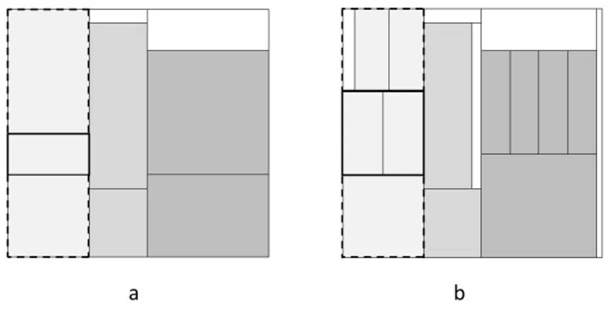
3.1 a) 2-stage pattern; b) (simplified) 3-stage pattern. Dotted lines delimit sections, bold lines highlight the boundary of strips. . . 34

3.2 Dotted lines indicate the potential cuts of the second stage. The bold line refers to the cut closest to the middle of the stock height Hj. . . 39

3.3 sub-pattern pl . . . 39

3.4 sub-patterns pland p′ u . . . 40

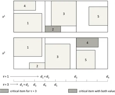
4.1 How the Pareto region changes with τ, ceteris paribus. . . 46

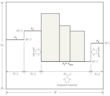
4.2 A skyline, with indication of a roof at minimum quota and of the relevant knapsack; the items in a knapsack solution are ranked by non increasing heights, starting from the highest wall of rmin| in this case, the left one. . . 56

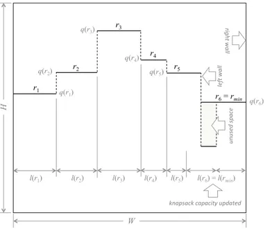
4.3 The skyline updated by adding the new roofs, renumbering, and enlarging r6to its left with the unused space (dashed area). After update, it turns out in this example rmin=r6. . . 57

4.4 Lmax obtained with the tightest packing of an EDD rank (left) and the tightest packing at all. . . 60

4.5 Aid= light grey area; A_¯X−Aid= dark grey area; ¯x= (¯zi, ¯ℓ_i₎, i₌ 1, . . . , p, are the solution values in the heuristic frontier ¯X. . . . 68

5.1 a) optimal for t = 0 and sub-optimal for t= 1; b) optimal for t=1 and sub-optimal for t=0 . . . 75

6.1 kω Ufor several γ values and ω(G)≤50 . . . 93

6.2 Star reformulation on a kite graph,|V| =5,|E| =6 . . . 95

6.3 Upper bound on|Q|values set by (6.36) . . . 98

6.4 min{OG[Cγ], OG[ ¯Cγ]}for different γ and graph densities . . . 102

6.5 Performance profile of gaps OGk_U and OG_¯k_U . . . 103 6.6 Performance profile of gaps OG_[DS

(18)

6.7 Performance profile of CPU running times for computing QU [DS

γ]

and QU

[Cγ]on sparse graphs. . . 105

6.8 Performance profile of gaps OG_[DS

γ] and OG[ ¯Cγ] on DIMACS

graphs. . . 106 6.9 Performance profile of CPU running times for computing QU

[DS

γ]

and QU

(19)

List of Tables

3.1 Results without precut on ten real instances. . . 40

3.2 Results with precut on ten real instances. . . 41

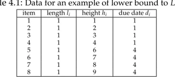
4.1 Data for an example of lower bound to Lmax. . . 59

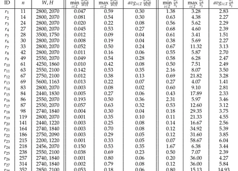
4.2 details ofIR-instances. The complete set of instances is available from the author. . . 62

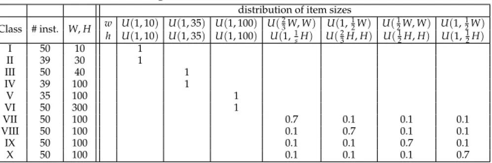
4.3 instances in I_B: bin size and assortment of item sizes for each class . . 63

4.4 SVC-DD, SVC2BPRF and best H solutions of 2BP on I_B: n mean values 63 4.5 MXGA_{and SVC-DD solutions of 2RBP-DD on I}_B_{: G}_N_{and G}_L_gaps₍_%₎ 65 4.6 MXGA, CPMIP and SVC-DD π_ℓsolutions of 2RBP-DD on I_B: G_Lgaps (%) . . . 66

4.7 SVC-DD∗ _{solutions of 2RBP-DD on I}_B_{: ¯R}₁_{, G}_A₍_%₎ _{and structure of} Pareto-frontiers. . . 68

4.8 SVC-DD∗ _{solutions of 2OBP-DD on I}_B_{: ¯R}₁_{, G}_A₍_%₎ _{and structure of} Pareto-frontiers. . . 69

4.9 SVC-DD∗solutions of 2RBP-DD on I_Rand due-date type C. . . 70

4.10 SVC-DD∗_{solutions of 2OBP-DD on I}_R_{and due-date type C.} . . . 71

5.1 Mean values of Ω%and ∆timegrouped by instance size n for α1=0.5.. 83

5.2 Integrality gaps with respect to the best primal solution. . . 84

6.1 percentage optimality gaps on random graphs . . . 110

6.2 Attributes of sparse graphs . . . 111

6.3 Attributes of DIMACS graphs . . . 111

6.4 percentage optimality gaps obtained with the dual bounds kU and ¯kU . . . 112

6.5 percentage optimality gaps obtained with the dual bounds kU and ¯kU . . . 113

6.6 percentage optimality gaps on sparse graphs . . . 114

6.7 CPU times on sparse graphs (in sec.) . . . 114

6.8 percentage optimality gaps on DIMACS graphs . . . 115

6.9 percentage optimality gaps on DIMACS graphs . . . 116

6.10 CPU times on DIMACS graphs (in sec.) . . . 117

(20)

(21)

Chapter 1 Introduction

The definition of many optimization problems is suggested and/or supported by the necessity of solving practical issues encountered in different fields, such as economic, biologic and social environments to be not exhaustive. A broad group of these problems can be ascribed to the family of the SET PACKING PROBLEM(SPP) in which, given a set of elements, the objective claims to max-imize (minmax-imize) a cost function associated to the assortments of subsets, so that a formal description of subset feasibility is fulfilled and the solution de-fines a packing of the elements. More specifically, the selection of subsets must be done in order to ensure an empty intersection between subsets so that each element is packed at most once. According to the computational complexity theory, the decision version of the SPP is a classical NP-complete problem and was included in the Karp’s 21 NP-complete problems [75]. Thus, the corre-sponding optimization problems are extremely challenging to be solved.

To give a practical application of SPP, one can refer to the CREW SCHEDUL-INGPROBLEMin airlines. In this problem crews must be assigned to airplanes in the fleet, so that flights can proceed in respect of the compiled timetables and the shifts of crew members meet the specifications of the labor contract. Crews are composed by staff members according to the skills and traits of the employers, such as the competence in piloting different types of aircrafts and the personal affinity with other crew members. Subsets of elements are built on all the possible crew and plane assignments, so that crew members and aircrafts are not shared among different concurrent flights. This corresponds to a packing of crews and planes.

Based on the statement of SPP one can give a general abstraction of prob-lems that emerge from very different environments, skimming from the de-tails that are applications-dependent. However, such dede-tails can be used to sketch an informal typology of SPP subfamilies by classifying the elements of the packing and interpreting the meaning behind the requirements of subsets. Among the wide family of SPPs, we focused on problems that are members of two subfamilies: the geometric packing problems and the structure packing problem. In the geometric packing elements are items characterized by

(22)

geo-metric sizes that must be inserted within larger objects of limited sizes. The feasibility of subsets is defined according to physical criteria that reflects the practical rules of a packing, such as the whole containment of items within boundaries or the non-overlapping between items. A noteworthy example of geometric packing is represented by the BINPACKINGPROBLEM(BPP) in which r-dimensional items must be placed into r-dimensional bins and the number of employed bins for the packing is minimized.

With structure packing we refer to the group of SPPs defined on graphs that ask for the search of graph substructures meeting packing constraints. The el-ements of the problem are generally represented by vertices and edges of the underlying graph, and the feasibility of subsets is established according to the fulfillment of requirements based (for instance) on measures of distance, den-sity and/or connectivity. An essential optimization problem of this category is the NODEPACKING PROBLEM, also known as VERTEX PACKING, MAXIMAL INDEPENDENT SET or STABLE SET problems [98]. Here we look for a max-imum subset of vertices such that, for each selected vertex, the set of edges incident on such vertex has an empty intersection with the sets of incident edges on all the other selected vertices; that is, each edge is incident on at most one of the selected vertices.

Our goal in this thesis is to study problems belonging to the SPP family and devise approaches to obtain primal and dual bounds for them. In particular, the methods implemented for SPP solution are the so called delayed column generationtechnique and sequential value correction heuristic, which make use of the concept of reduced costs (in a direct or indirect way) and are related to the solution of pricing subproblems. A formal introduction to these methods is given over the rest of the chapter, passing through notions of linear program-ming and integer reformulation.

1.1 Some preliminaries on linear programming

Mathematical programming can be intended as a general advanced language employed to describe optimization problems in a formal way. It is possible to classify problems by looking at the "shape" of a mathematical formulation and mathematical programming represents a valid solution methodology.

Before discussing the techniques employed in this thesis, we give some ba-sic elements about general linear programming problem [116]. The elements that compose a linear formulation are a vector of decision variables x∈R_nused to represent the decision in a problem, an objective function cT_x_{to be minimized} (maximized) where c ∈R_nis the cost vector, a set of constraints Ax ₌_bthat defines the feasible region expressed compactly, with the matrix of coefficient A∈ R_m_×nand the coefficient vector b _∈Rm. The set P₌ _{_x_∈ R_n_|_Ax₌_b_}

(23)

1.1 Some preliminaries on linear programming is called polyhedron.

Linear program (LP) are characterized by continuous variables, linear con-straints and objective function. When the decision variables are subjected to integrality, i.e. x∈Z, the result is an integer program (IP). Finally, if a formu-lation presents both continuous and integer variables, a mixed integer pro-gram (MIP) is addressed.

The linear programming problemPin standard form can be written as min cT_x

Ax = b

x ≥ 0.

A solution x∗ _∈ _P_{is optimal if it satisfies all the constraints and reaches the} global minimum of the objective function.

Given the primal LP problemP, the dual formulationDreads as max yT_b

yTA ≤ cT.

Independently on the chances that one has to find an optimum solution, the dual bounds that can be obtained via linear programming are very useful in practice and can provide a measure of the efficiency or effectiveness of the operational solution.

From the linear programming theory, a solution of P is optimal if all the reduced costsare non-negative, that is

cT−yTA≥0. (1.1)

Intuitively, the j-th reduced cost indicates the cost in terms of objective func-tion value to increase variable xjby a small amount, whereas the j-th compo-nent of the dual vector yjcan be interpreted as the marginal cost or shadow price to be paid for increasing bjby one unit. As you will see in the next sections, reduced costs have a crucial role in column generation procedure and inspired the sequential value correction heuristic framework.

We conclude this section by introducing an essential result from linear pro-gramming theory that is preparatory to the comprehension of the subsequent contents.

A solution vector x∈Pis an extreme point of P if it is not possible to express it as a convex combination of two other vectors v1, v2 ∈ P; that is, for any scalar α∈ [0, 1]there are no v1, v2∈ Psuch that x=αv1+ (1−α)v2. For any fixed vector v∈ P, the recession cone is defined as the set of all the directions

(24)

dthat start from v and move indefinitely away from it without leaving P, formally

{d∈R_n_|_Ad₌₀, d_≥₀_}.

Any non-zero vector of the recession cone is called ray and those rays that satisfy n−1 linear independent constraints to equality are defined as extreme rays. The extreme rays of the recession cone associated to a non-empty poly-hedron P are referred as the extreme rays of P.

The fundamental result of linear programming theory is the following Weyl-Minkowski theorem, also known as resolution theorem [116]:

Theorem 1. Let P a non-empty polyhedron with at least one extreme point. Given the set of extreme points v1, . . . , v|Q| _{and the set of extreme rays u}1_{, . . . , u}|R|_{of P,} then each point x∈P can be expressed as

x₌

∑

q_∈Q βqvq+

∑

r∈R γrur (1.2) with ∑q_∈Qβq=1, β∈R+_|Q|and γ∈R+_|R|.

Informally, theorem 1 states that each point of a polyhedron can be ex-pressed as a convex combination of the extreme points plus a non-negative combination of the extreme rays.

1.2 Dantzig-Wolfe decomposition

The Dantzig-Wolfe decomposition principle was firstly introduced in 1960 [45] in order to cope with large scale linear programming problems by extending the applicability of LP solution techniques. Indeed, the general idea behind decomposition is to exploit the structure of the problem to reformulate it in an equivalent fashion, which is however convenient under certain points of views (e.g. quality of linear relaxation, computational burden in solution). The effectiveness of such technique was largely assessed throughout the years since its first application by Gilmore and Gomory [62, 63]. Thus, the decom-position approach became a standard methodology to whom several papers and book chapters are dedicated [99, 118].

Let us consider the following LP, usually called compact formulation (L):

min cT_x _(1.3)

Ax ≥ b (1.4)

Dx ≥ d (1.5)

(25)

1.2 Dantzig-Wolfe decomposition Let moreover assume that the polyhedron P = {x ∈ R+_n_|_Dx _≥ _d_}is non-empty. By theorem 1, we can substitute x∈ Pand rewrite formulationLin the equivalent extensive formulation (RL):

min

∑

q∈Q ¯cqβq+

∑

r∈R ¯crγr (1.7)

∑

q∈Q ¯aqβq+

∑

r∈R ¯arγr ≥ b (1.8)

∑

q∈Q βq = 1 (1.9) β _∈ R+ |Q| (1.10) γ _∈ R+ |R| (1.11)

where ¯cq=cTvqand ¯aq=Avqfor q∈Q, ¯cr =cTur and ¯ar =Aurfor r∈R. Formulation RL has a reduced number of constraints with respect toLas (1.5) disappeared and only the convexity constraint (1.9) is added. Neverthe-less, the number of variables may become exponential due to the number of extreme points (rays) and solvingRL can be impractical. Hence, a column generation procedure is usually employed to solveRL by considering only a subset of columns, while missing columns are generated on the fly when needed. Details about column generation algorithm are given later, we now focus on the integer akin to the decomposition for IPs.

1.2.1 Decomposition of IP

Let us introduce the following IP (I):

min cT_x _(1.12)

Ax ≥ b (1.13)

x ∈ X (1.14)

where X=P∩Z+and P is defined as above.

When reformulating an IP or an MIP, decomposition can be performed ac-cordingly to two main techniques: convexification or discretization [83]. The convexification is based on replacing X with its convex hull (conv(X)) and ex-pressing x in terms of the extreme points and extreme rays of conv(X). How-ever, after applying convexification the integrality constraints on original vari-ables are still required and such varivari-ables cannot be put aside. Indeed, it is insufficient to enforce integrality on variables β and γ to obtain an equivalent representation ofI, as its optimal integer solution could be an interior point of conv(X). Nevertheless, a remarkable exception is given for X⊆ [0, 1]n_since

(26)

all its integer points are vertices of conv(X). Generally speaking, to obtain a true integer equivalent ofIone must rely on discretization, which is based on the extension of theorem 1 for the integer case [99]:

Theorem 2. Let P a non-empty polyhedron and X= P∩Z+_{. Then, there exists a} finite set of integer points v1, . . . , v|Q| ⊆X and the set of integer rays u1, . . . , u|R|⊆

P such that each point x∈X can be expressed as x₌

_∑

q∈Q βqvq+

∑

r∈R γrur (1.15) with ∑q∈Qβq=1, β∈Z+_|Q|and γ ∈Z+_|R|.

Theorem 2 allows to express each point of a polyhedron as a convex combi-nation of integer points plus a non negative combicombi-nation of integer rays. We can then reformulateI in the equivalent extensive formulation (RI):

min

∑

q∈Q ¯cqβq+

∑

r∈R ¯crγr (1.16)

∑

q∈Q ¯aqβq+

∑

r∈R ¯arγr ≥ b (1.17)

∑

q∈Q βq = 1 (1.18) β _∈ Z+ |Q| (1.19) γ _∈ Z+ |R| (1.20)

where ¯cq=cTvqand ¯aq=Avqfor q∈Q, ¯cr =cTur and ¯ar =Aurfor r∈R.

1.2.2 The case of block-angular structure

It frequently happens that problems present a matrix coefficient D with a mod-ular structure that can be exploited when applying decomposition techniques. Let K be the set of independent blocks in which D can be partitioned. Figure 1.1 gives an insight of the block-angular structure.

We can identify|K|disjointed polyhedra Pk ₌_{_xk _∈_R+

nk|Dkxk ≥d

k

}such that Xk₌_Pk_∩_Z+_{. Then,}_I_{can be rewritten in}

min

∑

k∈K (ck)Txk (1.21)

∑

k∈K Akxk ≥ b (1.22) xk ∈ Xk ∀k∈K. (1.23)

(27)

(28)

common to refer to CG with the acceptation of delayed to highlight the pecu-liarity of the scheme, which implicitly enumerates the columns in place of a full a priori description of them in the formulation.

Given an LP formulation restricted to a subset of columns, namely re-stricted master problem, a CG algorithm performs a search of columns (vari-ables) among the ones that are not explicitly included. The search looks for non-basic variables to be added that have reduced costs able to possibly im-prove the objective function value. This functioning reflects the selection of pivot elements in the simplex method and lay the groundwork on the linear programming theory. Typically, the search of profitable columns is performed by relying on a pricing subproblem that is fed with the values of dual variables taken from the current optimal solution of the restricted master problem. The solutions of the pricing subproblem are used to generate the missing columns, which are added to the restricted master problem. The dual variables are then updated by solving the restricted master problem and the whole loop is iter-ated, until the global optimality of the restricted master problem is certified by fulfilling condition (1.1).

To formalize, let us indicateRI as master problem. Moreover, let us call ˜RI the restricted master problem obtained by relaxing the integrality constraints in formulationRI, while restricting variables βk and γk taken into account to the subsets of integer points ˜Qk ⊆ Qk and integer rays ˜Rk ⊆ Rk for each k∈ K. Finally, let us refer to the dual variables of constraints (1.25) and (1.26) as θ and ψ, respectively.

The reduced cost of a column inRI for a fixed k∈Kis generally expressed as

h

(ck)T−θAkivkq−ψk ∀q∈Qk h

(ck)T−θAkiukr ∀r∈Rk

for integer points q and integer rays r. Given a dual optimal solution (θ∗_{, ψ}∗₎ of ˜RI, the k-th pricing problem Pr(k)called to find the most profitable column for block k is:

Ωk=minh(ck)T₋_θ∗_Aki_p ₋ _ψ∗ _(1.29)

Dkp ≥ dk (1.30)

p ∈ Z+

nk. (1.31)

For Ωk _<_{0 and finite, the optimal solution vector p}_∗_{is an integer point v}k qto be added to ˜Qk. The corresponding column βk_{q, with coefficients}h_¯ck_{q, ¯a}k_{q, 1}iT_, is generated and added to ˜RI. When Pr(k)is unbounded, p∗ represents an

(29)

1.4 Sequential value correction heuristic integer ray uk

qto append into ˜Rk. In this case, the column γkqis generated with coefficienth¯ck

q, ¯akq, 0 iT

and ˜RI is properly updated. Finally, if Ωk≥0 for each k∈ K, then all reduced costs are non-negative and condition (1.1) is satisfied, so that ˜RI is solved to optimality. Clearly, the optimal value of ˜RI is a valid lower bound forRI.

Pr(k)is an IP that can be challenging to solve, thus the performance of the whole CG procedure can be compromised. To accelerate the convergence of the algorithm, one can rely on efficient heuristics or combinatorial algorithms to generate profitable columns, even more than one concurrently for each pric-ing subproblem. However, (1.1) need to be certified by solvpric-ing Pr(k)exactly for all k∈K.

Unfortunately, it happens quite often that the convergence of the CG proce-dure requires several iterations, since the values of the dual variables follow an oscillatory dynamic [51] and the optimal solution of ˜RI can be degenerate. The phenomenon of the slow convergence is generally indicated as tailing-off effect. To overcome this issue and improve the CG performance, several stabilization techniques have been developed, e.g. the box step method [90], bundle methods [69] and primal-dual stabilization strategies [94, 21].

The CG procedure can be embedded in the branch-and-bound framework to find optimal integer solutions ofRI, resulting in the so called branch-and-pricescheme [15, 128]. Alternatively, algorithms based on CG and designed ad hoc for integer programming problems have been presented in literature. Ap-plications of integer programming CG can be found for the VEHICLE ROUT-INGPROBLEM [48], the CREW SCHEDULING PROBLEM[50], the TRAVELING SALESMANPROBLEM[49], the STABLESETPROBLEM[28] to mention a few. A useful list of these applications is reported in [83].

1.4 Sequential value correction heuristic

The sequential value correction heuristic (SVC) is a successful technique largely employed to obtain good primal solutions for BPP and CSP in limited amount of time. Firstly introduced in Mukhachiova and Zalgaller [96], the SVC be-longs to the family of sequential heuristics for BPP and CUTTING STOCK PROBLEM (CSP) that construct one pattern per time accordingly to a cus-tomized strategy [65, 139, 126, 77]. Indeed, it can be classified as an iterative greedy method in which the space of search is probed following the trajectory described by the dynamic of the so-called pseudo-prices. Recall that in the one-dimensional CSP, which generalizes the NP-hard bin packing problem [61], a set of small items I with length li have to be cut from large stock items of size l, so that the corresponding demand riis fulfilled and the total

(30)

produc-Figure 1.2: SVC flow chart

tion waste is minimized. A more precise formalization of this combinatorial optimization problem will be given in §2, we here contextualize to introduce the basic notation.

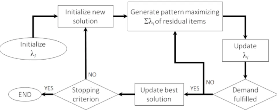
In the SVC framework (see figure 1.2), a pseudo-price λi is defined as a value associated to each item i∈ I. After the initialization, a pattern is built by solving an appropriate pricing subproblem in which items are inserted in order to maximize the total sum of the selected item pseudo-prices. Such functioning clearly recall a similarity between the pseudo-prices and the role of the shadow prices in the CG procedure, that guide the generation of new profitable patterns (by which the name pseudo-price derives). Once no more items can be inserted in a pattern, an updating phase modifies the values of the pseudo-prices by perturbing them according to formulae that generally take into account the quality of the last computed pattern. Then, the level of activation of the pattern is decided and if the demand is not completely fulfilled, a new pattern is generated by iterating the process. Otherwise, the solution found is evaluated and it is recorded as best incumbent if improv-ing the objective function. The algorithm ends if the stoppimprov-ing criteria (e.g., time limit, number of iterations or lower bounds) are met, or alternatively the whole process is repeated starting from the initialization of a new empty so-lution. Typically, solutions found by the SVC algorithm describe a dynamic of the objective function values characterized by a rapid decrease in the first iter-ations, followed by fluctuations nearby the optimal value for the subsequent ones.

The general description of the SVC heuristic was translated into different implementation across the years and the main differences usually emerge in the initialization and updating phases of the λiterms. The definitions of both steps can be specified in a wide spectrum of possibilities that generally reflect the features of the application and are customized on the specific problem to achieve high performances.

(31)

1.4 Sequential value correction heuristic The first application of SVC was presented by Mukhacheva and Zalgaller [96], who proposed it in the contexts (among others) of cutting forming prob-lems and probprob-lems of cutting totality planning with intensities of their ap-plication. For the sake of exemplification, some details of their deterministic implementation are reported. The exploited formulae are based on the mea-sure of trim losses ωp_{of pattern p}_∈_P_{and material consumption of each item} i ∈ I. Let λ0

i be the starting value of the pseudo-price of item i and λhi the corresponding value after the computation of the h-th pattern. Given a CSP solution computed by means of first-fit decreasing (FFD) algorithm with NFDD patterns, the authors initialize the pseudo-prices as

λ0_i = lil ri NFDD

∑

p=1 ap_i l−ωp i∈ I (1.32)

where a_ipgives the number of parts i produced in pattern p ∈ P. Intuitively, for each pattern its trim loss is distributed across the width of the part-types that belong to it, in a way that is proportional to the number of times each item occurs.

After that a pattern p is completed by maximizing the total values of se-lected items, the pseudo-prices used for the following p+1-th pattern are set by λ_ip+1=λ_ip(1−a p i ri) + a_ip ri lil l−ωp i∈I (1.33)

in which the formula defines each new pseudo-price value to be the weighted sum of its previous value and the material consumption norm within the last obtained pattern.

Some years later the SVC scheme was employed again by Mukhacheva et al. [97] in one-dimensional CSP, and by Verkhoturov and Sergeyeva [131] for the two-dimensional CSP with irregular shapes. The latter dealt the issue of the item placement by defining the pseudo-prices as functions of the angle of rotation and such angles are chosen in order to maximize the pseudo-price values. Still, the formulae are deterministic, whereas in the former [97] the method was randomized to diversify the search and prevent cycling. Indeed, the pseudo-price formulation was modified by introducing the random pa-rameter ξ as λp+1_i = λ p iξ(bi+ri) ξ(bi+ri) +ap_i + a_ip ξ(bi+ri) +a_ip lil l−ωp i∈ I (1.34)

(32)

where biis the current residual demand of part-type i. The randomized SVC was embedded in a modified branch-and-bound scheme and, even if it re-quired the tuning of bounds for parameter ξ, (1.34) proved its effectiveness by improving the performance with respect to the deterministic counterpart (1.33).

Relevant subsequent implementations of the SVC can be found in Belov and Scheithauer [18], where the heuristic was embedded in a cutting plane algorithm to solve the one-dimensional CSP with multiple stock widths and the pseudo-prices are initialized with the value of the dual variables of the LP relaxation solution; in [17] by the same authors, in which the SVC is called to solve the residual problem that arises after rounding the LP solutions within a branch-and-cut-and-price scheme. This algorithm is based on strengthening the LP relaxation of branch-and-price nodes by applying Chvátal-Gomory and Gomory mixed-integer cuts [100]. It was applied both to one-dimensional and two-dimensional two-stage guillotine constrained CSP.

In [19] the pseudo-prices updating phase is modified in order to balance the distribution of large items across the sequence of generated patterns. In-deed, the concentration of small items generally gives patterns with a high total price and low trim-loss, that however limits the possibilities to get good patterns with the remaining large items. Inspired by the max-len-mini-items heuristic of Kupke [77] that limits the number of items in each pattern, the SVC was thus changed by using pseudo-prices over-proportional to the item widths, so that prices of large items are supported and patterns with mixed combinations of widths are favored. The SVC heuristic in [19] is moreover customized to deal with the multi-objective CSP, in which the minimization of setups and open-stacks is asked along with the reduction of trim-loss. In particular, when the attention is focused on the open-stacks minimization, the pseudo-prices of all items with open order are multiplied by an exponential factor, thus reducing the chance of opening new stacks.

Further employments of the SVC heuristic were presented for the two-dimensional strip-packing problem by Belov at al. [20] and Cui et al. [40] respectively for the orthogonal and non-oriented case, where the latter took into account both the presence and absence of guillotine constraints. More recently, Cui et al. [41] inherited the value correction principle for a sequen-tial pattern-set generation algorithm designed to solve one-dimensional CSP with setup costs. In [33] Chen et al. exploited the SVC scheme to compute both guillotine and non-guillotine patterns for the two-dimensional BPP. Arbib and Marinelli [12] dealt with the minimization of a convex combination of num-ber of bins and maximum lateness in a one-dimensional BPP integrated with scheduling features, in which orders must be fulfilled within prescribed due-dates. The proposed price-and-branch uses primal solutions built by means

(33)

1.5 Chapter Outline of an SVC algorithm. Finally, in [34] a CSP with skiving option which derives from paper and plastic film industries is investigated and an SVC heuristic is combined with two integer programming formulations to solve two specifica-tions of the problem.

1.5 Chapter Outline

The rest of the thesis is structured as follows:

• In chapter 2 we focus the discussion on selected geometric packing prob-lems derived from real manufacturing scenarios that are characterized by scheduling aspects. Looking at the representative mathematical pro-gramming formulations for these problems, the aim is to provide a use-ful insight to integrate two perspectives, the packing and the scheduling ones, under a unifying framework.

• Chapter 3 is devoted to a multi-stock CSP arising in woodboard man-ufacturing systems, in which real aspects are taken into account along with multiple objectives. An SVC algorithm is described in detail, which was designed with the aim of identifying sets of non-dominated solu-tions. The quality of solutions is discussed by comparison with a bench-mark software exploited in a real manufacturing system.

• In chapter 4 we discuss a bi-objective extension of BPP in which items are provided with due-dates and the maximum lateness in the packing process has to be minimized along with the number of employed bins. The problem is coped by means of an SVC heuristic, while bi-objective approximation results are derived from BPP heuristics with guaranteed approximation ratio.

• Chapter 5 deals with a BPP with due-dates that embeds the presence of items processing time in the packing operations. In this context the completion time of a bin is dependent by the multiplicity of the items packed within and the objective is formalized as a convex combination of the number of used bins and the maximum lateness across the pro-cess. An integer pattern-based reformulation solved by CG is presented for this problem and evaluated with respect to an assignment compact formulation in terms of continuous bound quality.

• Chapter 6 is related to a structure packing problem called MAXIMUM QUASI-CLIQUE PROBLEM (γ-QCP). Indeed, the clique is a cohesive structure complementary to the independent set that can be seen under

(34)

the viewpoint of a packing problem. The γ-QCP is a combinatorial op-timization problem in which a γ-quasi-clique, that is a clique relaxed on the density constraint, is sought while maximizing the order of the set of selected vertices. We present an original integer reformulation with surrogate relaxation to achieve dual bounds by means of CG procedure. Moreover, the connectivity issue for subgraph structures is discussed and a new sufficient condition on solution connectivity is presented and computationally evaluated.

• Finally, chapter 7 is devoted to the concluding remarks of the thesis and to give some potential directions for future research.

(35)

Chapter 2 Cutting processes optimization

The majority of the results presented in this thesis were achieved in the field of bin packing and cutting problems, generally enriched with constraints and features that emerge from real manufacturing scenarios and are closely related to the scheduling of operations. In order to portray the connection that exists in the real environments between packing (cutting) and scheduling aspects, this second chapter want to be a non-exhaustive tentative to integrate the two perspectives under a unifying framework, focusing on representative mathe-matical programming models.

2.1 Introduction

In general terms, a common feature of packing problems is that they deal with bounded geometric figures (r-dimensional compact sets) that are not de-formable, cannot overlap, and must be placed into larger geometric figures, either bounded or unbounded. Due to a mathematical affinity to cutting prob-lems, where figures are components (here called small items) to be cut from big plates (large items), these problems are gathered into the larger family of cutting and packingproblems (C&P), including such well known basic models as KNAPSACK, PALLET LOADING, BPP. Among others, the CSP is one of the best known C&P problems in both the practitioner community – for its prac-tical relevance – and the research one – due to the mathemaprac-tical properties exploited for its solution. Although C&P problems usually emerge in manu-facturing environments, related applications include issues derived from dif-ferent contexts, such as the data packets allocation in telecommunication field [82]. Moreover, BPP and CSP can be seen as special cases of the VEHICLE ROUTINGPROBLEM[49].

The basic CSP calls for fulfilling a given demand of small items of various sizes, and possibly shapes, by cutting standard large items of identical size, with the objective of minimizing the amount of unused material. It has almost uncountable variants and extensions that depend on geometrical features, | the dimension of the things to cut (one, two or three), their shape (rectangles,

(36)

spheres, general convex or non-convex figures), etc. | on the technique used to obtain the shapes, | simple or nested cuts, guillotine cuts in one or more stages, fretwork, part rotation, leftovers reuse allowed or not etc. | on the as-sortment of either small or large items, | of either small (one, few of many part sizes) or large items (one, many identical, distinct or unbounded stock plates) | and on the type of assignment of small to large items. For a comprehensive typology, see [135]. Whatever is the variant considered, a solution of the CSP is in general a non-ordered set of cutting patterns, each one associated with a positive integer called activation level or run length. A cutting pattern specifies the small items and their geometrical arrangement that must be cut from each large item, and its run length is the number of large items to be cut in that way. Now, cutting machines generally implement the same cutting pattern on a single, limited pack of large items at a time and each single cut, as well as the total process, can be organized in many ways that affect system performance. Crucial elements for a correct management of a cutting process are:

• The way each machine implements a cutting pattern: for instance, mul-tiple parallel cut vs single sequential cut: a sequential cutter (e.g., a pan-tograph milling machine for irregular shapes) implements each pattern by cutting the small items in a sequence, and different sequences may take different time.

• The number, type and duration of set-ups, given by slitter repositioning or other types of changeover; set-ups may occur from pattern to pattern, so that solutions with few different patterns can be preferred to ones with many; furthermore, switching time may depend on consecutive pattern pairs.

• The organization of demanded production (and therefore of the patterns it derives from) as desired by downstream plant departments: for exam-ple, lots can be required in prescribed sequences or within given due-dates; similarly, large items of different sizes can be subject to different release dates.

• The finite capacity of the buffers designed to accommodate the small items, and so to divide the production by classes (e.g., by order or shape): in this case not all patterns and not all pattern sequences are feasible, because they may produce an excess of some part class. Summarizing, patterns and run lengths normally give insufficient informa-tion to implement a soluinforma-tion, and a subsequent effort to organize the process is normally required to schedule cuts after a CSP solution has been found (cut-then-schedule). However, not only is this approach generally sub-optimal, but also traditional CSP objectives may drive patterns and run lengths towards

(37)

2.1 Introduction poor or even infeasible choices. With a simultaneous approach that takes those issues into account (cut-and-schedule), CSP models are enriched in or-der to define quality and feasibility of the schedules in which pattern and/or cuts within patterns are organized. In such models, a solution is what we here call a cutting plan.

The above discussion suggests that, in industrial applications, the problem of finding an optimal cutting plan combines so many varieties that it is dif-ficult to get a comprehensive picture. Thus, we prefer to focus here on few issues that are common to a large amount of manufacturing environments:(i)

reduction of the number of set-ups,(ii)minimization of delays in the delivery of the parts required, and(iii)scheduling of cut-operations when intermedi-ate stacks have a finite capacity. This focus has the advantage of illustrating three different fundamental ways of considering process efficiency without getting lost in implementation details not always worth of consideration from a scientific viewpoint.

Issue(i)deals with machine productivity and is traditionally considered a very important cost source in manufacturing. It originates the so called PAT -TERNMINIMIZATIONPROBLEM(PMP), in which the number of set-ups, that incur at slitter repositioning, has to be minimized.

Issue(ii)arises when material cutting not only has a local dimension of pro-cess efficiency, but also one related to customer satisfaction, or to the synchro-nization with other processes. In the corresponding CSP extension (CSP-DD), lots are provided with individual due-dates and the goal, jointly with material usage optimization, is the minimization of due-date related scheduling func-tions: typical objectives are the minimization of maximum or weighted tardiness, or of the number of tardy jobs.

Issue (iii) emerges because industrial production is often organized in lots, that can be either homogeneous (namely, formed by parts of the same size/type), or heterogeneous (for instance when different part types are grouped to form a particular client order). Real cutting processes often try to limit the variety of unfinished lots simultaneously present in the system. This translates into a problem called STACK-CONSTRAINEDCSP (SC-CSP), where feasible plans are allowed to maintain a maximum number of open stacks at any time (a stack is regarded as open as far as it is occupied by an uncom-pleted lot). Minimizing the number of open stacks is recommended in order to reduce the possibility of errors as well as in-process inventory [11], and in some cases (e.g., wood-cutting) it derives from the very technical require-ments of machines.

In this chapter we discuss representative models in which optimal/feasible cutting plans are so defined as to cope with the aforementioned CSP exten-sions. Specifically, after a brief historical excursus that focuses on the main

(38)

achievements obtained to deal with CSP, we formally define in §2.2 the prob-lem of identifying an optimal cutting plan; then, mixed integer linear pro-gramming (MILP) formulations will be respectively reviewed, under a unify-ing notation, for three representative CSP extensions: PMP in §2.3, CSP-DD in §2.4 and SC-CSP in §2.5. Note that the exposition focuses on the cut-and-scheduleperspective and the dissertation could be refined by including also the cut-then-schedule counterpart. However, this has been considered beyond the purpose of the chapter.

2.1.1 An historical overview

In 1960, the one-dimensional version of the problem, that is, cutting shorter bars of various given length from longer bars of standard length available from stock, received by Kantorovich [74] a first formalization in terms of an integer linear programming model. This model makes use of assignment vari-ables uijthat count how many parts of lot i∈ Iare produced by stock bar j∈J. An extra 0-1 variable wjfor each j∈ Jtells whether that bar is actually cut or not and, summed up for all the stock bars available, all these extra variables give the amount of material used to cut the required parts.

The assignment integer linear programming formulation report as follows:

min

∑

j_∈J wj (2.1)

∑

j_∈J uij = ri i∈I (2.2)

∑

i_∈I liuij ≤ lwj j∈ J (2.3) uij ∈ Z+ _i_∈I, j_∈ _J (2.4) wj ∈ {0, 1} j∈ J. (2.5)

The objective function (2.1) is defined as the minimization of the total num-ber of employed stock bar, under the satisfaction of constraints (2.2) that im-poses the required number of parts ri to be cut for each part-types i ∈ I. Fi-nally, the limited length l of the stock bars obliges variables to obey integer knapsack constraints (2.3).

This model has severe limitations, not only due to the potentially large num-ber of variables (pseudo-polynomial with the numnum-ber of part types), but also, most of all, to the poor quality of the lower bound obtained by linear relax-ation and the strong symmetry shown by feasible solutions. Such issues can be related to the excessive finesse of the grain used to describe solutions, that is actually relevant only when some additional practical aspects are integrated

(39)

2.1 Introduction to the basic CSP definition.

One year later, Gilmore and Gomory [62] published a key reformulation of Kantorovich’s model, based on Dantzig-Wolfe decomposition. Let aip be the number of parts of lot i∈ Iproduced with one stock item cut according to pattern p ∈ P, where P is the set of enumerated patterns. By using the integer variables xp_{to count the activation level of pattern p}_∈ _{P, the integer} reformulation results in:

min

∑

p∈P xp (2.6)

∑

p_∈P a_ipxp = ri i∈ I (2.7) xp ∈ N _p_∈P. (2.8)

By replacing the knapsack constraints (2.3) by the convex hull of their inte-ger solutions, the new pattern-based model drastically improved the LP lower bound and eliminated solution symmetries. Also, it opened a way to investi-gate on the so called integer round-up property (IRUP, [16]), that occurs when the integer optimum z∗_{equals the LP lower bound, i.e., the smallest integer} greater than or equal to the optimum value of the LP relaxation (see [86, 85] for details).

Nevertheless, the formulation of Gilmore-Gomory has an exponential num-ber of variables due to the numnum-ber of different combinations in which a stock item can be cut. Hence, solving its linear relaxation requires the call to a de-layed column generation technique, which relies on the solution of a pricing problem to generate profitable columns. In the one-dimensional case, such pricing is modeled as an integer knapsack in which the a_ip’s appear as deci-sion variables piand are generated from the pricing solutions.

Finding exactly optimal integer solutions remained a challenge for several years, as the column generation allows computing only the LP optimal value. On the other hand, some heuristic approaches performed very well due to the structural properties of rounding, especially for high-demand instances [119, 134].

A breakthrough was represented by the seminal work of Barnhardt et al. [15] in 1996 that introduced the branch-and-price technique and allowed the solution of one-dimensional CSP instances with hundreds of items [6].

Nowadays, the available approaches make possible to solve pure CSP in-stances with size that widely exceed the requirements of real production sys-tems. Thus, the attention of the research community move forward, focusing on a wider perspective in which the technological and managerial issues of cutting processes are taken into account. This is also merit of a spreading

(40)

sen-sibility that recognizes the solutions of pure CSP as hardly or even impossible to be implemented in practice, given the presence of productive constraints and the impact of significant scheduling-related objectives [73].

2.2 General problem definition

In general terms, the problem of finding a cutting plan can be stated in this way:

Problem 2.2.1. Find a set of patterns, their run lengths and implementation (pattern assignment to machines and/or time instants) such that:

• the demand of all part types is fulfilled;

• the output schedule of lots is feasible and meets the desired level of performance; • the total trim-loss is minimized.

For ease of presentation we will regard lots as homogeneous, and assume that parts are cut from identical stock items. Formulations that generalize to heterogeneous lots and/or stock sizes can however be obtained straightfor-wardly.

The following list summarizes the notation used throughout the rest of the chapter.

Data:

I: set of lots (jobs),|I| =n;

P: set of patterns (implicitly enumerated),|P| =N;

li: length of the parts belonging to lot i∈ I(if one-dimensional); l: stock items length (if one-dimensional);

ri: volume (number of parts) of lot i∈ I; di: due-date of lot i∈ I;

T: index set of time periods dividing a given planning horizon;

a_ip: number of parts of lot i∈ Iproduced with one stock item cut according to pattern p∈ P.

A bar over a symbol makes it binary, giving 1 if>0 and 0 if_≤0. For instance,

¯ap

i means 1 if pattern p produces one or more parts of type i, and 0 otherwise. Note that the set T of time periods can be a decision variable, as a priori sub-divisions can have two types of drawbacks: high computational complexity if

(41)

2.2 General problem definition too fine-grained, bad approximation if too coarse-grained. Moreover, the time horizon can be divided in periods of non-equal lengths, and these lengths may not be known in advance.

Decision variables:

Ci ∈R+: completion time of lot i∈ I;

Ti ∈R+: tardiness of lot i: Ti₌max_{_Ci₋_di, 0_}, i_∈ I; Lmax ∈R+: maximum lateness of any lot: Lmax₌maxi_∈I_{_T_i_};

x_tp ∈ Z+: number of stock items cut in period t _∈ _Taccording to pattern p∈P(run length of pattern p in period t);

sit ∈Z+: inventory level (number of parts produced and not yet sent out) of lot i∈Iat the end of period t∈T;

θmax ∈ Z+: maximum number of lots simultaneously in process throughout the planning horizon;

yit ∈ {0, 1}: gets 1 if and only if lot i∈ Iis still in process in period t∈T; Again, we remove indexes in case of independence, and use a bar to “bina-rize” variables. In particular:

¯x_tp gets 1 if and only if pattern p is active in period t;

¯sit gets 1 if and only if one or more parts of type i are still in process during period t

¯Ti ∈ {0, 1}is used to count the number of tardy jobs.

Let x, σ denote vectors collecting variables x_tpand the remaining variables (sit, yit, etc.), respectively. The following formulationG updates Gilmore and Gomory’s model in order to give our problem a general framework:

min α1material-cost(x) +α2implementation-cost(x, σ) (2.9) subject to:

∑

p∈P a_ip

∑

t∈T xp_t = ri j∈J (2.10) (x, σ) ∈ R. (2.11)

The objective function (2.9) describes the convex combination of the two cost items, where α1, α2∈R+with α1+α2=1. Equality (2.10), sometimes re-laxed by≥or by constraining the left-hand side within a prescribed interval, is

(42)

the demand constraint. Clause (2.11) is a generic form for the implementation (e.g., scheduling) constraints, and regionRvaries according to application. For identical stock sizes, the first term of (2.9) has the form

τ=material-cost(x) =

∑

p∈P

∑

t∈T

x_tp (2.12)

and, if (2.10) is not relaxed, measures trim-loss.

When inventory levels are relevant, the demand constraint is replaced by equilibrium equations

si_,t−1+

∑

p∈P

a_ipx_tp=rit+sit i∈I, t∈T (2.13)

that involve inventory variables sit. The first term of the left-hand side and the last of the right-hand side give the amount of parts inherited at the beginning and left at the end of the period. By considering the set T of time periods partitioned into consecutive intervals[0, d1],[d1, d2], . . . ,[dn−1, dn],[dn, dn+1], where it is w.l.o.g. assumed 0< _d₁ _≤ _d₂ _≤ _{. . .}_≤ _dn _≤ _d_n+1_{, and dn+1}_{is the}

horizon length; then rit, the amount of parts of type i due by dt, is rifor i= t and 0 otherwise.

The above formulation is actually depicted for single machine CSP, in which patterns are sequentially implemented by the same machine. Nevertheless, real cutting processes are commonly carried out by more complex produc-tion systems with a structured layout. For instance, cutting operaproduc-tions can be split into two stages if an upstream machine divides each stock item into mparts, and each part is subsequently sent to one of m downstream parallel cutting machines. Another example is given by in-house precut, a practice especially operated by big plants that separately prepare stock material for warehouse, which will be used in consecutive processes. Looking at real cut-ting systems, the definition of optimal cutcut-ting plan gains features typical of scheduling problems with multiple machines. Specifically, a CSP is related to a parallel machine scheduling environment when machines separately and simultaneously operate for job fulfillment on independent job portions, and to a flow-shop environment when the cutting plan comprises a stream of op-erations performed by subsequent cutting machines. Although we here focus on single machine CSP, formulationGcan easily be adapted to multi-machine environments by suitably changing the definition of (some of) its components.

(43)

2.3 Set-up minimization

The problem of finding, among all the CSP optimal solutions, one that mini-mizes the number of patterns used and thus, for identical patterns, the set-ups required, was first considered by Vanderbeck [127] and called the PATTERN MINIMIZATIONPROBLEM(PMP).

Referring to the general model of §2.2, the problem has overweight material-cost(x) in objective (2.9), thence prioritizing trim-loss minimization. Integer variables xp_{expressing pattern run lengths need to be coupled with 0-1} pat-tern activation variables ¯xp_{, that summed up on P give the total number of} patterns used: min

∑

p∈P ¯xp _(2.14)

∑

p∈P xp ≤ τ∗ xp ≤ Up¯xp p∈P xp ∈ N, ¯xp _{∈ {}0, 1_} _p_∈_P

plus demand constraints (2.10) written for single period. In (2.14), τ∗_indicates the maximum admissible material usage, and the activation constraints uses adequate upper bounds Upon pattern run lengths.

In alternative, Vanderbeck [127] suggests one binary activation variable per pattern and per run length; that is, zxp=1 if and only if pattern p is activated at run length x: min

∑

p∈P Up

∑

x=1 zxp (2.15)

∑

p∈P Up

∑

x=1 xzxp ≤ τ∗ (2.16) zxp ∈ {0, 1} p∈P, x=1, . . . , Up subject to demand constraints

∑

p∈P Up

∑

x=1 xap_izxp = ri j∈ J. (2.17)

Both (2.14)+(2.10) and (2.15)-(2.17) can be derived by discretizing different subsets of constraints in a bilinear model, based on Kantorovich and enriched with pattern activation variables, see [5].

(44)

non-decreasing and super-additive, then also ∑j f(ai)xi ≤ f(b)is valid forP: rank 1 Chvátal-Gomory cuts are for instance derived using f(y) = ⌈λy⌉for 0<_λ<_{1. Cuts to strengthen Vanderbeck’s formulation can be derived with}

this technique from inequalities (2.16) and (2.17). In [127], the super-additive functions have the form fp(y) =⌈τpy∗⌉ −1 for (2.16) and fp(y) =⌈

pya_ip

ri ⌉ −1 for

(2.17). The derived cuts dominate Chvátal-Gomory’s, can be added without destroying the problem structure, and are separated in pseudo-polynomial time. Alves and Valério de Carvalho [6] propose dual feasible functions (DFF) that dominate the function proposed by Vanderbeck and, consequently, pro-vide sharper cuts. A DFF is a function f :[0, 1]→ [0, 1]such that

∑

µ∈H

µ≤1⇒

∑

µ∈H

f(µ)≤1

for any finite set H of real numbers. Let 0≤ai≤bwith b>0, and let primal xfulfil ∑_i=1n aixi≤b, i.e., ∑ni=1abixi ≤1. Rewrite the inequality as

n

∑

i=1 xi

∑

k=1 ai b ≤1. Sinceai

b ≤1, by definition of DFF we can replace it by f( ai

b)and stay feasible: therefore n

∑

i=1 xi

∑

k=1 f(ai b) = n

∑

i=1 f(ai b)xi≤1 is valid.

Comparison were performed on instances with up to 350 items to evaluate the LP relaxations of the two formulations and to point out the role played by the choice of upper bounds Up [5, 19]. In particular, the LP relaxation of (2.14)+(2.10) is showed to be theoretically tighter, although computational results give only evidence to a limited advantage.

A particular case of PMP, typical of situations with a fixed number of slit-ters, occurs when a cutting pattern can never produce more than a prescribed number u of small items. For u=2, the feasible patterns are in one-to-one cor-respondence with the edges of a compatibility graph G= (I, E), where(i, j)∈E means that a part of type i and one of type j can be cut from the same stock item.

McDiarmid [93] studied the special case of G=Kn, where any two parts fit any stock length, but no three do. In this problem, a crucial role is played by cut schedules. Since every pattern produces two parts, one can regard these two streams of parts as if they were produced by two parallel machines. A non-preemptive strategy is to produce the generic part type i continuously, as soon as the relevant lot is completed. Thus, the CSP is trivial, whereas the PMP

(45)

2.4 The CSP with due-dates (corresponding to maximizing the number of times two jobs end at the same time) is proved to be NP-hard [93]. The last observation leads to formulate the PMP in terms of SETPACKING, see [4].

A natural generalization of this problem describes the set of feasible pat-terns as the edge set of an undirected graph Gn, whose nodes correspond to part types. The CSP becomes then a b-matching, and hence can be solved in polynomial time. The PMP loses instead the nice properties it has when Gn=Kn, but, resorting to a flow model, can still be solved in polynomial time when Gnis a split graph [4].

2.4 The CSP with due-dates

The CSP with due-date related objectives has been considered rather recently. In 2004, Johnson and Sadinlija [73] proposed an integer programming formu-lation to determine optimal cutting plans with ordered lots subject to due-dates. The model uses a smart trick to get rid of the difficulty of coding 1-machine pattern scheduling, based on the use of xp_{to model the length of the} p-th pattern, of additional integer variables v_iqp and the "binarized" version ¯v_iqp. Variables is set to 1 if the "appereance level" of part type i in pattern p is equal to q, case in which v_iqp is set equal to xp_{. Let the set Q be defined as the possible} number of copies of any item that can simultaneously belong to any pattern.

The formulation states:

min

∑

p∈P xp (2.18)

∑

p∈P

∑

q∈Q qv_iqp ≥ ri i∈I (2.19)

∑

i∈I

∑

q∈Q q ¯vp_iqli ≤ l p∈P (2.20)

∑

h≤p xp−M(1−

∑

q∈Q ¯v_iqp) ≤ di i∈I, p∈P (2.21) v_iqp −M ¯v_iqp ≤ 0 i∈I, p∈P, q∈Q (2.22)

∑

q∈Q ¯v_iqp ≤ 1 i∈I, p∈P (2.23)

∑

q_∈Q v_iqp −xp ≤ 0 i∈I, p∈P (2.24) M

∑

q∈Q ¯v_iqp −

∑

q∈Q v_iqp +xp ≤ M i∈I, p∈P (2.25)

(46)

xp ∈ {0, 1} p∈ P

¯v_iqp ∈ {0, 1} i∈ I, p∈P, q∈Q v_iqp ∈ N _i_∈ I, p_∈ _P, q_∈Q.

Inequalities (2.19)–(2.21) enforce, respectively, the demand fulfillment, the knapsack constraints and the due-dates satisfaction, assuming that patterns are indexed according to their position in the cutting sequence, e.g. p = 3 means that pattern p is cut as third in the sequence with length xp_{. The} block of constraints (2.22)–(2.25) set the link between variables. Specifically,

¯vp

iq switches to 1 whenever i occurs q times in the p-th pattern, and the inte-ger vp_iqvariable equals the pattern run length xp_{only in this case. The former} variables assign part type i to the p-th pattern, hence their sum over all the possible q is≤ 1, where value 1 is achieved if part type i occurs in the p-th pattern, 0 otherwise. The objective function (2.18) restricts (2.9) to the first term only, asking for the minimization of the total run length. To tighten for-mulation, further constraints can be embedded to bound the possible values of xp_.

The formulation does not use column generation, and is quite complicated by the frequent recourse to activation constraints and “big constants”, a prac-tice that typically produces very weak lower bounds. In fact, the largest model solved with this methodology has just 17 unitary lots.

Reinertsen and Vossen [113] try to overcome this limit by resorting to col-umn generation. Their idea, previously implemented by [11] in a context where the CSP is coupled with inventory management, uses variables x_tp to define the run length of pattern p∈Pduring period t∈ T. Unitary cut times and no set-ups are assumed. The objective is a combination of material and scheduling cost as in (2.9), where the first term is given by (2.12) and

implementation-cost(x, σ) =

∑

i_∈I

βiTi

defines the weighted sum of tardiness, with βi∈R+for each i_∈ I. Demand constraints read as in (2.10), and recall that the set T of time periods is defined by partitioning the planning horizon into consecutive intervals[0, d1],

[d₁, d2], . . . ,[dn−1, dn],[dn, dn+1], where it is w.l.o.g. assumed 0 < d1 ≤ d2 ≤ . . . ≤ dn ≤ dn+1, and dn+1is the horizon length. Tardiness is treated as a surplus variable in inequalities of the form

∑

p∈P i

∑

t=1 x_tp ≤ di+Ti i∈ I (2.26)

Pricing-based primal and dual bounds for selected packing problems

Pricing-based primal and dual

bounds for selected packing

problems

Ph.D. Dissertation of:

Andrea Pizzuti

Pricing-based primal and dual

bounds for selected packing

problems

Ph.D. Dissertation of:

Andrea Pizzuti

Acknowledgments

Abstract

Sommario

Contents

List of Figures

List of Tables

Chapter 1

Introduction

1.1 Some preliminaries on linear programming

∑

∑

1.2 Dantzig-Wolfe decomposition

∑

∑

∑

∑

∑

1.2.1 Decomposition of IP

∑

∑

∑

∑

∑

∑

∑

1.2.2 The case of block-angular structure

∑

∑

1.4 Sequential value correction heuristic

∑

1.5 Chapter Outline

Chapter 2

Cutting processes optimization

2.1 Introduction

2.1.1 An historical overview

∑

∑

∑

∑

∑

2.2 General problem definition

∑

∑

∑

∑

∑

2.3 Set-up minimization

∑

∑

∑

∑

∑

∑

∑

∑

∑

∑

∑

∑

∑

∑

∑

2.4 The CSP with due-dates

∑

∑

∑

∑

∑

∑

_∑