Markov-modulated Models to Estimate the Age of
Information in Cooperative Driving
Daniel Plöger
∗, Michele Segata
†, Renato Lo Cigno
‡, Andreas Timm-Giel
∗∗Institute of Communication Networks, Hamburg University of Technology, Germany
†Dept. of Information Engineering and Computer Science, University of Trento, Italy
‡DII – Dept. of Information Engineering, University of Brescia, Italy
Abstract—This short paper explores for the first time the possibility to model the Age of Information (AoI) in cooperative driving applications. A heuristic analysis shows that it is possible to model the AoI as a system modulated by a Semi-Markov process, where the states depend on the mobility and the radio environment. The dwell time in typical road networks cannot be assumed exponential, so that the model is not a simple Markov Modulated Poisson Process (MMPP), but rather a generic Markov Modulated Process with general dwell time and arbitrary distribution of the AoI. Future work includes the tuning of the model parameters in different scenarios, the characterization of the AoI distribution, validation tests, and obviously its use in the design of cooperative driving applications.
I. INTRODUCTION
The Age of Information (AoI) [1] is emerging as one of the key metrics to evaluate the impact of information diffusion on distributed applications, also in vehicular networking [2], [3]. AoI captures the receiver perspective of information. It measures the latency that one piece of information has accumulated since the moment of generation of its last successfully received sample. It is inherently different from typical delay metrics used to characterize communication networks (e.g., end-to-end delay, access delay, etc.), because it additionally takes into account the delays intrinsic to the information collection and packet losses.
Fig. 1 exemplifies the concept of AoI and also the measure used to quantify it, u(t), in a simple case of constant information sampling rate in presence of transmission delays and information loss. The information is sampled and sent at 10 Hz, neglecting processing times. AoI increases linearly over time and decreases sharply when a new packet is received. The communication delay, which is typically in the order of a few ms, is a small component of the AoI, which instead is dominated by losses and the sampling interval.
Focusing on cooperative driving, AoI is indeed the metric of choice for the design of the driving applications. The co-design of the platooning control algorithm and network requirements in [4] was essentially based on the estimation of the AoI at the controller input due to beacons lost on the channel. In general, regardless of the application (platooning, collision avoidance,
Daniel Plöger was partially supported by the staff mobility program of ECIU (European Consortium of Innovative Universities). At the time of preparing this work Renato Lo Cigno was with DISI, University of Trento.
0 100 200 300 400 500 600 700 800 900 1000 experiment time t [ms] 0 100 200 300 400 500 600
age of information u(t) [ms]
0 0 1 2 3 0 1 0 1 # consecutive packet losses
comm. delay dtotal
message generation tg success trx
loss tl
Figure 1: AoI is a continuous-time process, accumulating the time since the last message generation. AoI is undefined before the first successful reception of a packet at time trx.
etc.), and the technique used to achieve it (classical control, consensus, etc.), what is most important in taking decisions is how recent (or stale) the information is. Unfortunately, AoI cannot be represented with a simple and general model, making it more difficult to design applications. A model to estimate AoI would also enhance simulation tools, as running a complete simulation where vehicles move and send information has a computational cost enormously larger than the synthetic generation of AoI using a stochastic model.
The contribution of this paper is the initial design of a generic semi-Markov model that can generate a sequence of AoI values and feed them to either a simulator or a theoretical description of the system to be designed. We limit the analysis to Dedicated Short Range Communications (DSRC), leaving 5G-based solutions for later analysis. We further restrict our analysis to a specific scenario as explained in Sect. II, and derive a semi-Markov Modulated process that can generate samples of AoI coherent with simulation experiments implementing the full complexity of vehicle dynamics, DSRC communication protocols, transmission and reception of packets, propagation and collisions on the channel. For obvious reasons we must take simulation experiments as ground truth, as measures on real roads are unfeasible at the state of the art.
II. SCENARIO ANDPROBLEMSTATEMENT
As discussed in the introduction, the dominant component of AoI in vehicular networks is the loss of packets. This, in turn, is normally due to interference and collisions, at least in IEEE 802.11p. As interference comes only from other vehicles in dedicated radio bands, we include the number of vehicles that can interfere at the receiver in the model state.
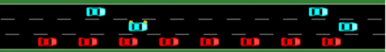
Figure 2: A highway segment with a platoon and interfering vehicles. To fix ideas consider Fig. 2, where we represent a platoon of 8 vehicles on a 3-lane motorway surrounded by other vehicles that also generate traffic. We focus on a vehicle in the platoon to give an example of a Cooperative Adaptive Cruise Control (CACC) system, but the modeling procedure is general and can be applied to any vehicle. A platoon member is interested in receiving packets from all the other vehicles in the platoon, and possibly also from other vehicles nearby, for instance the standard Cooperative Awareness Message (CAM) safety messages. However, considering a single packet, say from the platoon leader, all other frames that collide with this frame must be considered as interference, and since the “useful” packets may arrive from any vehicles, we should include the total number of vehicles within hearing range into the state of the model. The number of vehicles is not enough to characterize the potential interference, though. We have to consider the distance or reception power, too. Unlike the number of vehicles, the reception power is a continuous variable and does not map well to a Markov state variable. However, due to the randomness of propagation, shadowing, and fading, there is no reason to consider exact power levels, as it is not possible to characterize the exact power of interference received from a specific vehicle. Thus we can quantize the power level and obtain power classes (or distances, as the transmitting power is constant). Interfering vehicles are assigned to these classes.
Finding the optimal number of classes is outside the scope of this paper. Instead, we consider three simple classes based on distance and the expected receiving power in a free space propagation model: vehicles within 100 m from the receiver (class 1), between 100 m and 400 m (class 2), and beyond 400 m but above the noise floor (class 3), or equivalently in dBm the thresholds are roughly, −66, −78, with a transmission power of 20 dBm. These thresholds are arbitrary and they correspond to “zones of interest”, i.e., vehicles very close to the receiver and thus very interesting, vehicles with potentially interesting information because they are close enough, and all the others that may still add to interference. Furthermore, these thresholds correspond to power levels that are meaningful for channel capture phenomena when a packet received from the platoon is considered (again refer to Fig. 2): interfering packets from class 1 vehicles most likely destroy the packet of interest, those from class 2 may destroy it but with low probability, and those from class 3 will most likely be just additional noise and the packet of interest is received.
Following this reasoning, we can describe the state of the model with the 3-ple describing the number of vehicles in each
class: s = (n1, n2, n3). The extension to more classes is trivial
and the power thresholds defining the classes can be tuned to optimize the model performance.
The structure of the state selected leads by construction to a
(1, 0) (2, 0) (3, 0) (0, 1) (1, 1) (2, 1) (3, 1) ... ... (1,1)(0,1) ... ... ... (0,1)(1,1) (2,1)(1,1) (1,1)(2,1) (3,1)(2,1) (2,1)(3,1) ... (2,0)(1,0) (1,0)(2,0) (3,0)(2,0) (2,0)(3,0)
Figure 3: The initial part of BDP Markov Chain with only two power states that modulates the AoI generation process.
semi-Markov chain with Birth-Death Process (BDP) structure as represented in Fig. 3. This example uses only two power
classes to visualize the concept; the state is thus s = (n1, n2).
The chain is semi-Markovian because the evolution of the system depends only on the state at the moment of observation, but it cannot be proved (and it is indeed not true) that the dwell time is exponential. Assuming that dwell times, and hence transition rates, are exponentially distributed is instead an approximation that can be done for analytic tractability, but whose impact on the properties of the model has to be evaluated. The statement that the evolution of the system depends on the state only stems from the observation that the probability of a vehicle entering/exiting the space of interference, or changing interference class, can only depend on the number of vehicles in the space of interference at the present moment. It cannot depend on how many of them were present in the past, as this would imply a that a non-observable variable (the vehicle is not present now) influences the behavior of the system.
By construction of the model, the number of interfering vehicles is updated only when packets are received, so that the only transitions allowed are:
(··· , nk, ···) → (··· , nk+ 1, ···)
(··· , nk, ···) → (··· , nk− 1, ···)
(··· , ni, ··· , nj, ···) → (··· , ni− 1, ··· , nj+ 1, ···)
(1)
in the case of three considered classes with k, i, j ∈ (1, 2, 3) and in general depending on the number of power classes. It is useful to highlight that state (0, 0, 0) is impossible, because without vehicles within hearing distance there are no packets received and no information that can age.
The AoI for cooperative driving can thus be represented by a semi-Markov modulated process with a BDP structure, which is an important step in understanding AoI in this scenario. Unfortunately, as we discussed in the introduction, the Probability Density Function (pdf) of AoI is complex and cannot be approximated by a Poisson Process. Thus even assuming exponential dwell times, it is not possible to consider a simple Markov Modulated Poisson Process (MMPP) model. The remaining part of this section is dedicated to present the data needed to characterize the model.
A. Tuning the Model and Estimating AoI Distribution
To tune the model we evaluate the rates αs,d of the possible
every existing power state. We do this using a simulator as ground truth as explained in detail in Sect. III. Concerning
the transition rates αs,d, we collect all transition time samples,
so that the complete semi-Markov process can be estimated. The simulation measures each transition event, so that the rate averages are computed using the sample mean of the transition times: αs,d= " 1 ns,d ns,d X i=1 ts,d(i) #−1 (2)
where ns,d is the number of transitions between states s and d
during the simulation and ts,d(i) is the i-th sample of the time
spent in state s before the transition to state d. The transitions that entail adding a new interfering vehicle or moving an interfering vehicle from one power class to another are triggered by the reception of a packet from that vehicle. Clearly this cannot capture transitions that imply the reduction of interfering vehicles. The death process is modeled as a random negative exponential variable with average 1 s from the last reception of a packet from a vehicle, thus these transitions are Markovian by construction; 1 s is an arbitrary value coherent with the 100 ms beaconing interval of CAMs.
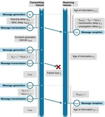
Modeling and tuning the AoI pdf is more complex. Let’s refer again to Fig. 1 and do this in light of the description of how AoI accumulates since the generation of a message.
Queuing delay dq,i + MAC delay dMAC,i dq,i+1 + dMAC,i+1 dq,i+2 + dMAC,i+2 dtotal,j = dq,i + dMAC,i + transmission delay dt,i + propagation delay dp,i
Message transmission ttx,i+2
Message transmission ttx,i+1
Message transmission ttx,i
Transmitting
Vehicle ReceivingVehicle
Age of information uj Constant generation interval tsent Packet loss lj Age of information uj+1 Age of information uj-1 tsent tsent Message reception Message reception trx,j
Message generation tg,i+2
Message generation tg,i+1
Message generation tg,i
trx,j+1 dtotal,j+1
Figure 4: Message sequence chart showing the AoI of a CAM message transmission sequence with one intermediate loss lj= 1.
Let uj be the AoI at the receiver relative to the received
message j, and dtotal,jbe the total delay of the communication
stack of successful transmission j, respectively any transmission attempt i. The counters i of transmission attempts and j of successful receptions are kept separate, as losses on the channel
affect the counter j but not i. As shown in Fig. 1, uj grows
linearly starting from the time of the reception of message j − 1 until the reception of message j. Considering now Fig. 4 that describes the time sequence of sending and receiving CAMs
we can derive the total delay dtotal,j= dq,i+ dM AC,i+ dt,i+
dp,i, with queuing delay dq,i, channel access delay dM AC,i,
transmission delay dt,i, and propagation delay dp,i. Considering
the latest successful transmission j, for any time instance t the AoI is formally defined as
u(t) = t − trx,j+ dtotal,j. (3)
For a well designed communication system (e.g., no head-of-the-line blocking and old information replaced by new one
so that dq,i ≤ tsent, ∀i), the AoI distribution is dominated
by the loss process, i.e., by interference, which is exactly the information we embed in the semi-Markov modulated process.
III. SIMULATION ANDDATACOLLECTION
To perform the data collection for the characterization of the
AoI model, we setup a simulation scenario in PLEXEversion
3.0-alpha1 [5]. PLEXEis an Open Source framework extending
the Veins [6] vehicular networking simulator and the SUMO mobility simulator with platooning capabilities.
In particular, we design a scenario with an 8-vehicle platoon and a variable number of human-driven vehicles that may interfere. The platoon is driven by the California PATH CACC, except for the leading vehicle that is driven by a standard Adaptive Cruise Control (ACC). The inter-vehicle spacing in the platoon is set to a fixed distance of 5 m and the platoon drives at a constant speed of 100 km/h. The human-driven vehicles, instead, are controlled by the Intelligent Driver Model (IDM) included in SUMO, and each vehicle has a random desired speed that is distributed according to a truncated Gaussian, so that 95 % of the vehicles drive within the 80 % and the 120 % of the speed limit, which is set to 130 km/h. This enables a time-varying scenario permitting the collection of enough data to analyze the AoI in a large area of the state space.
With respect to communication, the platooning vehicles exchange control information of 200 B in size periodically, with an update rate of 10 Hz. The human-driven vehicles also send beacons at the same rate generating interference. The chosen transmit power is 20 dBm and the rate is 6 Mbit/s.
To characterize communication delays and the loss process, each beacon sent by a platoon member is marked with a timestamp indicating when the information is generated and an incremental sequence number. During the simulation, this information is used to compute the communication delays, as well as the number of missing packets. This information is stored, for each received packet, with the reception time. More formally, each correct reception event generates a tuple in the output file (t, Vtx, Vrx, δtotal, Nlost), where t is the reception
time, Vtx and Vrx are the transmitter and the receiving vehicle
IDs, respectively, δtotal is the total communication delay (i.e.,
reception time minus generation timestamp), and Nlost is the
number of packets lost in between.
To characterize transitions in the state space, each platooning member maintains a table of neighbors. For each received
0 0.05 0.1 0.15 0.2 0.25 0.3 0.35 Age of Information [s] 0 0.2 0.4 0.6 0.8 1 CCDF State s=(11,20,72), N=100 State s=(07,01,09), N=10 0 1 2 3 4 5 6 7 8 transition time [s] 10-3 10-2 10-1 100 CCDF (07,01,09) (07,01,08) (11,20,73) (11,20,72) mean transition time
Figure 5: Complementary Cumulative Distribution Function (CCDF) of 8-cars platoon with 10 and 100 additional cars. Top plot: AoI values, each line representing the distribution within one state. The two states occurring the most are highlighted in blue (10 more cars) and green (100). Bottom plot: transition times in the same scenario; the two most-occurring transitions are highlighted in blue and green. packet the receiver extracts the sending vehicle ID and received power and updates its neighbors table. Each reception is logged
as a tuple (t, Vtx, Vrx, Prx) to compute state transitions during
the post processing phase, Prx is the received power. Each
time a packet is received, a negative exponential timer with average 1 s is started and, if no packet from the same receiver is received within this time, the neighbor is removed and the event logged.
The data collected in this initial scenario is shown in Fig. 5 both for the case of 10 and 100 human driven vehicles, leading to 17 and 107 interfering cars respectively. The top plot shows the AoI measured in every state, while the bottom plot reports the transition times for all possible transitions in the model. Results for the most probable states and most probable transitions, respectively, are highlighted in blue and green for the 10 and 100 interfering cases, respectively. Despite the difference in interfering vehicles, all states show similar AoI distributions in line with what can be expected with these interfering scenarios, i.e., very rarely packets are lost, and almost never are two of them lost in a sequence. Even if the simulations collected a few millions events, the result confidence of the AoI distribution is still limited. Yet it is clear that cooperative driving applications can be designed based on the worst case AoI of the semi-Markov state which represents the expected worst high-interference environment.
The bottom plot in Fig. 5 shows the transition time distribu-tions in semi-log scale. The figure validates the assumption that state transition rates depend on the environment and vehicle mobility in the scenario: the more interfering vehicles there are surrounding the platoon, the more frequently there are
changes in received transmission powers and thus the faster are the transitions. The vertical dotted lines mark the average of the highlighted transitions of the relative scenario (10 and 100 interfering vehicles). At a first, heuristic inspection, the transition rates seem to be roughly exponentially distributed, thus justifying an approximation with a Markov Modulation (MM) process, especially in the cases with a lot of interference; however, besides their exponential distribution, what needs to be verified to justify a MM process is the independence of samples, which is part of our future work. With many interfering vehicles state transitions are extremely fast, corresponding to the emission of just a few beacons per vehicle, which may have an impact on the characterization of the AoI distribution.
IV. FUTUREWORK
We have presented an initial effort to find a model that can generate samples of the AoI in an efficient way to design cooperative driving applications. We showed that a semi-Markov model based on the number of interfering vehicles seems to suffice to achieve this goal, although limited time and space prevented to explore a meaningful set of scenarios. Future work include several steps. First of all the generation of enough simulation experiments to properly tune the model in different scenarios and to find an appropriate expression for the AoI pdf. Next, the solution of the model (i.e., finding the steady state of the modulating process in the assumption of exponential dwell times) will provide a means to generate samples of AoI estimating the approximation introduced assuming that the process is pure Markov and not semi-Markov. Then, the model can be used either to drive ultra-fast simulations (we expect that generating AoI samples through the model will be several orders or magnitude faster than running a detailed event-driven simulation). Finally, the pure Markov model, with additional approximations, can be used to perform the analytic design of platoon controllers, consensus algorithms for collision avoidance, and other cooperative driving applications.
REFERENCES
[1] A. Kosta, N. Pappas, and V. Angelakis, “Age of Information: A New Concept, Metric, and Tool,” Foundations and Trends in Networking, vol. 12, no. 3, 2017.
[2] S. Kaul, R. Yates, and M. Gruteser, “Real-time status: How often should one update?” in 31st Annual IEEE Int. Conf. on Computer Comm. (INFOCOM): Mini-Conference, Orlando, FL, USA, Mar. 2012. [3] L. Baldesi, L. Maccari, and R. Lo Cigno, “Keep It Fresh: Reducing the
Age of Information in V2X Networks,” in ACM TOP-Cars ’19, Catania, Italy, 2019.
[4] G. Giordano, M. Segata, F. Blanchini, and R. Lo Cigno, “The joint network/control design of platooning algorithms can enforce guaranteed safety constraints,” Elsevier Ad Hoc Networks, vol. 94, 2019.
[5] M. Segata, S. Joerer, B. Bloessl, C. Sommer, F. Dressler, and R. Lo Cigno, “PLEXE: A Platooning Extension for Veins,” in 6th IEEE Vehicular Networking Conference (VNC 2014). Paderborn, Germany: IEEE, 2014. [6] C. Sommer, R. German, and F. Dressler, “Bidirectionally Coupled Network and Road Traffic Simulation for Improved IVC Analysis,” IEEE Transactions on Mobile Computing, no. 1, 2011.