2020-08-21T14:54:25Z
Acceptance in OA@INAF
Abell 315: reconciling cluster mass estimates from kinematics, X-ray, and lensing
Title
BIVIANO, ANDREA; Popesso, P.; Dietrich, J. P.; Zhang, Y. -Y.; Erfanianfar, G.; et
al.
Authors
10.1051/0004-6361/201629471
DOI
http://hdl.handle.net/20.500.12386/26756
Handle
ASTRONOMY & ASTROPHYSICS
Journal
602
Number
DOI:10.1051/0004-6361/201629471 c ESO 2017
Astronomy
&
Astrophysics
Abell 315: reconciling cluster mass estimates from kinematics,
X-ray, and lensing
?
,
??
A. Biviano
1, P. Popesso
2, J. P. Dietrich
3, 2, Y.-Y. Zhang
4,†, G. Erfanianfar
2, 5, M. Romaniello
6, 2, and B. Sartoris
7, 11 INAF–Osservatorio Astronomico di Trieste, via G. B. Tiepolo 11, 34143 Trieste, Italy e-mail: [email protected]
2 Excellence Cluster Universe, Boltzmannstr. 2, 85748 Garching bei München, Germany 3 Faculty of Physics, Ludwig-Maximilians-Universität, Scheinerstr. 1, 81679 München, Germany 4 Argelander-Institut für Astronomie, Universität Bonn, Auf dem Hügel 71, 53121 Bonn, Germany 5 Max Planck Institut für Extraterrestrische Physik, Postfach 1312, 85741 Garching bei München, Germany 6 European Southern Observatory, Karl-Schwarzschild-Str. 2, 85748 Garching bei München, Germany 7 Dipartimento di Fisica, Università degli Studi di Trieste, via G. B. Tiepolo 11, 34143 Trieste, Italy
Received 4 August 2016/ Accepted 10 February 2017
ABSTRACT
Context. Determination of cluster masses is a fundamental tool for cosmology. Comparing mass estimates obtained by different probes allows to understand possible systematic uncertainties.
Aims.The cluster Abell 315 is an interesting test case, since it has been claimed to be underluminous in X-ray for its mass (determined via kinematics and weak lensing). We have undertaken new spectroscopic observations with the aim of improving the cluster mass estimate, using the distribution of galaxies in projected phase space.
Methods.We identified cluster members in our new spectroscopic sample. We estimated the cluster mass from the projected phase-space distribution of cluster members using the MAMPOSSt method. In doing this estimate we took into account the presence of substructures that we were able to identify.
Results. We identify several cluster substructures. The main two have an overlapping spatial distribution, suggesting a (past or ongoing) collision along the line-of-sight. After accounting for the presence of substructures, the mass estimate of Abell 315 from kinematics is reduced by a factor 4, down to M200 = 0.8+0.6−0.4× 10
14M
. We also find evidence that the cluster mass concentration is unusually low, c200 ≡ r200/r−2 . 1. Using our new estimate of c200we revise the weak lensing mass estimate down to M200 = 1.8+1.7−0.9× 10¹⁴M
. Our new mass estimates are in agreement with that derived from the cluster X-ray luminosity via a scaling relation, M200= 0.9 ± 0.2 × 10¹⁴M .
Conclusions.Abell 315 no longer belongs to the class of X-ray underluminous clusters. Its mass estimate was inflated by the presence of an undetected subcluster in collision with the main cluster. Whether the presence of undetected line-of-sight structures can be a general explanation for all X-ray underluminous clusters remains to be explored using a statistically significant sample.
Key words. galaxies: clusters: individual: Abell 315 – galaxies: kinematics and dynamics
1. Introduction
Accurate and precise determination of galaxy cluster masses is of crucial importance for cosmological studies (e.g.,
Sartoris et al. 2012, 2016). Cluster masses can be determined from scaling relations with other cluster properties (see, e.g.,
Kravtsov & Borgani 2012), such as the X-ray luminosity (LX;
see, e.g., Popesso et al. 2005; Rykoff et al. 2008) and tem-perature (TX; see, e.g., Arnaud et al. 2005), the optical or
near-infrared luminosity (e.g.,Popesso et al. 2005;Mulroy et al. 2014), the velocity dispersion and velocity distribution of mem-ber galaxies (e.g., Munari et al. 2013; Ntampaka et al. 2015), and the Sunyaev-Zel’dovich signal (e.g., Sereno et al. 2015). Direct measurements of cluster masses can be obtained by
?
Based in large part on data collected at the ESO VLT (prog. ID 083.A-0930).
?? Full Table 1 and a Table of the measured redshifts and galaxy positions are only available at the CDS via anonymous ftp to
cdsarc.u-strasbg.fr(130.79.128.5) or via
http://cdsarc.u-strasbg.fr/viz-bin/qcat?J/A+A/602/A20
†
Deceased.
assuming hydrostatic equilibrium of the X-ray emitting intra-cluster gas (e.g.,Rasia et al. 2006), by the measurement of grav-itational lensing shear and magnification (e.g., Umetsu et al. 2014), and by the analysis of projected phase-space distribution of cluster galaxies (see, e.g., the review byBiviano 2008, and references therein), the so-called “kinematic” mass estimate.
All these methods suffer from possible systematics, aris-ing both from observational biases, and from violataris-ing the as-sumptions on which the theoretical derivation of the system mass is based. X-ray mass estimates can be biased by gas bulk motions and the complex thermal structure of the X-ray emit-ting gas (Rasia et al. 2006), lensing mass estimates by the un-known source redshift (z) distribution (but not for low-z clus-ters) and the assumed concentration of the mass distribution (Hoekstra et al. 2015). Triaxiality (Corless & King 2007), mis-centering (Johnston et al. 2007), and substructures can affect both lensing mass estimates (Giocoli et al. 2014), and kinematic mass determinations (Biviano et al. 2006;Mamon et al. 2013).
A renewed interest in this topic has come from the puz-zling discrepancy between the values of the cosmological
parameters inferred from cluster counts in the Planck survey and from the primary cosmic microwave background anisotropies (Planck Collaboration XX 2014). A mass bias of 40% has been suggested to put the two measurements into agreement.
von der Linden et al.(2014) found the X-ray based Planck clus-ter mass estimates to be biased low by 30% compared to weak-lensing mass estimates. Their result might not however apply in general. Other studies have found good (e.g.,Israel et al. 2014;
Smith et al. 2016), if not excellent (e.g., Umetsu et al. 2012) agreement between lensing and X-ray mass estimates of clus-ter masses. The comparison of mass estimates from kinematics, with those from lensing and X-ray, have shown excellent agree-ment in some cases (e.g.,Biviano et al. 2013), and serious dis-crepancies in others (e.g.,Guennou et al. 2014).
The fact that for some clusters different techniques lead to consistent mass estimates, and for some they do not, might be related to the dynamical status of these clusters.Popesso et al.
(2007, P07 hereafter) claimed the existence of a class of X-ray underluminous clusters, which would explain the matching dis-crepancies between cluster samples extracted from X-ray and from optical surveys (Donahue et al. 2002;Gilbank et al. 2004;
Basilakos et al. 2004;Sadibekova et al. 2014). The matching ap-pears to be better between cluster samples extracted from optical and from Sunyaev-Zel’dovich (SZ) surveys (Rozo et al. 2015). Merging clusters may account for the poor matching between optical and X-ray detected clusters. In fact, in merging clusters the peak of the mass distribution is offset from the peak of the X-ray emission, as seen in the Bullet cluster (Markevitch et al. 2002), but not from the peak of the SZ signal (Zhang et al. 2014). Moreover, X-ray cluster surveys are biased in favor of high-central density, cool-core clusters (Eckert et al. 2011), and mergers can disrupt a cluster cool-core and reduce the concen-tration of diffuse baryons relative to that of the dark matter (Roettiger et al. 1996;Burns et al. 2008;Poole et al. 2008).
Bower et al.(1997) argued that low-LXclusters of high
rich-ness and velocity dispersion (σv) are systems of galaxies
em-bedded in large-scale filaments oriented along the line-of-sight.
P07 noted that these clusters (which they called “AXU” for “Abell X-ray underluminous”) are characterized by a relative low density of galaxies near their core and a higher fraction of blue galaxies, relative to normal X-ray emitting clusters. These characteristics could suggest line-of-sight contamination. On the other hand,P07were unable to find dynamical evidence for sub-structure in excess of what was found in normal clusters. Sig-nature for significant mass infall rates in the external regions of the AXU clusters was found, based on the shape of their galaxy velocity distribution.
To highlight the nature of the low-LX or high σv of AXU
clusters, Dietrich et al. (2009, D09 hereafter) determined the weak lensing masses of two such clusters, Abell 315 and Abell 1456 (A315 and A1456 hereafter), at z = 0.174 and 0.135, re-spectively.D09could only set an upper limit to the weak lens-ing mass of A1456, which was significantly below the kine-matic mass estimate, but consistent with the mass predicted from the cluster LX. The velocity distribution of member galaxies in
A1456 was found to be very skewed or even bimodal, sugges-tive of a complex dynamical structure that could have biased the kinematic mass estimate high. The X-ray underluminous nature of A1456 could therefore be rejected.
D09’s weak lensing mass estimate of A315, on the other hand, was found to be consistent with the one determined from kinematics, but about three times larger than the mass expected from the cluster LX using the scaling relation of Rykoff et al.
(2008). A315 thus remained a good AXU candidate.
To gain insight into the nature of this cluster, we obtained al-most 500 redshifts for galaxies in the cluster field, of which '200 are estimated to be cluster members. In this paper we present these new data, that we use to investigate the internal structure of A315, and re-determine its kinematic mass estimate. In Sect.2
we describe our dataset, in Sect.3we identify the cluster mem-bers, in Sect.4we search for the presence of substructures, and in Sect.5 we determine the cluster mass from kinematics. We discuss our results in Sect. 6 and provide our conclusions in Sect.7.
We use H0= 70 km s−1Mpc−1,Ω0= 0.3, ΩΛ= 0.7
through-out this paper. In this cosmology, at the cluster mean redshift, z = 0.174, 1 arcmin corresponds to 0.178 Mpc. All errors are quoted at the 68% confidence level.
2. The dataset
Abell 315 was observed at the European Southern Observatory (ESO) Very Large Telescope (VLT) with the VIsible MultiOb-ject Spectrograph (VIMOS;Le Fèvre et al. 2003). The VIMOS data were acquired using 8 separate pointings, plus 2 additional pointings required to provide the needed redundancy within the central region and to cover the gaps between the VIMOS quad-rants. Each mask was observed for 1.5 h, for a total of 15 h ex-posure time. The HR-Blue grism was used, covering the spec-tral range 415–620 nm with a resolution R ∼ 2000. We have reduced the data with the ESO data processing pipeline v2-9-141. Raw science frames were corrected for bias and flat-field and calibrated in wavelength according to the standard in-strument calibration plan2. Flux calibration was derived from nightly flux standard star observations. The flux standard stars themselves were processed following the same steps as science frames and the resulting response curve was, then, applied to the processed science spectra. In order to automatize data process-ing, we have assembled the pipeline recipes in a Reflex workflow (Freudling et al. 2013). Redshift estimation has been performed by cross-correlating the individual observed spectra with tem-plates of different spectral types fromPolletta et al.(2007). Tem-plates for ordinary S0, Sa, Sb, Sc, and elliptical galaxies were used to measure redshifts of relatively low redshift galaxies. The cross-correlation is carried out using the rvsao package (xcsao routine,Kurtz & Mink 1998) in the Image Reduction and Anal-ysis Facility (IRAF) environment. The final sample comprises 479 reliable redshifts in the heliocentric rest-frame.
Additional redshifts (in the heliocentric rest-frame) for galaxies in the cluster area were taken from the Sloan Digital Sky Survey (SDSS) III (Eisenstein et al. 2011;Ross et al. 2014) DR10, 499 in total. There are 32 objects in common to our spectroscopic sample and the SDSS. For one of them there is a substantial difference in the two redshift estimates. The VIMOS redshift estimate is however quite uncertain. It was based on a spectrum that looks significantly noisier than the SDSS one, pos-sibly because of an imperfect slit centering on the galaxy, due to the VIMOS focal plane distortion. For the remaining 31 we evaluate a mean redshift difference of −1.7 × 10⁻⁴, and a
dis-persion of 4.4 × 10⁻⁴. We use this value and the average un-certainty of the SDSS redshifts, to estimate an average uncer-tainty of ∼110 km s−1for the cluster rest-frame velocities of our VIMOS spectroscopic sample. The VIMOS velocity uncertainty 1 VLT-MAN-ESO-19500-3355,ftp://ftp.eso.org/pub/dfs/
pipelines/vimos/vimos-pipeline-manual-7.0.pdf
2 http://www.eso.org/sci/facilities/paranal/
Fig. 1.Histogram of redshifts in the cluster area. The red, hatched his-togram shows galaxies with redshifts within ±0.016 of z = 0.174, the mean cluster redshift according toP07.
is larger than the average uncertainty of the SDSS velocities, ∼30 km s−1, so we choose the SDSS redshift estimate rather than our own, when both are available for a given galaxy.
Magnitudes and positions for galaxies in the cluster field were gathered from the SDSS DR10.
In total our sample contains 946 galaxies with at least one redshift estimate in the cluster field, over an area of 1◦120× 450. The z-distribution of all galaxies in our spectroscopic sample is shown in Fig.1. There is a prominent peak at the mean cluster redshift, z= 0.174 (P07).
The spectroscopic sample is presented in Table1. In Col. (1) we list a galaxy identification number, in Cols. (2) and (3) the galaxy right ascension and declination (J2000), in Cols. (4) and (5) the redshift estimate from SDSS, and from our VIMOS observations respectively, when available, in Col. (6) we flag cluster members (for the determination of cluster membership see Sect.3), in Col. (7) we flag members in substructures iden-tified by the DSb technique (see Sect. 4 and AppendixA). In Col. (8) we list the probability of a member in the virial region of the cluster, and outside DSb-type substructures, to belong to the KMM-main subcluster (see Sect.4).
3. Cluster membership
To define which galaxies are members of the cluster we use their location in projected phase-space R, vrf, where R is the projected
(respectively 3D) radial distance from the cluster center (that we need to identify) and vrf ≡ c (z − z)/(1+ z), is the rest-frame
velocity and z is the mean cluster redshift.
Following Beers et al. (1991) and Girardi et al. (1993) we first identify the cluster main peak in redshift space, by se-lecting the 252 galaxies with rest-frame velocities in the range ±4000 km s−1, that is within ±0.016 of the mean cluster redshift (see Fig.1).
To define the center of the cluster we cannot rely on the peak of the X-ray emission, because of poor photon statis-tics (D09). D09 noticed that the weak lensing peak of A315 was close to a local galaxy overdensity, and they chose the brightest galaxy of this overdensity as the cluster center. How-ever, this galaxy does not appear to be the brightest cluster galaxy, as can be seen in Fig.2. In this figure we plot the clus-ter members (as defined below) as circles with sizes propor-tional to 1/(mR− 16.5), where mR are the galaxy red apparent
Fig. 2.Positions of the cluster members with respect to the peak of their projected number density (the center is at αJ2000= 2h10m15s.0, δJ2000= −1◦
20
3100.0). North is up and east is to the left. Galaxy positions are indi-cated by circles with sizes proportional to 1/(mR− 16.5), where mRare the galaxy red apparent magnitudes. Red (respectively blue) circles identify galaxies with vrf≥ −677 km s−1(respectively <−677 km s−1), a limit that separates galaxies in the KMM-main subcluster from galaxies in the KMM-sub subcluster (see Fig.6in Sect.4). The galaxy selected byD09as the cluster center is indicated by a blue, cyan-filled, circle at {x, y} = {−2.1, 0.7}. The purple circle has a radius of 1.24 Mpc and it indicates the cluster virial region (see text).
magnitudes. Red (respectively blue) circles identify galaxies with vrf≥ −621 km s−1(respectively <−621 km s−1), a limit that
separates galaxies in the KMM-main subcluster from galaxies in the KMM-sub subcluster (see Fig.6in Sect.4). The galaxy selected as the cluster center by D09is part of the KMM-sub subcluster (that we identify in Sect. 4) and is not the brightest cluster galaxy in the central cluster region.
Since we can define the cluster center neither from its X-ray emission nor from the position of a dominant galaxy, we use as a center the peak of the projected number density of clus-ter galaxies, that we declus-termine as follows. We consider the 2D projected spatial density distribution of cluster members, after correcting our spectroscopic sample for spatial incompleteness, since some regions are better covered by spectroscopic observa-tions than others. To correct this sample for incompleteness, we rely on a sample with homogeneous spatial coverage, that is the sample of photometric members defined by using the photomet-ric redshifts (zphot) from SDSS.
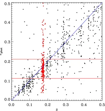
In Fig.3we show the correlation between zphotand the
spec-troscopic redshift z, for the 913 galaxies which have both es-timates (we restrict the plot to the redshift range 0–0.5). We followKnobel et al.(2009) and select the zphotrange that
min-imizes the metric p(1 − P)2+ (1 − C)2, where P, C denote the
purity and completeness of the photometric sample of selected members relative to the sample of 252 spectroscopic members selected in the main redshift peak. This metric reaches a mini-mum at C = 0.72, P = 0.59 for the zphot range 0.113–0.211, a
range we adopt to select 2327 photometric members.
Of all the selected photometric members, we only consider the 819 brighter than zPetro≤ 19.64 (corresponding to a
Table 1. Spectroscopic dataset.
Id αJ2000 δJ2000 zSDSS zVIMOS Member Subst Prob
2 2h07m36s.01 −0◦5900400. 7 0.6056 – – – – 164 2h07m40s.54 −1◦1004300. 7 – 0.1768 M – – 328 2h07m44s.40 −0◦3804500. 3 0.1748 – M – – 3272 2h09m06s.76 −0◦5904100. 5 0.3732 0.3719 – – – 3664 2h09m53s.21 −1◦0004600. 0 – 0.1734 M – 0.98 3667 2h10m00s.91 −0◦5901200. 0 0.1701 – M – 0.07 6437 2h10m35s.72 −0◦5004500. 6 0.1785 – M S –
Notes. The average uncertainties in the VIMOS and SDSS redshifts are 3.7 × 10⁻⁴ and 1.0 × 10⁻⁴, respectively. An “M” in the “Member” column identifies cluster members (identified as described in Sect.3), and an “S” in the “Subst” column identifies galaxies belonging to DSb-type substructures (see Sect.4and AppendixA). The “Prob” column lists probabilities of belonging to the KMM-main subcluster (see Sect.4). Only a portion of the Table is shown here, the full Table is available in at the CDS.
Fig. 3.Photometric vs. spectroscopic redshift estimates for galaxies in the cluster area. Red dots identify galaxies in the main redshift peak of Fig.1. The blue line represents the zphot= z identity. The two hori-zontal red lines represent the zphotlimits that we adopt to define cluster members for galaxies without z.
limit down to which the total number of galaxies with z is >1/4 of the total number of galaxies with zphot. We determine the map
of spectroscopic completeness by taking the ratio between the number of spectroscopic members and the number of photomet-ric members in bins of RA, Dec. We then assign a completeness value to each galaxy in the spectroscopic sample and in the cho-sen magnitude range, according to the galaxy position.
We have 147 spectroscopic members with zPetro≤ 19.64 and
with an assigned spectroscopic completeness >1/4, and we use this sample to construct an adaptive kernel map of the num-ber density of galaxies in the cluster region, by weighting each galaxy by the inverse of its completeness value. The resulting map is shown in Fig.4, and is centered on the point of maximum density, located at αJ2000 = 2h10m15s.0, δJ2000 = −1◦203100. 0.
This is the center we adopt for A315. Our adopted center is 0.39 Mpc away from the position adopted byD09, that was used
Fig. 4.Adaptive-kernel map of the number density of cluster members with magnitude zPetro≤ 19.64, corrected for incompleteness of the spec-troscopic sample. Darker shadings indicate higher densities, logarith-mically spaced. The red dots identify all galaxies which are identified as cluster members by the SG algorithm (see Sect.3). The green dots identify the galaxies flagged by the DSb procedure (described in Ap-pendixA) as possible members of substructures. The green polygon indicates 10 of these galaxies that appear to form a compact group (the “DSb group”). The map is centered at the point of maximum projected number density of cluster galaxies, as in Fig.2(also indicated by a yel-low plus sign). North is up and east is to the left. The yelyel-low diamond symbol identifies the position of the galaxy used as a cluster center in
D09. The purple circle has a radius of 1.24 Mpc and indicates the cluster virial region (see Sect.3).
as a center for the Navarro, Frenk, & White (NFW,Navarro et al. 1997) profile fitting of the weak lensing map.
Once we have defined the cluster center, we can proceed to a better identification of the cluster members, by making use not only of the velocity of galaxies but also of their spatial distribu-tion in the cluster region. We use the shifting-gapper (SG) algo-rithm ofFadda et al.(1996) to identify cluster members in pro-jected phase-space, using a velocity gap size of 1000 km s−1, a spatial bin size of 500 kpc, and a minimum of 15 galaxies per spatial bin, as indicated byFadda et al.(1996). We identify 222 cluster members by this method, that is we reject 30 galaxies among those belonging to the main redshift peak. The location of the 222 selected members in the cluster area is shown in Fig.4
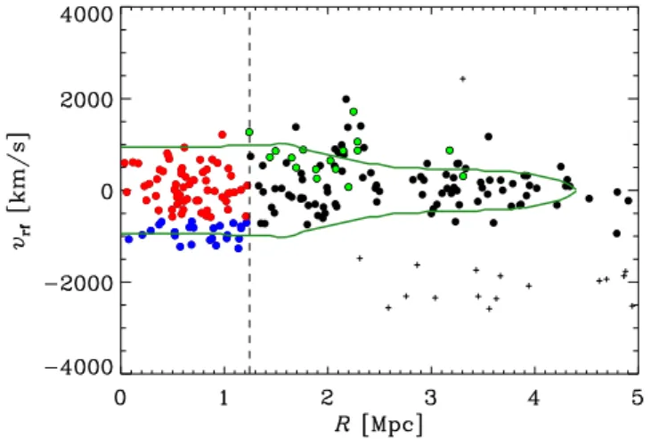
Fig. 5.Projected phase-space distribution of galaxies in the cluster field, vrfvs. R. Crosses and dots represent interlopers and cluster members, respectively, identified by the SG algorithm ofFadda et al.(1996). The vertical line is a preliminary estimate of the cluster r200(rσ200) based on the global estimate of the cluster velocity dispersion (see Sect.3). Mem-bers within r200σ are identified with blue (respectively red) dots, if they have a probability ≥0.5 to belong to the sub (respectively KMM-main) subcluster identified by the KMM algorithm (see text and Fig.6,
McLachlan & Basford 1988;Ashman et al. 1994). The green colored dots indicate those members that are flagged by the DSb procedure (described in AppendixA) as possible members of substructures. The green curves represent the Caustics identified by the Caustic technique ofDiaferio & Geller(1997) (see Sect.5.2).
and in projected phase-space in Fig.5. Hereafter we refer to the sample of 222 cluster members as the “Total sample”.
We check our membership definition using the “Clean” al-gorithm of Mamon et al. (2013). Using the “Clean” algorithm the number of selected members is 208. Differences in the two member selection algorithms concern only galaxies located at distances >1 Mpc from the center. In the rest of the paper we present the results based on the SG membership selection, since the Clean algorithm is based on the assumption that the clus-ter mass profile follows a NFW distribution with a well defined theoretical mass-concentration relation. The SG algorithm is in-stead model-independent. Given that we investigate A315 be-cause of its special properties, we want to avoid biasing the re-sults by imposing typical characteristics of normal clusters. We checked that the results of this paper are not significantly depen-dent on the choice of the membership algorithm.
The mean redshift and velocity dispersion of the cluster members, evaluated using the biweight (Beers et al. 1990), are z = 0.1744 ± 0.0001, and σv = 603+29−31 km s
−1 (see also
Table2). We use this estimate of σv to get a preliminary
esti-mate of the cluster virial radius3, r
200, that we denote rσ200. To
estimate r200σ we follow the iterative procedure ofMamon et al.
(2013), where we assume an NFW model (Navarro et al. 1997) for the mass distribution, with a concentration given by the concentration–mass relation ofMacciò et al.(2008), and we as-sume the Mamon & Łokas (2005) velocity anisotropy profile with a scale radius identical to that of the mass profile. We find rσ200= 1.24 ± 0.06 Mpc. There are 89 members within rσ200. 3 The radius r
∆is the radius of a sphere with a mass overdensity∆ times the critical density at the cluster redshift. Throughout this paper we refer to the∆ = 200 radius as the “virial radius”, r200. Given the cosmological model, the virial mass, M200, follows directly from r200 once the cluster redshift is known, G M200 ≡∆/2 Hz2r
3
200, where Hzis the Hubble constant at the mean cluster redshift.
Table 2. Mean velocities and velocity dispersions.
Sample N v σv T I km s−1 km s−1 Total 222 0 ± 40 603+29−31 1.07 DSb group 10 584 ± 95 282+72−58 – No-DSb 205 −60 ± 40 573+28−29 1.05 Inner 88 −205 ± 66 613+48−44 0.88 KMM-main 63 73 ± 56 441+41−38 0.93 KMM-sub 25 −924 ± 39 189+29−25 0.94 Outer 117 28 ± 46 503+34−32 1.02
Notes. Values of the rest-frame mean velocity, the line-of-sight velocity dispersion, and the Tail Index (T I; see text) of the cluster as a whole and split in several subsamples, and of the detected substructures. The mean velocity and the velocity dispersion are computed using the ro-bust biweight estimator (Beers et al. 1990). N is the number of objects in each sample. There are 17 DSb galaxies, of which 10 form a group, indicated as “DSb group” in the Table. The “No-DSb” sample is ob-tained from the “Total” after removal of the 17 DSb galaxies. “Inner” and “Outer” are subsamples of “No-DSb”, separated in radial distance by the value of rσ200. “KMM-main” and “KMM-sub” are subsamples of “Inner”, identified with the KMM algorithm, and separated in velocity space by the value −621 km s−1.
4. Substructures
We consider the presence of substructures in the cluster by using the test ofDressler & Shectman(1988), modified as described in AppendixA. This test (DSb test hereafter) looks for local de-viations of the mean velocity and velocity dispersion from the global cluster values. We apply the DSb test to the sample of cluster members defined in Sect. 3. In total, 17 members are flagged for their significant deviation in velocity from the lo-cal mean. Of these, 10 form a compact group in projection (see Fig.4), that we call the “DSb group” hereafter. It has a mean velocity of 584 ± 95 km s−1in the cluster rest-frame, and a ve-locity dispersion of 282+72−58 km s−1 (see also Table 2), typical of the general population of galaxy groups (see, e.g., Fig. 3 in
Ramella et al. 1999). The DSb substructure galaxies (including the DSb group) are displayed in the projected phase-space plot of Fig.5.
After removing the 17 galaxies flagged by the DSb algo-rithm from the Total sample, we are left with 205 members, the “No-DSb” sample hereafter.
To investigate the presence of additional substructures that remain undetected by the DSb test, we apply the Kernel Mix-ture Model (KMM) algorithm (McLachlan & Basford 1988;
Ashman et al. 1994) to the distribution of rest-frame velocities of the remaining 205 cluster members. The KMM algorithm fits a user-specified number of Gaussian distributions to a dataset, and returns the probability that the fit by many Gaussians is sig-nificantly better than the fit by a single Gaussian. Each Gaussian fit corresponds to a putative substructure of the cluster. The al-gorithm also returns the probability for each galaxy to belong to any of these substructures. Cluster velocity distributions are known to resemble Gaussians (e.g.,Girardi et al. 1993), but not when substructures are present (e.g.,Beers et al. 1991), in which case the decomposition of the velocity distribution into multi-ple Gaussians provides a more appropriate fit to the data (e.g.,
Fig. 6.Velocity distribution of cluster members (after excluding galax-ies flagged by the DSb substructure analysis). Top panel: members within rσ200= 1.24 Mpc. The blue and red histograms identify the KMM partitions (namely, members with probability ≥0.5 and, respectively, <0.5 to belong to the low-velocity group, KMM-sub). The dotted (blue and red) curves are the two Gaussians with mean and velocity disper-sions obtained from the subsamples of the same colors. The dash-dotted magenta curve is the sum of the two Gaussians. The black dashed curve is the Gaussian with mean and velocity dispersion obtained from the full sample. Bottom panel: members outside rσ200 = 1.24 Mpc (histogram). The black dashed curve is the Gaussian with mean and velocity disper-sion obtained from the full sample.
We apply the KMM test to three samples, (i) the No-DSb sample; (ii) the subsample of 88 members with R ≤ rσ200(“Inner” subsample hereafter), and the subsample of 117 members with R> rσ200(“Outer” subsample hereafter). The KMM test indicates that the velocity distributions of both the No-DSb sample and the outer subsample are not significantly better fit with 2 Gaussians than with a single one. On the other hand, a 2-Gaussians fit to the velocity distribution of the inner subsample is significantly better than a single-Gaussian fit, with a probability of 0.05.
We show the velocity distribution of the inner subsample, separated according to the two KMM partitions, in the upper panel of Fig. 6, and the velocity distribution of the outer sub-sample in the lower panel of the same figure. We also show the Gaussians with averages and dispersions obtained from the bi-weight estimator (e.g.,Beers et al. 1990) applied to the different distributions. In the projected phase-space plot of Fig.5we use red and blue dots to distinguish the two groups identified by the KMM algorithm in the inner sample.
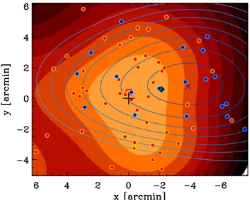
In Fig.7 we show the adaptive kernel density map of the galaxies in the two KMM groups – restricted to the virial re-gion where the two groups are defined. As before, we use com-pleteness weights to construct the map, and we only consider galaxies with zPetro ≤ 19.64 and with an assigned spectroscopic
completeness >1/4. We define the KMM-main and KMM-sub subclusters by considering galaxies of the inner subsample with vrf ≥ −621 km s−1 and vrf < −621 km s−1, respectively,
sepa-rated by the velocity value where the two best-fitting Gaussians intersect in Fig.6. The density peak of the spatial distribution of
Fig. 7.Adaptive-kernel maps of the number density of cluster mem-bers with magnitude zPetro≤ 19.64, corrected for incompleteness of the spectroscopic sample. Filled, red-orange contours represent the number densities of the KMM-main subcluster, open, blue-cyan contours repre-sent the number densities of the KMM-sub one. The red square and blue X identify the density peaks of the KMM-main and KMM-sub density maps, respectively. The contours are logarithmically spaced. The red (blue) dots identify member galaxies with velocity > −621 km s−1 (re-spectively ≤−621 km s−1) and are thus more (less) likely to belong to the KMM-main subcluster than to the KMM-sub one. The black cross identifies our adopted center of A315, from the analysis of the adaptive kernel density map of all members. The black diamond identifies the center used inD09.
the KMM-main subcluster is nearly coincident (0.07 Mpc sep-aration) with our adopted center for the whole cluster, as ex-pected given that 72% of the galaxies within rσ200belong to the KMM-main subcluster. The center of the KMM-sub subcluster, on the other hand, is 0.7 Mpc to the West of the cluster cen-ter. The center used byD09lies at intermediate distance along the line connecting the two group centers. The two groups over-lap substantially in the projected spatial distribution, and this overlap is suggestive of a past or ongoing collision close to the line-of-sight.
In Table2we list the values of the average velocities v and velocity dispersions σv, obtained with the biweight estimators,
for the different samples considered so far. The removal of the galaxies flagged by the DSb substructure analysis does not af-fect the v and σvvalues of the whole cluster significantly. In
par-ticular, σvdecreases by only 5% when we remove the 17
DSb-identified galaxies from the total sample. On the other hand, the σv of the Inner sample is significantly larger than those of the
two groups into which it is split by the KMM algorithm (by 28% and 69%).
In the same Table we also list the values of the Tail In-dex (T I) of the velocity distribution in each sample (except the DSb group, since 10 members are not enough for a reliable estimate of T I).Beers et al. (1991) have suggested the use of T I as a robust estimator of the shape of the velocity distribu-tion in galaxy clusters. Values of T I close to unity denote a Gaussian-like distribution, values >1 (respectively <1) a distri-bution with more (respectively less) galaxies at large velocity differences than expected for a Gaussian (leptokurtic and respec-tively platikurtic distribution).Popesso et al.(2007) have found that AXU clusters display on average a leptokurtic velocity
distribution at large radii, with T I = 1.45, and interpreted this evidence as suggestive of ongoing infall.
The values we find for the A315 cluster as a whole and for its different subsamples are not significantly different from unity, not even for the velocity distribution of members outside the virial region (see Table 2 inBird & Beers 1993, for the signif-icance levels of the T I). The velocity distribution within each KMM subcluster is closer to a Gaussian (T I = 0.93 and 0.94) than the full velocity distribution in the virial region (T I= 0.88). This difference of T I values is not significant, but taken at face value it gives further support to the existence of two subclusters in velocity space. Had we not excluded the galaxies flagged by the DSb algorithm from our sample, the T I value of the veloc-ity distribution of the Outer sample would increase from 1.05 to 1.08, which is also not significantly different from unity.
5. The mass estimate
We proceed to estimate the mass of the cluster by two techniques, MAMPOSSt (Mamon et al. 2013) and the Caustic (Diaferio & Geller 1997). In these estimates, when needed, we take into account the results of the substructure analysis of Sect. 4. In particular, in MAMPOSSt we remove the galaxies flagged by the DSb technique, and we weigh galaxies by their probability of belonging to the KMM-main subcluster. In the Caustic method we use the KMM-main subcluster σv to select
the relevant caustic.
5.1. MAMPOSSt
The MAMPOSSt technique has been developed by Mamon et al.
(2013). It determines the best-fit parameters (and their uncer-tainties) of models for the mass and velocity anisotropy profile of a system of collisionless tracers in dynamical equilibrium in a spherical gravitational potential. To do so, it performs a Max-imum Likelihood analysis of the projected phase-space distri-bution of the tracers, the member galaxies of the A315 cluster in our case. It has been tested with cluster-size halos extracted from cosmological simulations, by simulating a number of dif-ferent observational situations.
We use MAMPOSSt in the so called “Split” mode (see Sect. 3.4 inMamon et al. 2013), that is we separate the maximum Likeli-hood analyses of the spatial and velocity distributions of mem-ber galaxies. We prefer to use MAMPOSSt in the Split mode since our spectroscopic sample suffers from spatially inhomogeneous incompleteness, and while this spatial incompleteness affects the determination of the number density profile, it is unlikely to affect the observational determination of the distribution of velocities.
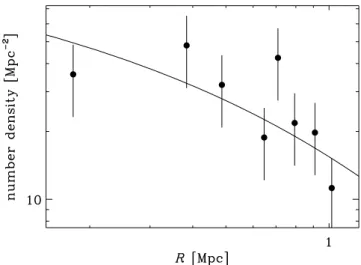
To estimate the number density profile we consider the same subsample of spectroscopically selected members that we used to derive the adaptive kernel map (Fig.4), restricted to the virial region, R ≤ rσ200. We fit a projected NFW model (Bartelmann 1996;Navarro et al. 1997) to the distribution of radial distances with a Maximum Likelihood technique, weighting the galaxies by the inverse of their completeness times their probability of be-longing to the KMM-main subcluster (see Sect.4). This weight-ing scheme is to ensure that we are modelweight-ing the KMM-main subcluster density profile, rather than that of the whole Inner sample of members. The best-fit model is shown in Fig.8. The best-fit NFW scale radius is rν= 1.0+0.7−0.3Mpc. The uncertainties
are large, but taking the result at face value it suggests a very low concentration of the galaxy distribution.
Fig. 8. Maximum likelihood best-fit of a projected NFW model (Bartelmann 1996;Navarro et al. 1997) to the distribution of radial dis-tances of the cluster members in the virial region and the binned number density profile with 1σ error bars. Only galaxies with zPetro≤ 19.64 and in regions of spectroscopic completeness >1/4 have been considered, and the sample has been corrected for incompleteness.
We then run MAMPOSSt on the Inner sample of members, by fixing the rν value at its best fit. We prefer to consider only galaxies within the expected virial region, to avoid including re-gions too far from virialization in the analysis. It has in fact been shown byMamon et al.(2013) that r200is the optimal choice for
minimizing the uncertainties in the parameter values obtained by MAMPOSSt. In calculating the likelihoods of the observed galaxy velocities, similarly to what we have done in the fit to the num-ber density profile, we weigh each galaxy in the sample by its probability of belonging to the KMM-main subcluster. Weigh-ing galaxies by their probabilities of belongWeigh-ing to the KMM-main subcluster is a way to account for the contamination by the KMM-sub subcluster, whose presumed members are assigned little (or zero) weight. We do not however use completeness as weights in the MAMPOSSt analysis, since the bias in the obser-vational selection of spectroscopic targets can easily affect the spatial distribution, but not the velocity distribution of cluster members.
In MAMPOSSt we search for the best-fit values of three free parameters:
1. The virial radius r200;
2. the scale radius of the mass distribution, that we choose to characterize by r−2, the radius at which d log ρ/d log r= −2,
where ρ(r) is the mass density profile;
3. a parameter that characterizes the velocity anisotropy profile, β(r) = 1 − σ2θ(r)+σ2φ(r) 2 σ2 r(r) = 1 − σ2 θ(r) σ2
r(r), where σθ, σφare the two
tangential components, and σr the radial component, of the
velocity dispersion, and we assume σθ= σφ.
We consider three models for the mass profile, M(r): 1)Burkert
(1995); 2)Hernquist(1990); and 3)Navarro et al.(1997) (Bur, Her, and NFW in the following). They are all characterized by two parameters, that we convert to r200and r−2when needed (see
Biviano et al. 2013, for a detailed description of these models). We consider four models for the velocity anisotropy pro-file, β(r): 1) a model with constant anisotropy at all radii, that we denote “C”; 2) the model of Mamon & Łokas(2005), that we denote “ML”; 3) the model ofOsipkov(1979) andMerritt
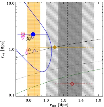
Fig. 9. Results for the M(r) parameters r200 and r−2. The blue con-tour indicates the 68% confidence level on the best-fit values obtained in MAMPOSSt (blue dot) for the best-fit models NFW+T (see text), af-ter marginalization over the anisotropy parameaf-ter. The horizontal solid blue segment indicates the error on the best-fit r200value, obtained after marginalization over the r−2and the anisotropy parameter. The best-fit results of other models are indicated by the open symbols, triangle, in-verted triangle, and circle, for the Bur, Her, NFW models, respectively, black, red, magenta, and blue for the combination with the C, ML, OM, and T models, respectively The size of the symbols is proportional to the relative likelihood of the models. The black cross indicates the mean [r200, r−2], taking the average over all models. The vertical, black dashed line indicate the r200value obtained byD09from their kinematic analy-sis. The uncertainties on this value, also taken fromD09, are indicated by shaded grey regions, where the pale grey shading includes both the statistical and the systematic uncertainties, while the dark grey shading only includes the statistical uncertainty. The vertical orange line and or-ange shading indicate the r200value and uncertainty obtained from the cluster LX(fromD09) using the scaling relation ofRykoff et al.(2008). The open maroon diamond indicates the r200 value obtained byD09 from their lensing analysis. The position along the y-axis indicates the r−2value corresponding to the assumed concentration r200/r−2used in
D09for the determination of the cluster lensing mass. The statistical and statistical+systematic uncertainties on this value are indicated by the maroon solid and dashed line, respectively. The filled gold diamond indicates the new determination of r200 from the lensing analysis ap-plied to the same data used inD09, but this time using a concentration r200/r−2= 1. This value of the concentration is used to set the position of the point along the y-axis. The dash-dotted green curve is the r−2vs. r200 relation derived from the concentration-mass relation of Correa et al.
(2015c) at the cluster redshift, computed with the code COMMAH (see also
Correa et al. 2015a,b). The triple-dot-dashed black curve indicates the r200= r−2relation. The dotted black curve indicates the c200= 2.9 rela-tion, namely the highest concentration that is still marginally acceptable according to the MAMPOSSt dynamical analysis.
Biviano et al.(2013). Using four different models for β(r) allows us to evaluate how much our results for M(r) are dependent on the poorly known form of β(r) in clusters of galaxies.
The best-fit of MAMPOSSt is obtained for the combination of the NFW and T models. All other models are statistically acceptable, at better than the 68% confidence level. In Table3
Table 3. MAMPOSSt results.
Parameter NFW+T models Mean of all models
r200[Mpc] 0.85+0.16−0.18 0.79 ± 0.02
r−2[Mpc] 2.1+6.5−1.0 1.6 ± 0.2
(σr/σθ)∞ 0.7+0.7−0.3 0.8 ± 0.1
Notes. The mean and associated errors have been computed using the biweight estimator (Beers et al. 1990). The “mean of all models” con-siders all 12 combinations of 3 models for M(r) and 4 models for β(r), except for the (σr/σ2θ)∞parameter, which is only defined for the T β(r) model.
we give the best-fit values and uncertainties of r200, r−2, and the
anisotropy parameter, as well as the mean (and rms) of these same parameters, obtained by averaging over all the different model combinations. These values are also plotted in the plane of r−2vs. r200in Fig.9. The variance of the values among di
ffer-ent models is substantially smaller than the uncertainties in the best-fit model, indicating that the results are dominated by the statistical error, and the precise choice of the M(r) and β(r) mod-els does not affect our conclusions.
The best-fit r200value found by MAMPOSSt, r200= 0.85+0.16−0.18,
is significantly below our preliminary estimate, r200σ = 1.24 ± 0.06 Mpc. This difference is due to the fact that here we adopt a weighting scheme that effectively forces MAMPOSSt to consider mostly (if not only) the velocities of the members of the KMM-main subcluster, while the rσ200 value was derived from the σv
estimated using the velocity distribution of all the cluster mem-bers. We repeat our σv-based estimate of the virial radius by
considering only those galaxies with a probability ≥0.5 of be-longing to the KMM-main subcluster. We find rσ200 = 0.90 ± 0.09 Mpc, fully consistent with the MAMPOSSt result. For com-parison, the corresponding value for the KMM-sub subcluster is 0.38 ± 0.05 Mpc.
The uncertainty on the MAMPOSSt value of r200 is much
larger than that on r200σ . This difference seems strange, given that MAMPOSSt uses the full velocity distribution, and not only its 2nd moment. The fact is, the uncertainty in the σv-based estimate
(rσ200) is obtained by assuming knowledge of M(r) and β(r). The larger uncertainty of the MAMPOSSt r200estimate is more
realis-tic, as in the MAMPOSSt procedure we allowed for a much wider range of M(r) and β(r) models and parameters.
The best-fit r−2 value obtained by MAMPOSSt is
surpris-ingly larger than the r200 value, implying a concentration
c200 ≡ r200/r−2 < 1, at odds with theoretical expectations
(e.g., Bhattacharya et al. 2013; De Boni et al. 2013). We show in Fig.9 that the expected theoretical value of r−2 for a
clus-ter this massive at this redshift is.0.2 (we use the COMMAH rou-tine byCorrea et al. 2015a,b,c, for this estimate). Hence the con-centration we find is almost an order of magnitude smaller than expected.
The anisotropy parameter (σr/σθ)∞has a best-fit value
be-low unity, characteristic of tangential orbits, but with large error bars that do not rule out isotropic or even radial or-bits. Tangential orbits are not commonly seen for cluster galaxies (Biviano & Poggianti 2009; Wojtak & Łokas 2010;
Biviano et al. 2013), but they seem to be more common in clusters with subclusters (Biviano & Katgert 2004;Munari et al. 2014).
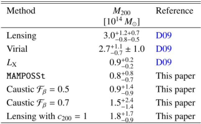
Table 4. M200estimates. Method M200 Reference [1014M ] Lensing 3.0+1.2+0.7−0.8−0.5 D09 Virial 2.7+1.1−0.7± 1.0 D09 LX 0.9+0.2−0.2 D09
MAMPOSSt 0.8+0.8−0.7 This paper
Caustic Fβ= 0.5 0.9+1.4−0.9 This paper Caustic Fβ= 0.7 1.5+2.4−1.4 This paper
Lensing with c200= 1 1.8+1.7−0.9 This paper
Notes. Statistical and systematic errors are listed (in this order) for the mass estimates ofD09.
5.2. Caustic
The Caustic method has been developed by Diaferio & Geller
(1997), andDiaferio(1999) and is a rather simple way to de-termine the mass profile of galaxy clusters from the amplitude of the galaxy velocity distribution at different distances from the cluster center. In practice, the density of galaxies in pro-jected phase-space is estimated, and then iso-density contours are defined. The iso-density contour that defines “the Caustic” is chosen by comparing the square amplitude in velocity space, weighted by the local density of galaxies, to the σv of cluster
members in the virial region. The Caustic method is supposed to work independently of the presence of substructures, and does not require the identification of cluster members, if not for the purpose of estimating the cluster σv in the virial region. Here
we determine the Caustic by using all galaxies with redshifts in the cluster region (not only members, and including galaxies in substructures), but fixing the cluster σv to the value found for
the KMM-main subcluster (see Table 2). The Caustic found is shown in Fig.5.
To convert the Caustic amplitude (along the velocity axis) into a mass estimate for the cluster, we need to choose a value for the filling factor Fβ (see Diaferio 1999, for its definition). Several values have been used so far, ranging from 0.5 to 0.7 (Diaferio & Geller 1997; Serra et al. 2011; Geller et al. 2013;
Gifford et al. 2013). Using Fβ = {0.5, 0.7} we find r200 =
0.9+0.3−0.6Mpc, and 1.0+0.4−0.6Mpc, respectively, where the uncertain-ties are evaluated following the prescriptions ofDiaferio(1999). Clearly, the statistical error dominates over the systematic uncer-tainty in the value of Fβ.
The Caustic analysis provides very poor constraints on r200
(and therefore the cluster mass), but taken at face value they are close to those obtained with MAMPOSSt (Sect.5.1) in particular for Fβ = 0.5.
6. Discussion
In Table4we list the cluster M200values found in this paper and
inD09. Both statistical and systematic errors are given for the mass estimates of D09. For the MAMPOSSt mass estimates, the listed errors include the systematics related to the unknown mass and velocity anisotropy distributions, since our choice of M(r) and β(r) models has not been restrictive. As for the Caustic mass estimates, the systematic error is dominated by the choice of Fβ,
for which we have considered the two extreme values generally adopted in the literature.
Our new kinematic estimates of M200are in agreement with
the one obtained from the cluster LXusing the scaling relation
ofRykoff et al.(2008). On the other hand, our new estimates are substantially below (by a factor of about three) the one obtained by the kinematic analysis ofD09which was based on a sample of 25 cluster members.
Numerical simulations indicate that a bias >2 is not unex-pected in kinematic mass estimates based on only ∼20 spectro-scopic members, as it occurs in 25% of the cases (Biviano et al. 2006). In these simulations, the presence of substructures along the line-of-sight was identified as the main cause of a large bias in the mass estimate (Biviano et al. 2006). While we could not identify any sign of subclustering in A315 with a sample of only 25 members, thanks to our extensive spectroscopic campaign, we have now been able to detect one small group in the external cluster regions, and, most importantly, a distinct bimodality in velocity space in the inner cluster region. This bimodality is due to two subclusters with an overlapping spatial distribution that suggests they are colliding or have collided close to the line-of-sight. The rσ200estimates of the KMM-main and KMM-sub sub-clusters imply a mass ratio of ∼0.1. Adding the KMM-sub M200
to the total cluster mass estimate therefore does not change our conclusion that our previous kinematic mass estimate of A315 has been grossly overestimated.
If the two subclusters are physically unrelated, and their ve-locity difference attributed to different Hubble flows, the smallest subcluster would lie ∼18 Mpc in the foreground. However, the subclusters are unlikely to be completely unrelated, as we can see by applying the Newtonian criterion for gravitational bind-ing of the two subclusters (Eq. (5) inBeers et al. 1991). To apply the Newtonian criterion we use the difference in the subcluster mean line-of-sight velocities (851 ± 68 km s−1), and the pro-jected separation between their centers (0.66 ± 0.10 Mpc). We use the MAMPOSSt M200estimate for the KMM-main subcluster
(see Table4) and 1/10 of this same estimate for the KMM-sub subcluster. The result is shown in Fig.10and indicates that a bound solution is acceptable within the observational uncertain-ties, for a wide range of values of the angle between the colli-sion axis and the plane of the sky. The bound solution is even more likely than our estimate indicates, because we have used M200masses, and these do not account for the additional mass
within the infall regions of the two subclusters (the total mass of the system would increase by a factor of about two;Rines et al. 2013).
The bound solution does not inform us on whether the two subclusters are observed before or after their collision. A past collision between the two subclusters might be invoked to ex-plain the very low concentration (c200 < 1) observed both
for the galaxy and the mass distribution of the main compo-nent of A315. Such a low concentration is indeed uncommon (Lin et al. 2004;Budzynski et al. 2012) and theoretically unex-pected (e.g., Correa et al. 2015c). Observationally, it has been shown that the radial distribution of galaxies in clusters with substructures is less concentrated than that of galaxies in relaxed clusters (Biviano et al. 2002). On the theoretical side, numerical simulations have shown that the scale radius of the mass distri-bution increases after a merger (Hoffman et al. 2007). A low-concentration of the mass distribution characterizes not fully virialized clusters (Jing 2000;Neto et al. 2007).
Could then the low concentration we observe originate from the collision with the subcluster identified by the KMM analy-sis? To answer this question, we estimate the probability of a halo of mass similar to the mass of A315, to have a concentra-tion c200 < 2.9. This is the highest value that is still marginally
Fig. 10.The black line shows the requirement for the two KMM sub-clusters to be gravitationally bound, as computed from the Newtonian criterion; the grey shading indicates 1σ uncertainties on this require-ment, which depends on the projected distance and line-of-sight veloc-ity difference of the two subclusters. The red line indicates the sum of the measured masses for these subclusters; the orange shading indicates 1σ uncertainties on this sum. On the x-axis, the angle between the axis connecting the KMM-main and KMM-sub subclusters is defined with respect to the plane of the sky (90 degrees corresponds to a line-of-sight collision). The KMM subclusters are gravitationally bound for an angle between ∼35 and ∼75 degrees, if we take into account both the uncertainties on our mass estimates and the uncertainties on the Newton criterion requirements.
acceptable according to our MAMPOSSt dynamical analysis of A315 (dotted curve in Fig,9). We use the concentration distri-butions of the halos in the Millennium Simulation derived by
Neto et al. (2007). More precisely, we consider the lognormal best-fit models listed in their Table 1, for the halos in the mass range closest to our A315 mass estimate. While only 1% of re-laxed halos have c200 < 2.9, 28% of unrelaxed halos have such
a low concentration or lower. This fraction drops to 0.005% at c200< 1. It then appears that the best-fit concentration value we
observe is rarely observed in cosmological simulated halos, but not when we account for the observational uncertainties and for the unrelaxed nature of A315.
The low-concentration of the mass distribution of A315 might also account for part of the mass overestimate from lensing (D09).D09 treated the NFW profile as a 1-parameter profile where the concentration follows the theoretical mass-concentration relation ofDolag et al.(2004) exactly. At the best fit M200 inD09the concentration used was 7.0. Performing a
two-parameter fit, with a free concentration parameter is un-fortunately not allowed by the quality of theD09data. In par-ticular, the low total number of galaxies inside the NFW scale radius limits the constraining power of this data set. Further-more, contamination of the catalog of lensed galaxies by clus-ter galaxies dilutes the shear signal in a radially-dependent way that is extremely challenging to model even for much better quality data than those of D09. We therefore repeat the weak lensing analysis of D09 on the same data and with the same technique, but this time forcing c200 = 1 instead. We obtain
M200= 1.8+1.7−0.9× 10¹⁴ M , that brings the lensing mass estimate
in agreement with the kinematic and X-ray estimates within 1σ (see Fig.9and Table4).
In addition, the lensing mass estimate might be further re-duced by considering that it is derived assuming a spherical NFW profile, while the cluster mass distribution is elongated
along the line-of-sight due to the two overlapping subclusters (e.g.,Corless & King 2007;Dietrich et al. 2014). If the elonga-tion is only due to the superposielonga-tion of the two subclusters, we expect the effective axis ratio of the total mass distribution not to be too far from unity. However, in low concentration clusters, the mass ratio between the best-fitting lensing mass obtained as-suming a spherical NFW halo and the true mass of an elliptical NFW halo, can be ∼1.1 also for a relatively small axis ratio (see Fig. 2 inDietrich et al. 2014).
Due to its dependence on the square of the electron density, X-ray luminosity-based mass estimates are to a good approxi-mation not affected by triaxiality. However, the low mass con-centration suggests that A315 might be a non-cool-core cluster. The mass estimate that one obtains from LXvia a scaling relation
obtained for an unbiased cluster sample, is systematically lower for non-cool-core clusters, by ∼25% (see Fig. 3 inZhang et al. 2011). Indeed, scaling relations with core-excised LXhave less
dispersion and lower systematics than those obtained from the total LX(Mittal et al. 2011).
The presence of substructure in the velocity distribution of A315 and its low mass concentration, thus seems to be able to reconcile the X-ray, lensing, and kinematic cluster mass es-timates. Possibly the presence of substructures and the low mass concentration are both the manifestation of the same phe-nomenon, namely a collision along the line-of-sight of a poor cluster and a galaxy group.
In conclusion, our new analysis rules out the X-ray underlu-minous nature of A315, just as it was done for A1456 byD09. These clusters appear X-ray underluminous because their veloc-ity dispersions are inflated by infalling, unrelaxed halos – an in-terpretation originally given by Bower et al. (1997) to explain the existence of low-LXclusters with high σv.
A315 and A1456 are however only 2 of 51 AXU clusters in the sample ofP07. Both were found to be characterized by a bimodal velocity distribution when analyzed in detail and with more spectroscopic data (in the case of A315). Such a velocity distribution is characterized by low T I values (like the one we obtain for the Inner sample of A315, see Table2), as expected from the presence of two kinematically distinct components with a mean velocity offset (see, e.g., the case of A85 in the study ofBeers et al. 1991). However, low T I values are not typical of AXU clusters, thatP07found instead to have velocity distribu-tions characterized by high T I values outside the virial region, a feature that remains to be explained. One possibility is that high T I values are caused by the presence of high-velocity interlop-ers that are not removed by the membinterlop-ership selection procedure, which could fail for poor statistical samples. More detailed in-vestigations of other AXU clusters are needed before we can dis-miss the existence of intrinsically X-ray underluminous clusters altogether.
7. Conclusions
We re-determine the kinematic mass estimate of the z = 0.174 cluster A315, which had previously been identified as being X-ray underluminous for its kinematic and lensing mass (P07;
D09). Our new kinematic estimate is based on redshifts for ∼200 cluster members, in part obtained through our new spec-troscopic observations with VIMOS at the VLT. These are the results of our analysis:
– We identify previously undetected substructures. In particu-lar, the velocity distribution of cluster members in the virial
region displays a significant bimodality, caused by the pro-jection of two distinct subclusters along the line-of-sight. – Accounting for these substructures in our kinematic
anal-ysis (conducted via MAMPOSSt and the Caustic method,
Mamon et al. 2013; Diaferio & Geller 1997, respectively), leads to a substantial and significant reduction of the kine-matic mass estimate ofD09, which was based on 25 mem-bers only. Our kinematic mass estimate, 0.8+0.6−0.4× 10¹⁴M , is
in agreement with the estimate that we obtain from the clus-ter LX through the scaling relation ofRykoff et al.(2008),
0.9 ± 0.2 × 10¹⁴ M .
– In our dynamical analysis we also determine the cluster mass concentration. We find c200< 1, an unusually low value. We
argue that this is the effect of a ∼1:10 mass-ratio collision between the two subclusters identified in the virial region. – Using our estimate of c200, we redetermine the weak
lens-ing mass of A315 uslens-ing the same method of D09, and we find M200 = 1.8+1.7−0.9M . This mass estimate is 40%
lower than the estimate of D09, which was obtained us-ing a much higher concentration, inferred from a theoreti-cal concentration-mass relation. Accounting for elongation of the cluster along the line-of-sight could further reduce our new lensing mass estimate (by&10%).
– The low-mass concentration we find might suggest that A315 is not a cool-core cluster. Its LXmight therefore correspond
to a slightly higher mass (by ∼25%) than the one predicted by theRykoff et al.(2008) scaling relation.
Our new results dismiss the AXU nature of A315, just as it was done for A1456 byD09. The A315 LXno longer appears too low
for its mass. Its lensing mass had been over-estimated because it was derived assuming a normal mass concentration, rather than the true, very small one. The cluster kinematic mass had previ-ously been over-estimated because of an undetected bimodality in its velocity distributions. This was also the case of A1456. Both clusters belong to the category of systems whose velocity dispersions are inflated by infalling subclusters or groups pro-jected along the line-of-sight (Bower et al. 1997). Whether line-of-sight projections are the only explanation for the nature of AXU clusters is impossible to say before more candidates are examined with the same level of detail used for A315. These studies will help quantifying the biases in cluster mass estimates, a fundamental issue for the use of clusters as cosmological probes.
Acknowledgements. We dedicate this work to the memory of our friend and col-league Yu-Yin Zhang, whose collaboration we have enjoyed and appreciated for several years. We thank the anonynous referee for her/his useful comments. A.B. acknowledges the hospitality of the Excellence Cluster Universe, and financial support provided by the PRIN INAF 2014: “Glittering kaleidoscopes in the sky: the multifaceted nature and role of Galaxy Clusters”, P.I.: Mario Nonino. Y.Y.Z. acknowledges support by the German BMWi through the Verbundforschung un-der grant 50 OR 1304. This paper has made use of data from SDSS-III. Funding for SDSS-III has been provided by the Alfred P. Sloan Foundation, the Partici-pating Institutions, the National Science Foundation, and the US Department of Energy Office of Science. The SDSS-III web site ishttp://www.sdss3.org/. SDSS-III is managed by the Astrophysical Research Consortium for the Par-ticipating Institutions of the SDSS-III Collaboration including the University of Arizona, the Brazilian Participation Group, Brookhaven National Labora-tory, Carnegie Mellon University, University of Florida, the French Participation Group, the German Participation Group, Harvard University, the Instituto de As-trofisica de Canarias, the Michigan State/Notre Dame/JINA Participation Group, Johns Hopkins University, Lawrence Berkeley National Laboratory, Max Planck Institute for Astrophysics, Max Planck Institute for Extraterrestrial Physics, New Mexico State University, New York University, Ohio State University, Penn-sylvania State University, University of Portsmouth, Princeton University, the Spanish Participation Group, University of Tokyo, University of Utah, Van-derbilt University, University of Virginia, University of Washington, and Yale University.
References
Arnaud, M., Pointecouteau, E., & Pratt, G. W. 2005,A&A, 441, 893
Ashman, K. M., Bird, C. M., & Zepf, S. E. 1994,AJ, 108, 2348
Bartelmann, M. 1996,A&A, 313, 697
Basilakos, S., Plionis, M., Georgakakis, A., et al. 2004,MNRAS, 351, 989
Beers, T. C., Flynn, K., & Gebhardt, K. 1990,AJ, 100, 32
Beers, T. C., Gebhardt, K., Forman, W., Huchra, J. P., & Jones, C. 1991,AJ, 102, 1581
Bhattacharya, S., Habib, S., Heitmann, K., & Vikhlinin, A. 2013,ApJ, 766, 32
Bird, C. M., & Beers, T. C. 1993,AJ, 105, 1596
Biviano, A. 2008, ArXiv e-prints [arXiv:0811.3535] Biviano, A., & Katgert, P. 2004,A&A, 424, 779
Biviano, A., & Poggianti, B. M. 2009,A&A, 501, 419
Biviano, A., Durret, F., Gerbal, D., et al. 1996,A&A, 311, 95
Biviano, A., Katgert, P., Thomas, T., & Adami, C. 2002,A&A, 387, 8
Biviano, A., Murante, G., Borgani, S., et al. 2006,A&A, 456, 23
Biviano, A., Rosati, P., Balestra, I., et al. 2013,A&A, 558, A1
Boschin, W., Barrena, R., Girardi, M., & Spolaor, M. 2008,A&A, 487, 33
Bower, R. G., Castander, F. J., Ellis, R. S., Couch, W. J., & Boehringer, H. 1997,
MNRAS, 291, 353
Budzynski, J. M., Koposov, S. E., McCarthy, I. G., McGee, S. L., & Belokurov, V. 2012,MNRAS, 423, 104
Burkert, A. 1995,ApJ, 447, L25
Burns, J. O., Hallman, E. J., Gantner, B., Motl, P. M., & Norman, M. L. 2008,
ApJ, 675, 1125
Corless, V. L., & King, L. J. 2007,MNRAS, 380, 149
Correa, C. A., Wyithe, J. S. B., Schaye, J., & Duffy, A. R. 2015a,MNRAS, 450, 1514
Correa, C. A., Wyithe, J. S. B., Schaye, J., & Duffy, A. R. 2015b,MNRAS, 450, 1521
Correa, C. A., Wyithe, J. S. B., Schaye, J., & Duffy, A. R. 2015c,MNRAS, 452, 1217
De Boni, C., Ettori, S., Dolag, K., & Moscardini, L. 2013,MNRAS, 428, 2921
Diaferio, A. 1999,MNRAS, 309, 610
Diaferio, A., & Geller, M. J. 1997,ApJ, 481, 633
Dietrich, J. P., Biviano, A., Popesso, P., et al. 2009,A&A, 499, 669
Dietrich, J. P., Zhang, Y., Song, J., et al. 2014,MNRAS, 443, 1713
Dolag, K., Bartelmann, M., Perrotta, F., et al. 2004,A&A, 416, 853
Donahue, M., Scharf, C. A., Mack, J., et al. 2002,ApJ, 569, 689
Dressler, A., & Shectman, S. A. 1988,AJ, 95, 985
Eckert, D., Molendi, S., & Paltani, S. 2011,A&A, 526, A79
Efron, B., & Tibshirani, R. 1986,Stat. Sci., 1, 54
Eisenstein, D. J., Weinberg, D. H., Agol, E., et al. 2011,AJ, 142, 72
Fadda, D., Girardi, M., Giuricin, G., Mardirossian, F., & Mezzetti, M. 1996,ApJ, 473, 670
Freudling, W., Romaniello, M., Bramich, D. M., et al. 2013,A&A, 559, A96
Geller, M. J., Diaferio, A., Rines, K. J., & Serra, A. L. 2013,ApJ, 764, 58
Gifford, D., Miller, C., & Kern, N. 2013,ApJ, 773, 116
Gilbank, D. G., Bower, R. G., Castander, F. J., & Ziegler, B. L. 2004,MNRAS, 348, 551
Giocoli, C., Meneghetti, M., Metcalf, R. B., Ettori, S., & Moscardini, L. 2014,
MNRAS, 440, 1899
Girardi, M., Biviano, A., Giuricin, G., Mardirossian, F., & Mezzetti, M. 1993,
ApJ, 404, 38
Guennou, L., Biviano, A., Adami, C., et al. 2014,A&A, 566, A149
Hernquist, L. 1990,ApJ, 356, 359
Hoekstra, H., Herbonnet, R., Muzzin, A., et al. 2015,MNRAS, 449, 685
Hoffman, Y., Romano-Díaz, E., Shlosman, I., & Heller, C. 2007,ApJ, 671, 1108
Israel, H., Reiprich, T. H., Erben, T., et al. 2014,A&A, 564, A129
Jing, Y. P. 2000,ApJ, 535, 30
Johnston, D. E., Sheldon, E. S., Tasitsiomi, A., et al. 2007,ApJ, 656, 27
Knobel, C., Lilly, S. J., Iovino, A., et al. 2009,ApJ, 697, 1842
Kravtsov, A. V., & Borgani, S. 2012,ARA&A, 50, 353
Kurtz, M. J., & Mink, D. J. 1998,PASP, 110, 934
Le Fèvre, O., Saisse, M., Mancini, D., et al. 2003, in SPIE Conf. Ser., 4841, eds. M. Iye, & A. F. M. Moorwood, 1670
Lin, Y.-T., Mohr, J. J., & Stanford, S. A. 2004,ApJ, 610, 745
Macciò, A. V., Dutton, A. A., & van den Bosch, F. C. 2008,MNRAS, 391, 1940
Mamon, G. A., & Łokas, E. L. 2005,MNRAS, 363, 705
Mamon, G. A., Biviano, A., & Boué, G. 2013,MNRAS, 429, 3079
Markevitch, M., Gonzalez, A. H., David, L., et al. 2002,ApJ, 567, L27
McLachlan, G. J., & Basford, K. E. 1988, Mixture Models: Inference and Applications to Clustering (New York: Marcel Dekker)
Merritt, D. 1985,ApJ, 289, 18
Mittal, R., Hicks, A., Reiprich, T. H., & Jaritz, V. 2011,A&A, 532, A133
Montero-Dorta, A. D., & Prada, F. 2009,MNRAS, 399, 1106
Munari, E., Biviano, A., Borgani, S., Murante, G., & Fabjan, D. 2013,MNRAS, 430, 2638
Munari, E., Biviano, A., & Mamon, G. A. 2014,A&A, 566, A68
Navarro, J. F., Frenk, C. S., & White, S. D. M. 1997,ApJ, 490, 493
Neto, A. F., Gao, L., Bett, P., et al. 2007,MNRAS, 381, 1450
Ntampaka, M., Trac, H., Sutherland, D. J., et al. 2015,ApJ, 803, 50
Osipkov, L. P. 1979,Sov. Astron. Lett., 5, 42
Planck Collaboration XX. 2014,A&A, 571, A20
Polletta, M., Tajer, M., Maraschi, L., et al. 2007,ApJ, 663, 81
Poole, G. B., Babul, A., McCarthy, I. G., Sanderson, A. J. R., & Fardal, M. A. 2008,MNRAS, 391, 1163
Popesso, P., Biviano, A., Böhringer, H., Romaniello, M., & Voges, W. 2005,
A&A, 433, 431
Popesso, P., Biviano, A., Böhringer, H., & Romaniello, M. 2007,A&A, 461, 397, (P07)
Ramella, M., Zamorani, G., Zucca, E., et al. 1999,A&A, 342, 1
Rasia, E., Ettori, S., Moscardini, L., et al. 2006,MNRAS, 369, 2013
Rines, K., Geller, M. J., Diaferio, A., & Kurtz, M. J. 2013,ApJ, 767, 15
Roettiger, K., Burns, J. O., & Loken, C. 1996,ApJ, 473, 651
Ross, A. J., Samushia, L., Burden, A., et al. 2014,MNRAS, 437, 1109
Rozo, E., Rykoff, E. S., Bartlett, J. G., & Melin, J.-B. 2015,MNRAS, 450, 592
Rykoff, E. S., Evrard, A. E., McKay, T. A., et al. 2008,MNRAS, 387, L28
Sadibekova, T., Pierre, M., Clerc, N., et al. 2014,A&A, 571, A87
Sartoris, B., Borgani, S., Rosati, P., & Weller, J. 2012,MNRAS, 423, 2503
Sartoris, B., Biviano, A., Fedeli, C., et al. 2016,MNRAS, 459, 1764
Sereno, M., Ettori, S., & Moscardini, L. 2015,MNRAS, 450, 3649
Serra, A. L., Diaferio, A., Murante, G., & Borgani, S. 2011,MNRAS, 412, 800
Smith, G. P., Mazzotta, P., Okabe, N., et al. 2016,MNRAS, 456, L74
Umetsu, K., Medezinski, E., Nonino, M., et al. 2012,ApJ, 755, 56
Umetsu, K., Medezinski, E., Nonino, M., et al. 2014,ApJ, 795, 163
von der Linden, A., Mantz, A., Allen, S. W., et al. 2014,MNRAS, 443, 1973
Wojtak, R., & Łokas, E. L. 2010,MNRAS, 408, 2442
Zhang, Y.-Y., Andernach, H., Caretta, C. A., et al. 2011,A&A, 526, A105
Zhang, C., Yu, Q., & Lu, Y. 2014,ApJ, 796, 138
Appendix A: The modified Dressler and Shectman (DSb) test
The original version of the test looked for these deviations in all possible groups of 11 neighboring galaxies identified within a cluster (Dressler & Shectman 1988).Biviano et al.(1996, see Appendix A.3 in that paper) adapted this method to make adaptive-kernel maps of the quantity δ that describes the aver-age velocity and velocity dispersion deviation from the global cluster value.Biviano et al.(2002) then modified δ into its two components δv and δσ, that separately measure the local devi-ations of the average velocity and velocity dispersion, respec-tively. They also introduced the use of the velocity dispersion profile, in lieu of the total cluster velocity dispersion, as a refer-ence value for δσ.
Fig. A.1.Cluster projected velocity dispersion profile, normalized by the total velocity dispersion (dots with 1σ error bars). The solid curve represent the smoothed profile, adopted in the Dressler and Shectman test. The dashed curve shows, for comparison, the smoothed profile ob-tained for a sample of nearby clusters byBiviano et al.(2002).
We combine the modifications proposed by Biviano et al.
(1996; and2002). Specifically, we evaluate the local values of mean velocity and velocity dispersion by constructing weighted adaptive-kernel density maps of cluster members, with the weights given by v and v2, and dividing these maps by the un-weighted adaptive-kernel number density map of cluster mem-bers, δv(x)= N X j=1 K(2D)j (x)vj/ N X j=1 K(2D)j (x) (A.1) δσ(x)= N X j=1 K(2D)j (x)v2j/ N X j=1 K(2D)j (x) 1/2 −σv(R) (A.2)
where K(2D)j (x) is the 2D kernel at the position x, and σv(R) is the total cluster velocity dispersion profile, that is the velocity dispersion at a given projected position R, shown in Fig.A.1.
The significance of the δvand δσ at any position x are eval-uated separately, by bootstrap resamplings (Efron & Tibshirani 1986).