In this thesis, I designed and implemented three new web applications tai-lored for the Cellular Automata (CA) simulation models SCIDDICA-k1, SCIARA-fv3 and ABBAMPAU, making use of the Google Web Toolkit frame-work and WebGL.
Moreover, I have contributed to the optimizations of the numerical models mentioned above and I also developed part of a library, called OpenCAL, for developing CA simulation models in C/C++. In this case, my most signifi-cant contribution regarded the support given to the parallelization through the OpenCL standard, in order to facilitate with a few lines of codes, the par-allelization for the execution on any device, especially on General Purpose Computation with Graphics Processing Units (GPGPU).
The development of the web applications involved the implementation of strategies so that optimizing the server load in the connections’ management and enhancing the real time visualization of maps on devices of any kind, even mobile.
As regards the OpenCAL library, the tests performed on a test models has shown significant performance improvements in terms of speedup, thanks also to the use of some new optimization strategies. In this way, the validity of the use of graphics processing units as alternative to more expensive hardware solutions for the parallelization of CA models has been confirmed.
In questo lavoro di tesi ho progettato e implementato tre web application per i modelli di simulazione ad Automi Cellulari SCIDDICA-k1, SCIARA-fv3 e ABBAMPAU, utilizzando il framework Google Web Toolkit e WebGL.
Inoltre, ho contribuito ad alcune ottimizzazioni dei modelli numerici so-pra citati e ho sviluppato parte di una libreria, chiamata OpenCAL, per lo sviluppo di modelli di simulazione ad Automi Cellulari in C/C++. Il mio contributo pi´u significativo ha riguardato la parallelizzazione della libreria in OpenCL per consentire una parallelizzazione semplificata dell’automa cellu-lare rispetto all’impoego diretto di OpenCL e l’esecuzione su device etero-genei, in particolar modo su schede grafiche per il calcolo general-purpose (General Purpose Computation with Graphics Processing Units - GPGPU). Lo sviluppo delle web application ha coinvolto l’applicazione di strate-gie per ottimizzare il carico dei server nella gestione delle connessioni e per rendere pi´u performante la visualizzazione in tempo reale delle mappe su qualsiasi tipo di dispositivo, anche mobile.
Per quanto riguarda la libreria OpenCAL, gli esperimenti effettuati su al-cuni modelli base mostrano significativi miglioramenti nelle performance in termini di speedup, grazie anche all’utilizzo di alcune strategie d’ottimizzazio-ne nuove, confermando la validit´a dell’uso di processori grafici come alterna-tiva a soluzioni hardware classiche, generalemente piu‘ costose, per la paral-lelizzazione di modelli ad Automi Cellulari.
1 Introduction 1
2 A brief overview of Cellular Automata, GPGPU and Web
2.0 4
2.1 Cellular Automata . . . 4
2.1.1 Informal Definition . . . 6
2.1.1.1 Cellular space dimension and geometry . . . . 6
2.1.1.2 Neighborhood . . . 7
2.1.1.3 Transition Function . . . 8
2.1.2 Formal Definition . . . 8
2.1.2.1 Finite State Automaton . . . 8
2.1.3 Homogeneous Cellular Automata . . . 10
2.1.4 Theories and studies . . . 12
2.1.4.1 Elementary cellular automata . . . 12
2.1.4.2 Wolfram’s classification . . . 13
2.1.4.3 At the edge of Chaos . . . 14
2.1.4.4 Game of life . . . 17
2.1.5 Extension of the Cellular automata model . . . 19
2.1.5.1 Probabilistic CA . . . 19
2.2 GPGPU Technologies . . . 21
2.2.1 Why GPU computing? . . . 21
2.2.2 From Graphics to General Purpose Computing . . . 23
2.2.2.1 Traditional Graphics Pipeline . . . 24
2.2.3 CUDA . . . 27
2.2.3.1 CUDA Programming model . . . 28
2.2.3.2 CUDA Threads and Kernels . . . 29
2.2.3.3 Memory hierarchy . . . 31
2.2.3.4 Programming with CUDA C . . . 32
2.2.4 OpenCL . . . 33
2.2.4.1 Model Architecture . . . 33
2.2.5 OpenACC . . . 37
2.2.5.1 Wait Directive . . . 39
2.2.5.2 Kernel Directive . . . 39
2.2.5.3 Data Construct . . . 39
2.3 WEB 2.0 . . . 39
2.3.1 The dawn of the Web . . . 40
2.3.2 The Web 2.0 . . . 43
2.4 AJAX . . . 44
2.4.1 AJAX rich applications . . . 46
2.4.1.1 Benefits and Drawbacks . . . 48
3 Simulation of complex macroscopic natural phenomena and Scientific Web applications 52 3.1 Cellular Automata application Models . . . 52
3.1.1 SCIDDICA K1: a cellular automata model to simulate landslides and debris flows. . . 52
3.1.1.1 Applications of the model SCIDDICA K1. . . 59
3.1.2 SCIARA-fv3 - Model Formalization . . . 63
3.1.2.1 Model Overview . . . 63
3.1.2.2 Elementary process . . . 64
3.1.3 ABBAMPAU a CA for Wildfire Simulation and Risk Assessment . . . 71
3.2 Web applications . . . 76
3.2.1 Swii2 . . . 77
3.2.1.1 The system architecture . . . 77
3.2.1.2 The Swii2 GUI and the visualization system . 79 3.2.1.3 Swii2 preliminary analysis . . . 80
3.2.1.4 Cooperative Aspects in Scientific Simulation . 80 3.2.2 SciaraWii: the SCIARA-fv3 Web User Interface . . . . 82
3.2.2.1 System architecture . . . 82
3.2.2.2 Visualization system, Rendering And Deci-mation . . . 82 3.2.2.3 Performance analysis . . . 83 3.2.3 Awii . . . 84 3.2.3.1 System architecture . . . 85 3.2.3.2 Performance analysis . . . 87 4 OpenCAL 88 4.1 A brief description of OpenCAL . . . 89
4.1.1 An OpenCAL implementation of Conway’s Game of Life 89 4.1.2 An OpenCAL implementation of the SCIDDICA-T de-bris flows model . . . 94
4.2 A brief description of the OpenCAL parallel OpenCL version . 101 4.2.1 OpenCAL improvement to OpenCL programming . . . 102 4.2.2 A simple OpenCAL parallel example of application:
The Game of Life . . . 107 4.2.3 A more complex OpenCAL parallel example of
appli-cation: SCIDDICA-T . . . 110 4.3 OpenCAL parallel computational performance . . . 116
5 Conclusions 120
Acknowledgments 123
Bibliography 124
List of Figures 131
1
Introduction
From the early days of Computer Science, one of the most important purposes of computers was the simulation of the natural phenomena. With these simulations, man has the total control of the reproduced “world” [37] and he can test his theories and assumptions by comparing it to the reality. Indeed, the execution speed of computers has allowed the use of numerical simulation as an instrument to solve complex equations systems, with which scientists can “model” the complex phenomena of reality. Nowadays, these simulations gain a particular importance because they are not only used to test theories and assumptions, but also to prevent, in medium and long-term, the evolution over time of a complex system; in this context the prevention of natural disasters, weather forecasts, evaluations of financial trends and so on are placed. The application fields of simulations are countless; for example, they can be used for the vocational education of those professionals for which the training in a real environment would lead to safety problems or costs (such as in pilots’ training).
However, many real systems are not suitable for an immediate and natu-ral “classical” modeling, based on a first analytical and deductive phase, fol-lowed by a later resolution through numerical methods. In complex systems’ simulation the computational paradigm of Cellular Automata [71] is widely adopted, which represent, in some contexts, an alternative method to sys-tems in which are used differential equations, especially employed in Physics to describe the laws that rule the evolution of a phenomenon. According to the Cellular Automata modeling approach, a system can be considered as
composed of several simple elements, each one evolves following purely local laws. The global evolution of the system then “emerges” from the evolution of all constituent elements. Cellular Automata are successfully used to sim-ulate complex systems in several fields, like Computational Fluid Dynamics, Artificial Life, Molecular Dynamics, Biology, Genetics, Chemistry, Geology, Cryptography, Financial world,Territorial Analysis, modeling of road traffics, image processing.
In the execution of the simulations it is often necessary to perform a considerable quantity of computations. It may then happen that, in some contexts, computers take excessively long processing times, making the simu-lations useless for practical purposes. For this reason, it is required to speed up the simulations; therefore, it is useful to resort on parallel computers, composed by many processing units able to run many programs simultane-ously, in order to solve different problems or execute a single problem taking less time.
However, the use of high-performance parallel computers (supercomput-ers) is not always possible for who needs to simulate complex phenomena such as certain geological phenomena that are of particular interest in order to prevent disasters. In Italy, for example, it would be desirable to be able to simulate in advance the effects of landslides that could hit the territory, which is particularly exposed to this kind of phenomena.
Usually, softwares allow an interactive simulation and integrate a 2D and/or 3D visualization system. In most cases, however it is sequential soft-ware, despite the current technological development can permit to have access to parallel systems with high computational capacity at low cost (compared to the past). This is true especially in the case of General-Purpose Compu-tation with Graphics Processing Units (GPGPU), which uses the graphics cards for computational purposes. Generally, for Desktop Applications com-putation and visualization are combined in a single software. In some cases, however, it is possible to find examples of client-server applications where the computational part is independent from the graphical interface and the visualization system; the computation can therefore be performed remotely, possibly on supercomputers. A further development is given by the most recent Web technologies, thanks to which it is possible to realize on one hand graphical interfaces comparable, if not better, to classical ones, and on the other hand complete and functional interactive systems for 2D and 3D scientific visualization. Furthermore, web applications improve the level of usability of the applications itself and remove those problems related to soft-ware download. Besides, the end user does not have to worry about where the computation is executed, nor the details of the computational model used.
supercomputing and Web 2.0 converge in order to realize new applications for computational models for the simulation of complex systems. For this purpose, three Cellular Automata numerical models and three respective web applications have been implemented, each one with an interactive 3D visualization system, implemented using WebGL. The implemented models are: SCIDDICA-k1 with the Swii2 web application for debris flows simula-tion, SCIARA-fv3 with SciaraWii for lava flows and ABBAMPAU with Awii to display and control the evolution of wildfire. Instead, as regards the as-pects related to the increase of performance, a significant contribution to the development of a new library for Cellular Automata has been carried out, especially to its parallelization in OpenCL for the execution on GPUs.
The thesis is organized as described below. The second Chapter focuses on different theoretical arguments and the presentation of some simulation models: the Cellular Automata with their most important theoretical results and some common applications; their specifically application for modelling and simulating some natural complex phenomena; the algorithm for the min-imisation of differences [19]; there is also an overview on GPGPU techniques like CUDA, OpenCL and OpenACC; a general description of the innovations introduced by the WEB 2.0; finally, the AJAX development method, its applications and the resultant innovative effects. The third Chapter shows our latest release on lava flows simulations, debris flow simulations and wild-fire simulations, SCIARA-fv3, SCIDDICA-k1 and ABBAMPAU, respectively and the structures of SCIDDICA, SCIARA and ABBAMPAU Web Interac-tive Interfaces are described, with some applications and the main differences among them. Software architecture is described, as well as the 3D visualiza-tions systems based on WebGL. The fourth Chapter focuses on the descrip-tion of the OpenCAL library and the advantages by using its OpenCL sup-port. Then, some implementations and performance analysis are reported. The last Chapter concludes with general discussions and directions for future work.
2
A brief overview of Cellular Automata,
GPGPU and Web 2.0
2.1
Cellular Automata
Nowadays most of natural phenomena are well described and known, thanks to the effort of scientists that studied the basic physic’s laws for centuries; for example, the freezing of water or the conduction that are well know and qualitative analyzed. Natural systems are usually composed by many parts that interact in a complex net of causes/consequences that is at least very difficult but most of the times impossible to track and to describe. Even if the single components are each very simple, extremely complex behavior emerge naturally due to the cooperative effect of many components. Much has been discovered about the nature of the components in natural systems, but lit-tle is known about the interactions that these components have in order to give the overall complexity observed. Classical theoretical investigations of physical system have been based on mathematical models, like differential equations, that use calculus as tool to solve them, which are able to describe and allow to understand the phenomena, in particular for those that can be described by which are linear differential equation1 that are easy solvable with calculus. Problems arise when non-linear differential equations come
1Some electro-magnetism phenomena, for instance, can be described by linear
differ-ential equations.
out from the modellation of the phenomena, like fluid turbulence2. Classical approaches usually fails to handle these kind of equations due to the elevated number of components, that make the problem intractable even for a com-puter based numerical approach. Another approach to describe such systems is to distill only the fundamental and essential mathematical mechanism that yield to the complex behavior and at the same time capture the essence of each component process.
Figure 2.1: A 3D cellular automaton with toroidal cellular space. Cellular Automata (CA) are a candidate class of such systems and are well suitable for the modellation and simulation of a wide class of systems, in particular those ones constructed from many identical components, each (ideally) simple, but together capable of complex behaviour [65] [66]. In liter-ature there are lots applications of Cellular Automata in a wide rage of class problems from gas [25] and fluid turbulence [62] simulation to macroscopic phenomena [30] like epidemic spread [59], snowflakes and lava flow [15] [60]. CA were first investigated by S. Ulam working on growth of crystals using lattice network and at the same time by Von Neumann in order to study self-reproduction [70]; it was not very popular until the 1970 and the famous Conway’s game of life [13], then was widely studied on the theoretical view-point, computational universality were proved3[64] and then mainly utilised, after 1980’s, as a parallel model due to its intrinsically parallel nature imple-mented on parallel computers [46].
2Conventionally described by Navier-Stokes differential equations.
3CA is capable of simulating a Turing machine, i.e. is capable of computing every
computable problems (Church-Turing thesis). For instance, Game of life was proved to be capable of simulating logical gates (with special patterns as gliders and guns).
2.1.1
Informal Definition
Informally, a cellular automaton is a mathematical model that consists of a discrete lattice of sites and a value, the state, that is updated in a sequence of discrete timestamps (steps) according to some logical rules that depend on a neighbor sites of the cell. Hence CA describe systems whose the overall behavior and evolution of the system may be exclusively described on the basis of local interactions [75]. The most stringent and typical characteristic of the CA-model is the restriction that the local function does not depend on the time t or the place i: a cellular automaton has homogeneous space/time behavior. It is for this reason that CA are sometimes referred to as shift-dynamical or translation invariant systems. From another point of view we can say that in each lattice site resides a finite state automaton4 that take as input only the states of the cells in its neighborhood (see figure 2.4). 2.1.1.1 Cellular space dimension and geometry
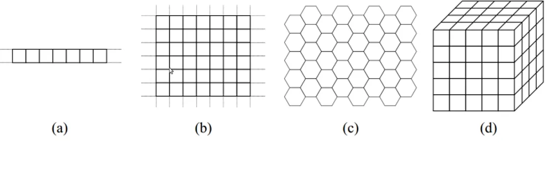
The cellular space is a discrete d-dimensional lattice of sites (see figure 2.2). For 1-D automaton the only way to discretize the space is in a one-dimensional grid. For automaton with one-dimensionality higher than 1 the shape of each cell can be different than squared. In 2D tessellation for example each cell can be hexagonal or triangular instead of squared. Each tessella-tion present advantages and disadvantages. For instance the squared one does not give any graphical representation problem5, but present problems of anisotropy for some kind of simulations6 [25]. An hexagonal tessellation can solve the anisotropy problem [73] but presents obvious graphical issues. Often, to avoid complications due to a boundary, periodic boundary condi-tions are used, so that a two-dimensional grid is the surface of a torus (see picture 2.1).
4A simple and well know computational model. It has inputs, outputs and a finite
number of states (hence a finite amount of memory); An automata changes state at regular time-steps.
5Each cell could be easily mapped onto a pixel.
6The HPP model for fluid simulation was highly anisotropic due to the squared
Figure 2.2: Examples of cellular spaces. (a) 1-D, (b) 2-D squared cells, (c) 2-D hexagonal cells, (d) 3-D cubic cells.
2.1.1.2 Neighborhood
The evolution of a cell’s state is function of the states of the neighborhood’s cells. The geometry and the number of cells that are part of the neighbor-hood depends on the tessellation type, but it has to have three fundamental properties:
1. Locality. It should involve only a “limited” number of cells. 2. Invariance. It should not be changed during the evolution.
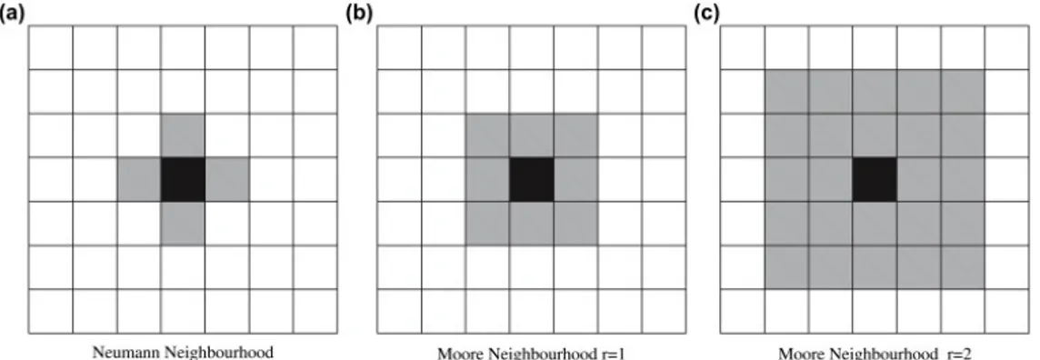
3. Homogeneity. It has to be the same for each cell of the automaton. Typically neighborhood “surrounds” the central cell. For 1-D cellular au-tomata its borders are identified with a number r called radius [74]. A r = 2 identify n = 2r + 1 cells in a 1D lattice: the central cell plus the right and left cells. Typical 2D cellular space neighborhood are the those of Moore and von Neumann neighborhood. The number of cells in the Moore neighborhood of range r is the odd squares (2r + 1)2, the first few of which are 1, 9, 25, 49, 81, and so on as r is increased. Von Neumann’s one consist of the central cell plus the cell at north, south, east, and west of the central cell itself. Moore’s (r = 1) one add the farther cells at north-east, south-east, south-west and north-west (see figure 2.3).
Figure 2.3: Examples of different kind of neighborhood with different radius values.
2.1.1.3 Transition Function
The evolution of the cell’s state is decided by the transition function that is applied at the same time and on each cell. Usually the transition function is deterministic and defined by a look-up table only when the total number of state for each cell is small7 otherwise is defined by an algorithmic procedure. It may be probabilistic, in the case of stochastic cellular automata.
2.1.2
Formal Definition
Cellular automata are dynamic models that are discrete in time, space and state. A simple cellular automaton A is defined by a lattice of cells each containing a finite state automaton, so we briefly give its definition.
2.1.2.1 Finite State Automaton
Also known as deterministic finite automata (DFAs) or as deterministic finite state machines, ther are one of the most studied and simple known compu-tational models . It is a theoretical model of computation8 that can be in a finite number of states, only one at a time, the current state. Its state can change in response of inputs taken by a transition function that describe the state change given the current state and the received input of the automata. They are much more restrictive in their capabilities than a Turing machines 9, but they are still capable to solve simpler problems, and hence to
recog-7Otherwise the dimension of that table would be enormous because the number of
entries is exponential in the number of states.
8Language recognition problem solvers.
9For example we can show that is not possible for an automaton to determine whether
nize simpler languages, like well parenthesized string; More in general they are capable to recognize the so called Regular languages10, but they fail for example in parsing context-free languages. More formally a DFA is a 5-tuple:
M =< Q, Σ, δ, q0, F > • Q is a finite, nonempty, set of states. • Σ is the alphabet
• δ : Q × Σ 7−→ Q is the transition function (also called next-state function, may be represented in tabular form (see table 2.1)
• q0 is the initial (or starting) state : q0 ∈ Q
• F is the set, possibly empty, of final states : F ⊆ Q
δ
a
b
c
d
e
q
0q
0q
0q
2q
1q
1q
1q
1q
3q
1q
1q
1q
2q
3q
2q
2q
0q
1q
3q
0q
1q
1q
0q
1Table 2.1: Tabular representation of a DFM’s next-state function A run of DFA on a input string u =
a0, a1, . . . , an is a sequence of states q0, q1, . . . , qn s.t. qi
ai
7−→ qi+1, 0 ≤ i ≤ n. It means that for each couple of state and input the transition function determinis-tically return the next DFA’s state qi = δ(qi−1, ai). For a given word w ∈ Σ∗ the DFA has a unique run (it is determin-istic), and we say that it accepts w if the last state qn ∈ F . A DFA recognizes the language L(M) consisting of all accepted strings.
Figure 2.4 is an example of DFA11. It accepts the language made up of strings with a number N s.t N mod 3 = 0
• Σ = {a, b} • Q = {t0, t1, t2} • q0 = t0
10Languages defined by regular expressions and generated by regular grammar, Class
3 in Chomsky classification. We can prove that for each language L accepted by a DFA exists a grammar LG s.t. L = LG
11Graph representation is the most common way to define and design DFA. Nodes are
the states, and the labelled edges are the possible states transition from a state u to a state w given a certain input. Note that, because the automaton is deterministic is not possible for two edges to point to two different nodes if same labelled.
• F = {t0}
If we execute the DFA on an input string S={aaabba} we can see that at time t=0 the DFA is in the initial state t0 and the first symbol of S is read. The transition function is applied once per each symbol is S (i.e. |S|). The only rule that match the current state and input is δ = (t0, a) = t1 hence the new state is t1. The DFA accept the string only if there is not any input left and the current state is the final state qf12. S is not accepted by the DFA defined in the example 2.4 because at the end of the computation the reached state is t1 that is not a final state.
t0 δ(t0,a) 7−→ t1 δ(t1,a) 7−→ t2 δ(t2,a) 7−→ t0 δ(t0,b) 7−→ t0 δ(t0,b) 7−→ t0 δ(t0,a) 7−→ t1 On the input S1 = {abababb} the DFA accept:
t0 δ(t0,a) 7−→ t1 δ(t1,b) 7−→ t1 δ(t1,a) 7−→ t2 δ(t2,b) 7−→ t2 δ(t2,a) 7−→ t0 δ(t0,b) 7−→ t0 δ(t0,b) 7−→ t0
Figure 2.4: Graph representation of a DFA
2.1.3
Homogeneous Cellular Automata
Formally a CA A is a quadruple A =< Zd, X, Q, σ > where: • Zd = {i = (i
1, i1, . . . , id) | ik ∈ Z, ∀k = 1, 2, . . . , d} is the set of cells of the d-dimensional Euclidean space.
12Previously we stated that F was a set but we can assume that there is only one final
state (|F | = 1), because it is easy prove that exist a DFA with only one final state given a generic DFA (|F | ≥ 1). We add one more state qf and for each final state qi ∈ F we
• X is the neighborhood, or neighborhood template; a set of m d-dimensio-nal vectors (one for each neighbor)
ξj = {ξj1, ξj2, . . . , ξjd} , 1 ≤ j ≤ m
that defines the set of the neighbors cells of a generic cell i = (i1, i1, . . . , id) N (X, i) = {i + ξ0, i + ξ2, . . . , i + ξd}
where ξ0 is the null vector. It means that the cell i is always in its neighborhood and we refer to it cell as central cell (see example below). • Q is the finite set of states of the elementary automaton EA.
• σ = Qm → Q is the transition function of the EA. σ must specify qk ∈ Q as successor state of the central cell. If there are m cells in the neighborhood of the central cell including itself, then there are |Q|m possible neighborhood’s state configuration. It means that there are |Q||Q|m possible transition functions. Plus we can see that the tabular definition of the next-state function is unsuitable for practical purpose. It should have |σ| = |Q|m entries, an exceedingly large number.
• τ = C −→ C 7−→ σ(c(N (X, i))) where C = ∗cc : Zd→ Q is called the set of the possible configuration and C(N (X, i))) is the set of states of the neighborhood of i.
For example consider a 2D cellular automata with Moore neighborhood and a generic cell c=(10,10) and |Q| = 5 possible state for each cell .
X = {ξ0, ξ1, ξ2, ξ3, ξ4, ξ5, ξ6, ξ7, ξ8} =
= {(0, 0), (−1, 0), (0, −1), (1, 0), (0, 1), (−1, −1), (1, −1), (1, 1), (−1, 1)} Hence the set of the cells belonging to the neighborhood(defined by X) of c=(10,10) is: V (X, c) = {(0, 0) + c, (−1, 0) + c, (0, −1) + c, (1, 0) + c, (0, 1) + c, (−1, −1) + c, (1, −1) + c, (1, 1) + c, (−1, 1) + c}
= {(10, 10), (9, 10), (10, 9), (11, 10), (10, 11), (9, 9), (11, 9), (11, 11), (9, 11)} and the total number of entries for the tabular definition of the transition-function is |Q||X| = 59 = 1953125 and the total number of possible transition functions is |Q||Q||X| = 559
Table 2.2: Encoding of a transition function for a generic elementary CA. On the right the instance 110.
F (1, 1, 1) = {0, 1} F (1, 1, 0) = {0, 1} F (1, 0, 1) = {0, 1} F (1, 0, 0) = {0, 1} F (0, 1, 1) = {0, 1} F (0, 1, 0) = {0, 1} F (0, 0, 1) = {0, 1} F (0, 0, 0) = {0, 1} instance −→ F (1, 1, 1) = 0 F (1, 1, 0) = 1 F (1, 0, 1) = 1 F (1, 0, 0) = 0 F (0, 1, 1) = 1 F (0, 1, 0) = 1 F (0, 0, 1) = 1 F (0, 0, 0) = 0
2.1.4
Theories and studies
2.1.4.1 Elementary cellular automata
The most simple AC we can imagine is elementary cellular automata [74]. They are one-dimensional periodic N cells array {Ci | 1 ≤ i ≤ N, Ci ∈ {0, 1}} each with 2 possible state (0,1), and rules that depend only on nearest neighbor value hence a radius r=1 neighborhood with a total number of involved cell 2r + 1 = 2 × 1 + 1 = 3 (central, right and left cells). Since there are only 2 × 2 × 2× = 22r+1= 23 = 8 possible states for the neighborhood of a given cell there are a total of 223
= 28 = 256 possible elementary automata (each of which may be identified with a 8-bit binary number [76]).
Wolfram’s code
The transition function is F (Ci−1, Ci, Ci+1) is defined by a look-up table of the form stated in table 2.2, and an example of an instance of a function is given (rule 110, an important rule on which [14] proved universal com-putational power, as Wolfram had conjectured in 1985, and is arguably the simplest Turing complete system [76]) in table 2.2.
More generally Wolfram’s code [74, 76] can be calculated conventionally of neighborhoods that are sorted in non-decreasing order , (111=7), (110=6), (101=5) etc., and the may be interpreted as a 8-digit number
01101110 = 20×0+21×1+22×1+2×
1 + 24×0+25×1+26×1+27×0 = 110 1. List and sort in decreasing numerical (if interpreted as number) order
all the possible configuration of the neighborhood of a given cell. 2. For each configuration, list the state which the given cell will have,
according to this rule, on the next iteration.
3. Interprets the resulting list as binary number and convert it to decimal. That is the Wolfram’s code.
Note that it is not possible to understand from a code which is the size or the shape of the neighborhood. It is tacit to suppose that this information is already known.
2.1.4.2 Wolfram’s classification
Mathematical analysis of CA may be not so straightforward despite their simple definition. A first attempt to classify CA was attempted by Wolfram [76]. He proposed a set of four classes for CA classification that are the most popular method of CA classification, but they suffer from a degree of subjectivity. Classification is based only on visual valuations, that are obviously subjective. A more rigorous definition of these classes is given in 13 [36]. Here the four Wolfram’s classes.
1. these CA have the simplest behavior; almost all initial conditions result in the same uniform initial state (homogeneous state).
2. different initial conditions yield different final patterns, but these dif-ferent patterns consist of an arrangement of a certain set of structures, which stays the same forever or repeats itself within a few steps(periodic structures).
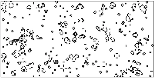
3. behavior is more complicated and appears random, but some repeated patterns are usually present (often in the form of triangles)(chaotic pattern).
4. in some respects these are the most complicated class; these behave in a manner somewhere in between Class II and III, exhibiting sec-tions both of predictable patterns and of randomness in their pattern formation(complex structures).
He observed that the behavior of a meaningful class of Cellular Automata by performing computer simulations of the evolution of the automata starting from random configurations. Wolfram suggested that the different behavior
13They prove that decide the class(from the wolfram’s four one) of membership of a
generic CA is an undecidable problem. Is not possible to design an algorithm that solve this problem.
of automata in his classes seems to be related to the presence of different types of attractors.
In figures 2.5 and 2.6 some elementary automata divided in their classes.14 Figure 2.5: Class 1 (a,b) and 2 (c,d) elementary cellular automata
(a) Rule 250 (b) Rule 254 (c) Rule 4 (d) Rule 108
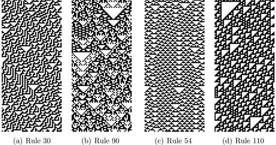
We can well see from these examples that automata from class 1 have all cells ending up very quickly with the same value, in a homogeneous state and automata from class 2 with a simple final periodic patterns. Class 3 appear to be chaotic and non-periodic and automata from class 4 have a mixed behaviour, complex-chaotic structures are locally propagated.
2.1.4.3 At the edge of Chaos
Class 4 automata are at the edge of chaos and give a good metaphor for the idea that the interesting complexity (like the one exhibit by biological entities and their interactions or analogous to the phase transition between solid and fluid state of the matter, is in equilibrium between stability and chaos [41].
Perhaps the most exciting implication (of CA representation of biological phenomena) is the possibility that life had its origin in the vicinity of a phase transition and that evolution reflects the process by which life has gained local control over a successively greater number of environmental parameters affecting its ability
to maintain itself at a critical balance point between order and chaos.
(Chris Langton - Computation at the edge of chaos. Phase transition and emergent computation - pag.13).
Figure 2.6: Class 3 (a,b) and 4 (c,d) elementary cellular automata
(a) Rule 30 (b) Rule 90 (c) Rule 54 (d) Rule 110
Langton in his famous paper, Computation at the edge of chaos: phase transition and emergent computation [41], was able to identify, by simply parametrizing the rule space, the various AC classes, the relation between them and to “couple” them with the classical complexity classes. He intro-duced the parameter λ [40] that, informally, is simply the fraction of the entries in the transition rule table that are mapped the not-quiescent state.
λ = K
N − n q KN where:
• K is the number of the cell states • N the arity of the neighborhood
• nq the number of rules mapped to the quiescent state qq
Langton’s major finding was that a simple measure is correlated with the system behavior: as it goes from 0 to 1 − K1(respectively the most homoge-neous and the most heterogehomoge-neous rules table scenario), the average behavior
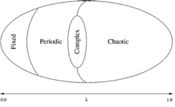
Figure 2.7: Relation between lambda parameter and the CA behaviors-Wolfram’s classes.
of the system goes from freezing to periodic patterns to chaos and functions with an average value of λ (see [41] for a more general discussion) are being on on the edge(see figure 2.7).
He studied a entire family of totalistic CA with k = 4 and N = 5 with λ varying in [0, 0.75]. He was able to determine that values of λ ≈ 0.45 raise up to class 4 cellular automata. A computational system must provide fundamental properties if it is to support computation. Only CA on the edge show these properties on manipulating and store information data. Here are the properties that a computational system as to provide:
Storage
Storage is the ability of the system of preserving information for arbi-trarily long times
Transmission
Transmission is the propagation of the information in the form of signals over arbitrarily long distance
Modification
Stored and transmitted information is the mutual possible modification of two signals.
Storage is coupled with less entropy of the system, but transmission and modification are not. Few entropy is associated with CA of Class 1 and 2 and high entropy with class 3. Class 4 is something in between, the cells cooperate and are correlate each other, but not too much otherwise they would be overly dependent with one mimicking the other supporting computation in all its aspects and requirements. Moreover class 4 CA are very dependent from the initial configuration opening to the possibility to encode programs in it.
2.1.4.4 Game of life
CA are suitable for representing many physical, biological, social and other human phenomena. But they are a good tool to study under which condi-tion a physical system supports the basic operacondi-tion constituting the capacity to support computation. The Game of life is a famous 2D cellular automa-ton of ’70s early studied (and perhaps proved) for its universal computation capacity.
Game of life - brief definition
The Game of Life (see figure 2.8) (GOL) [13] is a totalistic CA15 defined by :
• a 2-D lattice of square cells in an orthogonal grid, ideally infinite • Q = {0, 1} 2 states, and we can picture 1 as meaning alive and 0
dead (those interpretation come from the behaviour of the next-state function).
• X is the Moore neighborhood template.
• σ is the transition function and can be summarized :
– Birth: If the cell is in the state dead and the number of alive neighbors is 3 , then the cell state becomes alive (1).
– Survival : If the cell is in the state alive and the number of alive neighbors is 2 or 3 , then the cell state is still alive (1).
– Dead : If the cell is in the state alive and the number of alive neighbors is less than 2 or higher than 3 , then the cell state becomes dead (0).
GOL is a class 4 Wolfram’s taxonomy, rich complex structures, stable blocks and moving patterns come into existence even starting from a com-pletely random configuration.
15A totalistic cellular automaton is a cellular automata in which the rules depend only
Figure 2.8: GOL execution example.
A famous example block is the glider (see picture 2.9) that is a 5-step-period pattern that is capable of moving into the cellular space.
Game of life as a Turing machine
Every CA can be considered a device capable of supporting computation and the initial configuration can encode an input string (a program for ex-ample). At some point the current configuration can be interpreted as the result of the computation and decoded in a output string. But as we stated before in subsection 2.1.2.1 not all the computational device have the same computational power. So which is the one of the game of life? Life was proved can compute everything a universal Turing machine can, and under Turing-Church’s thesis, everything can be computed by a computer [9].
Figure 2.9: Glider in Conway’s game of life.
This raises a computational issue; given the Halting Theorem16the evolu-tion of Life is unpredictable (as all the universal computaevolu-tional systems) so
16There can not be any algorithm to decide whether, given an input, a Turing machine
it means that is not possible to use any algorithmically shortcut to anticipate the resulting configuration given an initial input. The most efficient way is to let the system run.
Life, like all computationally universal systems, defines the most efficient simulation of its own behavior [33]
2.1.5
Extension of the Cellular automata model
It is possible to relax some of the assumptions in the general characterization of CA provided in the ordinary CA definitions and get interesting results. Asynchronous updating of the cell, non homogenous lattice with different neighborhood or transition functions.
2.1.5.1 Probabilistic CA
Probabilist CA is are an extension of the common CA paradigm. They share all the basic concept of an ordinary homogeneous CA with an important difference in the transition function. σ is a stochastic-function that choose the next-state according to some probability distributions. They are used in a wide class of problems like in modelling ferromagnetism, statistical mechanics [26] or the cellular Potts model17
Cellular Automata as Markov process
Another approach in studying CA, even if it is probably not a practical way to study the CA is to see CA as a Markov process18. A Markov process, is a stochastic process that exhibits memorylessness 19and it means that the future state is conditionally independent20 of the past. This property of the process means that future probabilities of an event may be determined from the probabilities of events at the current time. More formally if a process has this property following equation holds:
P (X(tn) = x |X (t1) = x1, X(t2) = x2, . . . , X(tn−1) = xn−1) = P (X(tn) = x|X(tn−1 = xn−1)
17Is a computational lattice-based model to simulate the collective behavior of cellular
structures.
18Name for the Russian mathematician Andrey Markov best known for his work on
stochastic processes.
19Also called Markov property.
20Two event A and B are independent if P (AB) = P (A)P (B) or in other words that
In PCA analysis we are more interested in Markov chain because each cell has a discrete set of possible value for the status variable. In terms of chain a CA is a process that starts in one of these states and moves successively from one state to another. If the chain is currently in state si, than it evolve to state sj at the next step with probability pij.The changes of state of the system are called transitions, and the probabilities associated with various state changes are called transition probabilities usually represented in the Markov chain transition matrix :
M = p11 p12 p13 · · · p21 p12 p23 · · · p31 p32 p33 · · · .. . ... ... . ..
This could seems to be a good way to analyze a probabilistic CA but, a 10×10 small grid (common models model use grid 100×100 or larger) identify 210×10 possible states and the resulting matrix dimension is 210×10× 210×10, an indeed very large number.
2.2
GPGPU Technologies
GPGPU, acronym for General-purpose computing on graphics processing units, is a recent phenomenon wich consist in the utilization of a graph-ics processing unit (GPU21), which typically handles computation only for computer graphics and was optimized for a small set of graphic operation, to perform computation in applications traditionally handled by the cen-tral processing unit (CPU). Those operations (generation of 3D images) are intrinsically parallel, so, is not surprising if the underlying hardware has evolved into a highly parallel, multithreaded, and many-core processor. The GPU excels at fine grained, data-parallel workloads consisting of thousands of independent threads executing vertex, geometry, and pixel-shader program threads concurrently. Nowadays, the GPUs are not limited to its use as a graphics engine; there is a rapidly growing interest in using these units as parallel computing architecture due to the tremendous performance available in them. Currently, GPUs outperform CPUs on floating point performance and memory bandwidth, both by a factor of roughly 100 [48], easily reaching computational powers in the order of teraFLOPS. GPU works alongside the CPU providing an heterogeneous computation, simply offloading compute-data-intensive portion of program on GPU using it as co-processor highly specialized in parallel tasks. Plus since 2006, date when Nvidia has intro-duced CUDA, is extremely simple to program these kind of devices for general purpose tasks, although before that date this goal was achieved dealing di-rectly with the graphic API using shaders with all the related constraints such as lack of integers or bit operations.
2.2.1
Why GPU computing?
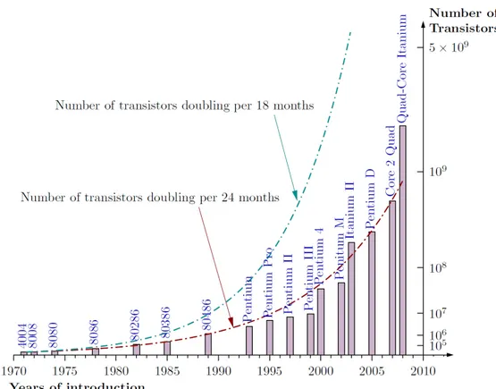
Traditionally performance improvements in computer architecture have come from cramming ever more functional units onto silicon, increasing clock speeds and transistors number. Moores law [28] states that the number of transistors that can be placed inexpensively on an integrated circuit will double approximately every two years.
21Graphic processing unit, term conied by Nvidia in the mid-nineties, and now the most
Figure 2.10: Moore’s Law and intel family CPU transistors number history. Coupled with increasing clock speeds CPU performance has until recently scaled likewise. But this trend cannot be sustained indefinitely or forever. Increased clock speed and transistor number require more power and generate more heat. Although the trend for transistor densities has continued to steadily increase, clock speeds began slowing circa 2003 at 3 GHz. If we apply Moore’s law type thinking to clock-speed performance, we should be able to buy at least 10 GHz CPUs. However, the fastest CPU available today is 3.80 GHz At same point the performance increase fails to increase proportionally with the added effort in terms of transistors or clock speed because efficient heat dissipation and increasing transistor resolution on a wafer becomes more important and challenging (there will be still the physical limit of dimension for each transistor, the atom). The heat emitted from the modern processor, measured in power density (cmW2) rivals the heat of a nuclear reactor core [27].
Figure 2.11: Temperature CPUs
But the power demand did not stop in these year, here the necessity of switching on parallel architectures, so today the dominating trend in com-modity CPU architectures is multiple processing cores mounted on a single die operating at reduced clock speeds and sharing some resources. Today is normal to use the so-called multi-core (2,4,8,12) CPUs on a desktop PC at home.
2.2.2
From Graphics to General Purpose Computing
The concept of many processor working together in concert in not new in the graphic field of the computer science. Since the demand generated by entertainment started to growth multi-core hardware emerged in order to take advantage of the high parallel task of generating 3D image. In computer graphics, the process of generating a 3D images consist of refreshing pixels at rate of sixty or more Hz. Each pixel to be processed goes through a number of stages, and this process is commonly referred to as the graphic processing pipeline. The peculiarity of this task is that the computation each pixel is independent of the other’s so this work is perfectly suitable for distribution over parallel processing elements. To support extremely fast processing of large graphics data sets (vertices and fragments), modern GPUs employ a stream processing model with parallelism. The game industry boosted the development of the GPU, that offer now greater performance than CPUs and are improving faster too (see Figure 2.13 and 2.12). The reason behind the discrepancy in floating-point capability between CPU and GPU is that GPU is designed such that more transistors are devoted to data processing rather than caching and flow control.
The today’s Top 500 Supercomputers22 ranking is dominated by mas-sively parallel computer, built on top of superfast networks and millions of sequential CPUs working in concert but as the industry is developing even more powerful, programmable and capable GPUs in term of GFlops we see that they begin to offer advantages over traditional cluster of computers in terms of economicity and scalability.
Figure 2.12: Intel CPUs and Nvidia GPUs memory bandwidth chart
2.2.2.1 Traditional Graphics Pipeline
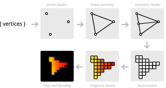
A graphics task such as rendering a 3D scene on the GPU involves a sequence of processing stages (i.e. shaders) that run in parallel and in a prefixed order, known as the graphics hardware pipeline23 (see Figure 2.14).
The first stage of the pipeline is the vertex processing. The input to this stage is a 3D polygonal mesh. The 3D world coordinates of each vertex of
22
http://www.top500.org/statistics/list/
23
Figure 2.13: Intel CPUs and Nvidia GPUs (single and double precision) Peak G/FLOPS chart
the mesh are transformed to a 2D screen position. Color and texture coor-dinates associated with each vertex are also evaluated. In the second stage, the transformed vertices are grouped into rendering primitives, such as tri-angles. Each primitive is scan-converted, generating a set of fragments in screen space. Each fragment stores the state information needed to update a pixel. In the third stage, called the fragment processing, the texture co-ordinates of each fragment are used to fetch colors of the appropriate texels (texture pixels) from one or more textures. Mathematical operations may also be performed to determine the ultimate color for the fragment. Finally, various tests (e.g., depth and alpha) are conducted to determine whether the fragment should be used to update a pixel in the frame buffer. Each shader in the pipeline performs a basic but specialised operation on the vertices as it passes. In a shader based architecture the individual shader processors exhibit very limited capabilities beyond their specific purpose. Before the advent of CUDA in 2006 most of the techniques for non-graphics computa-tion on the GPU took advantages of the programmable fragment processing stage. The steps involved in mapping a computation on the GPU are as follows:
Figure 2.14: Typical graphic pipeline
1. The data are laid out as texel colors in textures;
2. Each computation step is implemented with a user-defined fragment program. The results are encoded as pixel colors and rendered into a pixel-buffer24;
3. Results that are to be used in subsequent calculations are copied to textures for temporary storage.
The year 2006 marked a significant turning point in GPU architecture. The G80 was the first NVidia GPU to have a unified architecture whereby the different shader processors were combined into unified stream processors. The resulting stream processors had to be more complex so as to provide all of the functionality of the shader processors they replaced. Although research had been carried out into general purpose programming for GPUs previously, this architectural change opened the door to a far wider range of applications and practitioners. More in detail GPU are well-suited for problems highly data-parallel in wich the same code is executed on many data elements at the same time (SIMD paradigm25 or more generally as a CRCW PRAM machine26).
24A buffer in GPU memory which is similar to a frame-buffer.
25Single Instruction, Multiple Data: elements of short vectors are processed in parallel.
To be clear CUDA paradigm is SIMT: Single Instruction, Multiple Threads
2.2.3
CUDA
CUDA (Compute Unified Device Architecture) is a parallel computing plat-form and programming model created by NVIDIA and implemented by the graphics processing units (GPUs) that they produce. A platform that al-low the developers to use an high-level programming language to exploit the parallel power of the hardware in order to solve complex computational prob-lems in a more efficient way than on a CPU. CUDA is attractive because is a complete system(software and hardware model map well onto each other aiding the developer comprehension), from silicon to high-level libraries and a growing experience exists providing a valuable resource to developers.
Figure 2.15: Cuda Software Stack
CUDA expose three level of components to an application (See figure 2.15):
1. Cuda Driver :
• Distinct from graphics driver. The only purpose of this component is to provide the access to the GPU’s general purpose functional-ities.
2. CUDA Runtime:
• Built on top of the CUDA Driver, provide an higher level of ab-straction making the code less cumbersome especially as far as the complexity of host code for kernel launches is concerned.
3. CUDA Libraries:
• Built on top of the CUDA Runtime, Is a collection of Libraries (CUBLAS, CUSP, CUFFT, Thrust etc.)27 providing full-suitable state of the art implementation of algorithms for a wide range of applications.
2.2.3.1 CUDA Programming model
CUDA programming model is designed to fully expose parallel capabilities of NVIDIA GPUs. Even though the language is devoted to general purpose computing, it still requires the programmer to follow a set of paradigms aris-ing from the GPU architecture. CUDA provides a few easily understood abstractions that allow the programmer to focus on algorithmic efficiency and develop scalable parallel applications by expressing the parallelism ex-plicitly. It provides three key abstractions as hierarchy of thread groups, shared memories, and synchronization barrier that provide a clear parallel structure to conventional C code for one thread of the hierarchy.
Figure 2.16: Automatic Scalability
The abstractions guide the programmer to partition the problem into coarse sub-problems that can be solved independently in parallel, and then
27For example CUFFT provides an interface for computing Fast Fourier Transform up to
Figure 2.17: Grid of thread blocks
into finer pieces that can be solved cooperatively in parallel. The program-ming model scales transparently to large numbers of processor cores: a com-piled CUDA program executes on any number of processors, and only the runtime system needs to know the physical processor count (See figure 2.16).
2.2.3.2 CUDA Threads and Kernels
A GPU can be seen as a computing device that is capable of executing an elevated number of independent threads in parallel. In addition, it can be thought of as an additional coprocessor of the main CPU (called in the CUDA context Host). In a typical GPU application, data parallel-like portions of the main application are carried out on the device by calling a function (called kernel) that is executed by many threads. Host and device have their own separate DRAM memories, and data is usually copied from one DRAM to the other by means of optimized API calls.
CUDA threads can cooperate together by sharing a common fast shared-memory, implemented using fast DRAM memory similar to first level cache, eventually synchronizing in some points of the kernel, within a so-called thread-block, where each thread is identified by its thread ID as illustrated by Figure 2.17. In order to better exploit the GPU, a thread block usually contains from 64 up to 1024 threads, defined as a three-dimensional array
of type dim3 (containing three integers defining each dimension). A thread can be referred to within a block by means of the built-in global variable threadIdx. While the number of threads within a block is limited, it is pos-sible to launch kernels with a larger total number of threads by batching together blocks of threads by means of a grid of blocks, usually defined as a two-dimensional array, which is also of type dim3 (with the third component set to 1). In this case, however, thread cooperation is reduced since threads that belong to different blocks do not share the same memory and thus can-not synchronize and communicate with each other. As for threads, a built-in global variable, blockIdx, can be used for accessing the block index within the grid. Threads in a block are synchronized by calling the syncthreads() function: once all threads have reached this point, execution is resumed nor-mally. As previously reported, one of the fundamental concepts in CUDA is the kernel. This is nothing but a C function, which once invoked is per-formed in parallel by all threads that the programmer has defined. To define a kernel, the programmer uses the global qualifier before the definition of the function. This function can be executed only by the device and can be only called by the host. To define the dimension of the grid and blocks on which the kernel will be launched on, the user must specify an expression of the form <<< Grid Size, Block Size >>>, placed between the kernel name and the argument list, such as in the following simple example:
1 // Kernel definition
2 __global__ void VecAdd(float* A, float* B, float* C)
3 {
4 int i = threadIdx.x;
5 C[i] = A[i] + B[i];
6 }
7 int main()
8 {
9 ...
10 // Kernel invocation with N threads 11 VecAdd<<<1, N>>>(A, B, C);
12 }
The above code first defines a kernel called VectAdd which will run on all N threads, with the aim to compute in the i-th position of the vector C, the sum of vectors A and B. Assuming that all three vectors have dimension N, each thread in parallel will be the sum of a position. For example, the thread with ID = 2 will calculate the sum of A[2] + B[2] and store the result in C[2].
2.2.3.3 Memory hierarchy
In CUDA, threads can access different memory locations during execution. Each thread has its own private memory, each block has a (limited) shared memory that is visible to all threads in the same block and finally all threads have access to global memory. In addition to these memory types, two other read-only, fast on-chip memory types can be defined: texture memory and constant memory. In CUDA, memory usage is crucial for the performance. For example, the shared memory is much faster than the global memory and the use of one rather than the other can dramatically increase or de-crease performance. By adopting variable type qualifiers, the programmer can define variables that reside in the global memory space of the device (with device ) or variables that reside in the shared memory space (with shared ) that are accessible only from threads within a block. Typical latency for accessing global memory variables is 200-300 clock cycles, com-pared with only 2-3 clock cycles for shared memory locations. In addition, global memory suffers from coalesced access problems, meaning that access to data should be performed in a particular fashion in order to fetch (or store) the data in the fewest number of transactions [49]. For these reasons, global memory access should be replaced by shared memory access when-ever possible. A CUDA C program can allocate global memory of the device in two different ways: through the linear memory or by means of CUDA arrays. CUDA arrays are types of memory optimized for texture manage-ment and were not exploited in this work. The more common adopted linear memory type is allocated using the cudaMalloc() function for allocating and cudaFree() function for memory de-allocation. Once allocated, it is possi-ble to transfer data from the Host memory to the global device memory, and vice-versa, by means of a special call to the cudaMemcpy() function. Specifically, cudaMemcpy() takes as parameters four kinds of memory type transfers: Host to Host, Host to Device, Device to Host and Device to De-vice. Note that all of the previous functions can only be called on the host. Figure 2.18 illustrates the GPU typical memory architecture. As shown, the fast on-chip shared memory is shared by all threads of a block.
As expected, to improve performance, variable access should be carried out in the shared memory rather than global memory, wherever possible. Un-fortunately, as Figure 2.18 shows, each variable or data structure allocated in shared memory must first be initialized in the global memory, and afterwards transferred in the shared one. This means that to copy data in the shared memory, global memory access must be first performed. So, the more this type of data is accessed, the more convenient is to use this type of memory, while for few accesses it is evident that shared memory might be somewhat
Figure 2.18: Typical memory architecture of a Graphic Processing Unit
degrading. As a consequence, a preliminary analysis of data access of the considered algorithm should be performed in order to evaluate the tradeoff and thus, convenience of using shared memory and how. As reported later in this work, the implementation with a hybrid allocation of variables results in an optimal performance, despite a total shared-memory version as it may be expected.
2.2.3.4 Programming with CUDA C
CUDA C is an extension of C language that permits to write programs for NVIDIA GPUs. With additional constructs and API functions, the program-mer is able to allocate and de-allocate memory on the video card (the device), transfer the data from the host device (host ), launch kernels, etc. The CUDA C extension is built on the basis of the CUDA API driver, a low-level library that allows one to perform all the above steps, but which of course is much less user-friendly. On the other hand, the CUDA API driver offers a higher degree of control and is independent of the particular language (e.g., C, For-tran, Java), being written in assembly language. A typical CUDA program can exploit the computing power of both the host (CPU and RAM) and the device (the GPU and memory devices). What follows is a classic pattern of a CUDA application:
1. Allocation and initialization of data structures in RAM memory; 2. Allocation of data structures in the device and transfer of data from
RAM to the memory of the device; 3. Definition of the block and thread grids; 4. Performing one or more kernel;
5. Transfer of data from the device memory to Host memory.
In addition, a CUDA application has parts that are normally performed in a serial fashion, and other parts that are performed in parallel.
2.2.4
OpenCL
Released on December 2008 by the Kronos Group28 OpenCL is an open standard for programming heterogeneous computers built from CPUs, GPUs and other processors that includes a framework to define the platform in terms of a host, one or more compute devices, and a C-based programming language for writing programs for the compute devices (see figure 2.19). One of the first advantages of OpenCL is that it is not restricted to the use of GPUs but it take each resource in the system as computational peer unit, easing the programmer by interfacing with them. Another big advantage is that it is open and free standard and it permit cross-vendor portability29. 2.2.4.1 Model Architecture
The architecture programming model’s follows the CUDA’s one but with different names.
28A standards consortium.
Figure 2.19: OpenCL heterogeneous computing. Work-items:
are equivalent to the CUDA threads and are the smallest execution entity of the hierarchy. Every time a Kernel is launched, lots of work-items (a number specified by the programmer) are launched, each one executing the same code. Each work-item has an ID, which is acces-sible from the kernel, and which is used to distinguish the data to be processed by each work-item.
Work-group:
equivalents to CUDA blocks, and their purpose is to permit commu-nication between groups of work-items and reflect how the work is or-ganized (usually oror-ganized as N-dimensional grid of work-groups with N ∈ {1, 2, 3}). As work-items, they are provided by a unique ID within a kernel. Also the memory model is similar to the CUDA’s one. The host has to orchestrate the memory copy to/from the device and ex-plicit;y call the kernel.
A big difference is in how a kernel is queued to execution on the accelerator. Kernels are usually listed in separate files the OpenCL runtime take that source code to create kernel object that can be first decorated with the pa-rameters on which it is going to be executed and then effectively enqueued for execution onto device. Here a brief description of the typical flow of an OpenCL application.
1. Contexts creation: The first step in every OpenCL application is to create a context and associate to it a number of devices, an available
OpenCL platform (there might be present more than one implementa-tion), and then each operation (memory management, kernel compiling and running) is performed within this context. In the example 2.2 a context associated with the CPU device and the first finded platform is created.
2. Memory buffers creation: OpenCL buffer Object are created. Those buffer are used to hold data to be computed onto devices.
3. Load and build program: we need to load and build the compute pro-gram (the propro-gram we intend to run on devices). The purpose of this phase is to create an object cl::Program that is associable with a context and then proceed building for a particular subset of context’s devices. We first query the runtime for the available devices and then load directly source code as string in a cl::Program:Source OpenCL object (see listing1 2.4).
4. In order a kernel to be executed a kernel object must be created. For a given Program there would exists more than one entry point (identi-fied by the keyword kernel 30). We choose one of them for execution specifying in the kernel object constructor
5. We effectively execute the kernel putting it into a cl::CommandQueue. Given a cl::CommandQueue queue, kernels can be queued using queue.-enqueuNDRangeKernel that queues a kernel on the associated device. Launching a kernel need some parameters (similar to launch configu-ration in CUDA, see section 2.2.3.2) to specify the work distribution among work-groups and their dimensionality and size of each dimension (see listing 2.1). We can test the status of the execution by querying the associated event.
Listing 2.1: OpenCL Queue command, kernel execution
1 cl_int err;
2 cl::vector< cl::Platform > platformList; 3 cl::Platform::get(&platformList);
4 checkErr(platformList.size()!=0 ? \\ 5 CL_SUCCESS:-1,"cl::Platform::get"); 6 cl_context_properties cprops[3] = 7 {CL_CONTEXT_PLATFORM, (cl_context_properties)( platformList[0])(), 0}; 8 cl::Context context(CL_DEVICE_TYPE_CPU,cprops,NULL, NULL,&err); 9 checkErr(err, "Conext::Context()");
Listing 2.2: OpenCL context creation
1 cl::Buffer outCL(context,CL_MEM_WRITE_ONLY |
2 CL_MEM_USE_HOST_PTR,hw.
length()+1,outH,&err);
3 checkErr(err, "Buffer::Buffer()");
Listing 2.3: OpenCL program load and build
1 std::ifstream file("pathToSourceCode.cl"); 2 checkErr(file.is_open() ? CL_SUCCESS:-1, "
pathToSourceCode.cl");std::string
3 prog( std::istreambuf_iterator<char>(file), 4 (std::istreambuf_iterator<char>()));
5 cl::Program::Sources source(1,std::make_pair(prog.
c_str(), prog.length()+1));
6 cl::Program program(context, source);
7 err = program.build(devices,""); 8 checkErr(err, "Program::build()");
Listing 2.4: OpenCL program load and build
1 cl::CommandQueue queue(context, devices[0], 0, &err); 2 checkErr(err, "CommandQueue::CommandQueue()");cl::
Event event;
3 err = queue.enqueueNDRangeKernel(kernel,cl::NullRange,
4 cl::NDRange(hw.length()+1), cl::NDRange(1, 1),NULL,&
event);
2.2.5
OpenACC
OpenACC is a new31 open parallel programming standard designed to en-able to easily to utilize massively parallel coprocessors. It consist of a series of pragma32 pre-compiler annotation that identifies the succeeding block of code or structured loop as a good candidate for parallelization exactly like OpenMP 33 developed by a consortium of companies34. The biggest advan-tage offered by openACC is that the programmer doesn’t need to learn a new language as CUDA or OpenCL require and doesn’t require a complete transformation of existing code. Pragmas and high-level APIs are designed to provide software functionality. They hide many details of the underlying implementation to free a programmer’s attention for other tasks. The com-piler is free to ignore any pragma for any reason including: it doesn’t support the pragma, syntax errors, code complexity etc. and at the same time it has to provide profiling tool and information about the parallelization(even if it is possible). OpenACC is available both for C/C++ and Fortran. In this docu-ment we will concentrate only on C/C++ version. An OpenACC pragma can be identified from the string ”#pragma acc” just like an OpenMP pragma can be identified from ”#pragma omp”. The base concept behind openACC is the offloading on the accelerator device. Like CUDA or openCL the ex-ecution model is host-directed where the bulk of the application execute on CPU and just the compute intensive region are effectively offloaded on ac-celerator35. The parallel regions or kernel regions, which typically contains work sharing work such as loops are executed as kernel (concept described in section 2.2.3.2 at page 29). The typical flow of an openACC application is orchestrated by the host that in sequence has to:
• Allocate memory on device. • Initiate transfer.
• Passing arguments and start kernel execution(a sequence of kernels can be queued).
• Waiting for completion.
31Release 1.0 in November 2011.
32A pragma is a form of code annotation that informs the compiler of something about
the code.
33The is a well-known and widely supported standard, born in 1997, that defines pragmas
programmers have used since 1997 to parallelize applications on shared memory multicore processor
34PGI, Cray, and NVIDIA with support from CAPS
35We don’t talk of GPU because here, accelerator is referred to the category of
• Transfer the result back to the host. • Deallocate memory.
For each of the action above there is one or more directive that actually implements the directives and a complete set of option permit to tune the parallelization across different kind of accelerators. For instance the parallel directive starts a parallel execution of the code above it on the accelerator, constricting gangs of workers (once started the execution the number of gangs and workers inside the gangs remain constant for the duration of the parallel execution.) The analogy between the CUDA blocks and between workers and cuda threads is clear and permit to easily understand how the work is effectively executed and organized. It has a number of options that permits to for example copy an array on gpu to work on and to copy back the result on the host side.
The syntax of a OpenACC directive is :
• C/C++ : #pragma acc directive-name [clause [[,] clause]...] new-line. • Fortran : !$acc directive-name [clause [[,] clause]...]
Each clause can be coupled with a number of clauses that modify the behavior of the directive. For example:
• copy( list )Allocates the data in list on the accelerator and copies the data from the host to the accelerator when entering the region, and copies the data from the accelerator to the host when exiting the region. • copyin( list ) Allocates the data in list on the accelerator and copies
the data from the host to the accelerator when entering the region. • copyout( list ) Allocates the data in list on the accelerator and copies
the data from the accelerator to the host when exiting the region. • create( list ) Allocates the data in list on the accelerator, but doesn’t
copy data between the host and device.
• present( list ) The data in list must be already present on the acceler-ator, from some containing data region; that accelerator copy is found and used.
2.2.5.1 Wait Directive
The wait directive causes the host program to wait for completion of asyn-chronous accelerator activities. With no expression, it will wait for all out-standing asynchronous activities.
• C/C++ : #pragma acc wait [( expression )] new-line • Fortran : !$acc wait [(expression)]
2.2.5.2 Kernel Directive
This construct defines a region of the program that is to be compiled into a sequence of kernels for execution on the accelerator device.
C/C++:
#pragma kernels [clause [[,] clause]...] new-line { structured block } Fortran:
!$acc kernels [clause [[,] clause]...] structured block
!$acc end kernels
2.2.5.3 Data Construct
An accelerator data construct defines a region of the program within which data is accessible by the accelerator. It’s very useful in order to avoid multiple transfers from host to accelerator or viceversa. If the same pointers are used by multiple directives, a good practice is to declare and allocate those pointers in a data construct and use them in parallel or kernel construct with the clause present [57].
Description of the clause are taken from the official documentation36.
2.3
WEB 2.0
In 2001 one of the most important companies of the time in the Internet world went bankrupt, the Webvan company. Webvan was intended to sell anything to anyone and everywhere; even though it was a company that was born from a business model quite inconsistent, it managed to collect 400 million dollars from venture capitals and following its founder was able to
36For a complete list of directive, constructs and pragmas consult the official