Efficient Scheduling for Heterogeneous Fractional Lambda Switching Networks

UNIVERSITY

OF TRENTO

DEPARTMENT OF INFORMATION AND COMMUNICATION TECHNOLOGY 38050 Povo – Trento (Italy), Via Sommarive 14

http://www.dit.unitn.it

Efficient Scheduling for Heterogeneous Fractional Lambda

Switching (F

λS) Networks

Thu-Huong Truong, Mario Baldi, Yoram Ofek

March 2007

Abstract— Efficient scheduling for heterogeneous fractional lambda switching (FλS) networks is required but challenging. A heterogeneous network implies bandwidth mismatch between links of varied bit rates. Moreover, when non-immediate forwarding (NIF) is used in FλS, it increases the scheduling complexity exponentially, while decreasing the blocking probability. Thus, NIF scheduling presents a serious challenge for an algorithm to be used in a large heterogeneous FλS

network. In this paper, an efficient scheduling algorithm that is combined with a flexible forwarding scheme is presented. The algorithm provides a full scheduling solution for an end-to-end request in heterogeneous FλS

networks. Furthermore, the algorithm has linear complexity in single-channel networks and quadratic complexity in multiple-channel WDM networks.

Index Terms— scheduling, search algorithms, fractional

lambda switching, pipeline forwarding, optical networks

I. INTRODUCTION

The Internet is experiencing fast exponential growth and diversity of bandwidth usages primarily from multimedia and converged services. Such applications require end-to-end quality of service (QoS). One of the promising end-to-end QoS solution is through the deployment of fractional (or sub-) lambda switching (FλS) [1]-[5]. FλS is a scalable switching solution based on the use of UTC (coordinated universal time) with pipeline forwarding, which is the main context of this paper. Under the pipeline forwarding principle packets are forwarded in time frames (TFs) in a “lock-step” manner across the route. TFs are “virtual containers” to be transported at a predefined scheduled request. FλS enables deterministic performance guarantees, low cost, switching scalability, and flexible bandwidth provisioning.

Pipeline forwarding can be performed in two manners at a FλS switch: (1) immediate forwarding - IF or (2) non-immediate forwarding – NIF (see Section II.B). We address the NIF scenarios since NIF provides higher scheduling flexibility compared to the simple IF, and consequently,

significantly reduces the blocking probability [2]. However, using NIF is a challenge for a scheduling algorithm since complexity is much higher.

Moreover, end-to-end connections can involve heterogeneous links along their routes, where bit rates, TF durations and forwarding buffers can be varied from link to link. This heterogeneity makes scheduling problem more complicated since bit-rate mismatch between high speed backbones and low speed access links can be substantial.

In this paper, we define a suitable forwarding scheme called Inter-TF forwarding for arranging flows at a switch where the bit rates of its input and output are mismatched. We then develop a scheduling algorithm for flows that require bandwidth of a single TF. The addressed scenarios are heterogeneous single-channel and multiple-channel (WDM) optical networks using NIF.

The proposed scheduling algorithm called HeSS (efficient

Heterogeneity-oriented Survivor-based Search) operates over

a trellis graph that is specially constructed to reflect the heterogeneity of FλS networks. HeSS reliably searches for the schedule with best QoS delay metrics. Motivated by the Viterbi algorithm [7], HeSS allows dynamic programming and helps searching the NIF schedule space with acceptable complexity, also on multiple lambdas (WDM). Compared to the well known Dijkstra algorithm [8][9], the HeSS algorithm can be naturally implemented both in a distributed and centralized manner, by exploiting the topological structure of the trellis (in the time-space domain). Whereas, Dijkstra is traditionally performed in the space domain, and is not easily performed on each switch of the FλS route in a distributed manner (see [11] for more details).

The paper is organized as follows: Section II presents heterogeneous FλS network principles, introduces the network model and shows the way leading to our proposed solution. In Section III and IV, scheduling for the case of single-TF request in a single-channel, heterogeneous network and an extension to WDM heterogeneous networks are shown, respectively. Finally, further works are discussed in Section V.

Efficient Scheduling for Heterogeneous

Fractional Lambda Switching (FλS) Networks

Thu-Huong Truong♦ , Mario Baldi∗, Yoram Ofek♦

♦_{Department of Information and Communication Technology}

University of Trento, Italy Email: (huong.truong, ofek)@dit.unitn.it

∗_{Control and Computer Engineering Department}

Politechnico di Torino, Italy Email: mario.baldi@polito.it

A. Timing principle

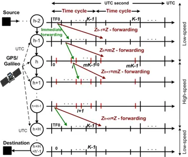
In this sub-section, we briefly introduce to the FλS network principles. A detail background of FλS can be found in [2]. FλS networks use common time reference (CTR) that is commonly realized by using UTC (coordinated universal time). UTC is available everywhere through GPS and Galileo in the near future with accuracy that is well below 1µs.

A standard UTC second is divided into equal time frames (TFs), which are grouped into time cycles (TCs), such that, multiple contiguous TCs are equal to one UTC second (Figure 1). TFs are used as containers to align and forward multi-protocol packets. The TF capacity is calculated according to its duration and the link bit rate. In this work there are K TFs per TC and all links are having the same TC duration; while the value K may be varied on links if the network is heterogeneous (i.e. links with different bit rates) or the value K may be constant if the network is homogeneous (i.e. links with the same bit rates).

B. Pipeline Forwarding

The fundamental principle of FλS network operation is pipeline forwarding (PF), in which packets are forwarded in TFs with a predefined forwarding schedule that is responsive to UTC and without header processing. Consequently, TFs can be viewed as virtual containers of packets. One TF then is treated as one uniform unit during the transportation. The necessary condition for pipeline forwarding is having delay among inputs of FλS switches as an integer number of TFs. In order to realize this all incoming TFs should be aligned with UTC. Without loss of generality, in this work we assume the availability of this alignment operation and ignore the propagation delay.

Pipeline forwarding delay is the delay of one hop measured in TFs between the inputs of two neighboring switches. In fact, the forwarding delay comprises of the propagation delay and the necessary UTC alignment delay (which we assume to be zero in the following analysis) and the Zj-forwarding

delay, which is the scheduling delay that is due to holding the

packets content of an input TF at switch j for the duration of Zj

output TFs before forwarding to the next FλS switch on the route.

In homogeneous network scenarios [1]-[5] and [11], homogeneous links conceptually enable us to idealize the shortest forwarding delay to 0, however in heterogeneous networks, we need to practically address the heterogeneity of TFs and link bit rates at the input and output of a switch discussed in this paper by providing a new definition of the pipeline forwarding:

Definition 1

For Zj-forwarding:

1. Zj =1 – Immediate Forwarding (IF): given that the TF at

the input and output of a switch are aligned, upon the end of an input TF to switch j, data of the TF is forwarded to the next switch during the next output TF.

forwarded to next switch with delay from 1 to Zj output

TFs on the output link. Where:

Kj: Number of TFs per TC at the output link of switch j

The case of Zj=Kj is called full forwarding (FF) since the

incoming TF can be forwarded in any TF in one TC span. It is obviously seen that exploiting IF provides much smaller freedom in selecting TF sequence at each switch. Meanwhile, the case of FF is trivial for scheduling since it can always pick out schedules as long as resource is still available. Therefore, this work focuses on NIF, since it brings more scheduling flexibility and scalability, reducing blocking probability, less buffer usage and increasing network utilization.

C. Network model

This work addresses a fractional lambda switching (FλS) network with an arbitrary topology, where each optical link transports one or more optical channels (lambdas) with defined transmission bit rates.

Figure 1- Time structure, pipeline forwarding in a heterogeneous network model

As illustrated in Figure 1, our network model focuses on a route carrying traffic of a flow from source to destination via multiple FλS switches. The route can bear multiple links with different bit rates. In FλS, routes are determined for any flow using existing routing protocols. FλS then focuses on the manner of (pipeline) forwarding the packets on that route. Hence, we will only study here the FλS network problem: (1) on one predefined route (without route selection) with a predefined number of FλS switches, (2) without propagation delay and alignment delay.

Without loss of generality, a flow is set-up over a route starting with a uniformly low bit rate domain of h switches (or

homogeneous domain) connecting with a high bit rate

domain of h’ switches again. Therefore, the model has one low-to-high-bit-rate interface, and one high-to-low-bit-rate interface. The analysis can be easily extended to a more general case of any number of low-to-bit-rate and high-to-low-bit-rate points separated by homogeneous domains.

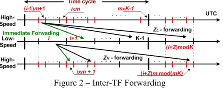
An effect of a heterogeneous network with different link speeds and FλS parameters (i.e: numbers of TFs per TC) is that a requested flow of deterministic bandwidth will experience varied resources along the route. It leads to a forwarding solution described in the following sections II.D. D. Pipeline forwarding scheme in heterogeneous networks To handle forwarding at FλS switches, connecting heterogeneous links with mismatched bit rates, the switches need to possess the functionality of multiplexing or demultiplexing packets from multiple lower bit-rate links to a higher bit-rate link or vice versa. From the perspective of pipeline forwarding, the bit-rate mismatch at those switches motivates us to come up with a new forwarding technique for forwarding packets from an input TF to an output TF:

inter-TF forwarding in order to cover the change in inter-TF attributes

along a route. Inter-TF Forwarding technique is described as follows:

Based on a general assumption of fixed time cycle (TC) duration, the time frame size on the output channel is the same as on the input channels, however, due to the higher capacity of the output channel, the time frame duration is proportionally shorter. Inter-TF Forwarding means: at switch j, data content of a shorter input TF is forwarded to any longer output TF in the range of Zj-forwarding and vice versa. Figure

2 illustrates how the forwarding procedure executes at high-to-low bit-rate and low-to-high bit-rate interfaces. Assume that there is a capacity difference of m times between high and low bit-rate links.

Figure 2 – Inter-TF Forwarding

The forwarding buffer range for the slow link is managed to be ZL, while the range for the fast link is ZH= m⋅ZL due to TFL

= mTFH. The policy comes from the idea that the forwarding

flexibility should be kept constant among links:

H H L L K Z K Z = ,

when TC=const. In details, upon the high-to-low interface, data of a shorter incoming TF after fully received from a high rate link can be forwarded to any longer TF of the low bit-rate link with delay from 1 to ZL of TFL.

Thus, at this interface, the forwarding changes to (ZL

=Z)-forwarding. Due to the difference between the time scales of the high and low bit-rate links, data of the incoming TF can be forwarded earliest (according to Definition 1) at the next TFL

after its arrival.

Upon the low-to-high interface, there is an implicit groom of m input links to an output link (due to the m-time bit-rate mismatch). Thus data of those m links at the output link is to be buffered and mapped to a combined wide range of (ZH=

m⋅ZL=m⋅Z) TFH to accommodate forwarding for each TFL of

those m links. The forwarding scheme changes to (ZH= m⋅Z)

-forwarding.

E. NIF and its exponential growth in scheduling possibilities

Definition 2

Available TF - a TF at an output of a switch that can

participate in carrying packets of a requested flow.

Choice - a choice is an available output TF selected for a

given flow for which a set-up request arrives at a switch. A choice is restricted by the Zj-forwarding constraint of the

switch

Schedule - a schedule is a sequence of choices over a

predefined route of multiple switches.

Blocking of a schedule - a schedule is blocked at switch j

when no choice is possible on that switch to advance the schedule to the next switch.

For NIF, sufficient bandwidth (available TFs) on every switch does not guarantee a non-blocking schedule to setup a flow, due to the mapping range restricted within Zj TFs forwarding.

TFs on a link in general are assumed to be randomly available since the flows are stochastically set up and released; thus all its available TFs may happen to be out of the Zj-range for the

considered request from the previous switch. Moreover, scheduling for NIF is a complicated task due to the large space of possible schedules:

∏

= − = ⋅ ⋅ 1 1 0 1 1 0 ... n j j n K Z Z Z K for

single-channel heterogeneous networks,

∏

= ⋅ ⋅ 1 1 0 n j j n Z K C for

WDM heterogeneous networks, where n=h+H+h’ is the number of switches over the route according to the network model (proofs derived from [11]). The space of possible schedules that is exponential in size of the network n is a nontrivial problem for any scheduling algorithm to cope with and is a factor to limit the network scale.

III. HESS -SCHEDULING ALGORITHM AND COMPLEXITY ANALYSIS

In this section, we first schedule flows that request bandwidth of single-TF in the scenario of single-channel heterogeneous networks. As mentioned in the network model above, scheduling is performed along a route carrying traffic of a flow from source to destination via multiple switches (i.e. h+H+h’ switches). The route is defined as follows:

- h-switch low bit-rate domain (j: 0Æh-1) preceding point (h/Gr): a Gbps, K TFs per TC, (Zj=Z)-forwarding

- H-switch high bit-rate domain (j: hÆ h+H-1) between the low-to-high (h/Gr) and high-to-low (h+H/DeGr) point: (m·a) Gbps and (m·K) TFs per TC, (Zj=m⋅Z)-forwarding

(Zj=Z)-forwarding

- (m·Z)-forwarding be used at point (h/Gr), and Z-forwarding be used at point (h+H /DeGr)

A. Construction of trellis graph for the network model The synchronous forwarding upon a fixed set of TFs at each node from Source to Destination brings an analogy to the trellis graph characteristics. Trellis vertices can represent the schedule choices. A trellis transition between a vertice pair of two sequential stages symbolizes Zj-forwarding while its

metric is used to select best QoS schedules in terms of delay.

Figure 3- Trellis example with Z =2, K=4, m=2 Based on the assumed route model above, we can describe the trellis diagram as (h+H+h’) columns corresponding to (h+H+h’) switches along a route, K rows for low-bit-rate domains corresponding to K TFs per TC, and (m⋅K) rows for high-bit-rate domain corresponding to (m⋅K) TFs per TC as illustrated in Figure 3. Each vertex of the trellis diagram is called a STATE

TF

• The H stages include m·K states, while the other stages include K states. A transitions between homogeneous links is allowed from a state i to a state in the range: [i+1,(i+Z)mod K] if in low-bit-rate domain and [i+1,(i+m⋅Z)mod(m⋅K)] if in high-bit-rate domain (F-i) • Transitions from a state i at the stage before the

low-to-high point (h/Gr) are possible to states at stage (h/Gr) in the range [(i⋅m)+1,(i⋅m+m⋅Z)mod (m⋅K)]. Therefore, each state of point (h/Gr) has Z transitions to itself from states at

low point (h+H/DeGr) are possible to states at stage (h+H /DeGr) in the range

(

   

(

)

)

Operating over the heterogeneous trellis diagram constructed in III.A, HeSS algorithm (efficient Heterogeneity-oriented

Survivor-based Search) computes to search potential

schedules stage by stage by using dynamic programming until the final stage is reached. HeSS can be formalized as follows:

Definition 3

Path: a trellis curve P from S to a state i on stage j (

TF

Branch metrics:

µ

(defined in section II.B) measured in TF of the first hop.

Accumulated path metric: total delay summed up on a path

by branch metrics from S to the considered state:

µ

( )

P

Survivor: the smallest accumulated-metric path among the

ones incident to the considered state

Path Filtration

The HeSS algorithm uses the technique of Path Filtration. At each stage j ∈ trellis graph, a minimized set of paths (a set of survivors) is selected by path filtration, with:

- Extending the survivor set from the previous stage by combining each with the current stage’s transitions

- Keeping at most one path, called survivor for each free state (available TF) and filtering out all other paths. - Filtration computes for each TF i with a comparison loop P is a set of survivor from previous stage, P[k]=NIL means state k has no survivor (no scheduling possible via k), P’ is a newly computed survivor set, 1≤ Db(k,i) ≤ Zj is the number of

output TFs delayed from P[k] to TF i. After all loops for each TF, a set of survivors is determined for stage j, and ready for path filtration at stage j+1.

PATH-FILTRATION (j,Kj,Zj)

1. For each state i ∈ stage j 2. For each survivor P[k] ∈ P

3. If, µ(P[k])+ µb ≤ µ(P’[i]), with µb Å Db(k,i)· j K K0 4. then µ(P’[i])= µ(P[k])+ µb P’[i] Å {P[k],i} 5. P Å P’ HeSS Algorithm 1. Do PATH-FILTRATION (j,Kj,Zj) j: 0Æ h-1, ∀ Kj=K, ∀ Zj=Z

2. At low-to-high interface (i.e stage h/Gr), with the forwarding range as (F-ii)

3. Do PATH-FILTRATION (j,Kj,Zj)

j: h+1Æ h+H-1, ∀ Kj= m⋅K, ∀ Zj= m⋅Z

4. At high-to-low interface (i.e stage h+H/DeGr), with the forwarding range as (F-iii)

Do PATH-FILTRATION (h+H/DeGr, K, Z).

5. Do PATH-FILTRATION (j,Kj,Zj)

j: h+HÆ h+H+h’-1, ∀ Kj=K, ∀ Zj=Z

6. Among the final survivor paths after 5, the one with smallest delay is chosen as the schedule.

Notice that only reachable available states called involved

states are involved in the searching procedure. It happens

from the fact that there can be busy TF or available TFs but unschedulable due to being out of NIF range, thus can not be reached by any scheduled state of the previous stage. This fact reduces the algorithm computational steps accordingly as network load increases.

C. HeSS Property

Thanks to Path Filtration attributes that filters undesired paths on the way of forward-dynamic-programming searching, the HeSS algorithm guarantees to always find at least one schedule whenever such a schedule exists. Moreover, HeSS returns the same scheduling outcome as what the exhaustive search algorithm can find out (the proof for this property can be taken directly from the proof in [11] in which homogeneous environment is investigated. Since the survivor selection mechanism for each state is similar between homogeneous and heterogeneous scenarios, the proof [11] still holds for this heterogeneous context). Possessing those properties above, HeSS avoids the impractically exponential complexity of the exhaustive search algorithm, as it has a linear complexity as shown in the following analysis.

D. Complexity analysis

In this subsection, the complexity of HeSS is analyzed over the assumed network model to show how efficiently it can perform in a certain scale of networks.

Since the HeSS computation is memoryless, in the sense that computation at a stage j is based solely on stage j-1, HeSS operation over the network model III.A can be seen as the sequential execution of five independent operations, each involving the application of HeSS to the five sub diagrams shown in Figure 3.

In a sub diagram having h switches (j: 0Æ h-1), (Zj

=Z)-forwarding, (Kj=K) TFs per TC, the worst case where all TFs

are available, complexity of HeSS is given (proof in [11]):

X(h,K,Z) = (h-1)⋅K⋅Z (1)

Consequently, the complexity of the scheduling computation for the assumed network model can be derived directly from the complexity (1) by applying (1) to the five sub diagrams, thus obtaining:

X = X(h,K,Z) + X(2,m⋅K,m⋅Z) + X(H-1, m⋅K, m⋅Z)

+ X(2,K,m⋅Z) + X(h’-1,K,Z) (2) The big O complexity finally is:O

(

(

)

)

The complexity shows the HeSS algorithm to be efficient to find out an optimal solution alike exhaustive approach, but with acceptable complexity linear in the size of networks (i.e.

h, K and Z). In the general implementation (linear search), the Dijkstra algorithm takes up to steps O(V2_{) for a graph}

{V,E}.Even for a sparse graph (e.g: not a full trellis, with small Zj, making the number of edges small) in which the

Dijkstra algorithm can utilize a priority queue with a binary heap, its complexity is O((V+E)logV) [9]. Both complexity figures are considerably greater than our solution’s O(E). (In our full trellis: the number of vertices is V= (h+m⋅H+h’)⋅K, and number of edges is E ~ (h+m⋅H+h’)⋅K⋅Z). Therefore, HeSS is capable of efficiently dealing with large-scale networks.

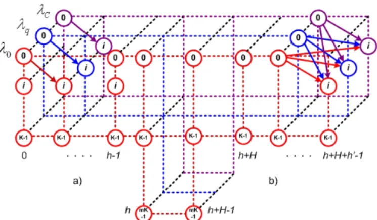
IV. EXTENDING HESS TO WDM HETEROGENEOUS NETWORKS

FλS is working towards ultra-scalable switching and efficient bandwidth provisioning via being well coupled with WDM. Real-time provisioning implies that wavelength should be assigned dynamically depending on the network state.

The following extends the HeSS scheduling algorithm to the scenario of multiple-channel (WDM) heterogeneous FλS networks. The scheduling in this scenario deals with the issue of wavelength and time frame assignment (WTA) with the major difference stemming from the nature of NIF (as specified using the parameter Z). The scheduling feasibility in this case is related to the availability of capacity on a wavelength during a given TF. Therefore, the objects dealt with by our scheduling algorithm here are bi-dimensional resources, given by pairs of

(

TF

,

λ

)

Figure 4 – Trellis diagram in a) no-wavelength-conversion, b) full wavelength conversion

Definition 4

State j

(

)

i

TF

λ

λ

(

)

i

TF

λ

λ

Choice - a choice is an available output TF on a wavelength

selected for a packet flow for which a set-up request arrives at a switch. A choice is restricted by the Zj-forwarding constraint

of the switch.

Schedule - a schedule is a sequence of choices of a specific

wavelength and a TF at each network switch, on a predefined route of multiple switches

Instead of the bi-dimensional trellis deployed in the previous case, a tri-dimensional one is required for the WDM case, features C planes

(

λ

,..,

λ

.,

λ

)

grown C times with respect to the single-wavelength case, i.e., N = C⋅K. The trellis diagram for this scenario is illustrated in Figure 4.

A. WDM with no wavelength conversion

We assume here that switches do not support any wavelength conversion capability. Hence wavelength continuity must be guaranteed end-to-end. The scheduling problem can be seen as the combination of a wavelength assignment (WA) and time frame assignment (TA) sub-problem. Several WA algorithms are proposed in literature such as first-fit, least-loaded [6] , most-used, least-used, min-product, max-sum etc. we suggest applying here the Least-Loaded selection algorithm where the load of a wavelength is measured as the minimum number of available TFs counted over each link on the route. The wavelength with the highest load metric will be selected. This assignment policy will balance the load (the used lambda fractions) on all wavelengths, thus potentially reduce the blocking probability [6]. With the disjoint

approach, the WA algorithm is run first to select a

wavelength, then follows TF searching on that lambda plane. With the joint approach, a wavelength is selected based on specific information from the HeSS algorithm, i.e., upon the delay of the best schedule among the ones found separately on each lambda.

Derived from (2), complexity analysis starts with a h-switch homogeneous domain is linear in the size of h, K, Z, C:

X(h,K,Z,C) = (h-1)⋅K⋅Z⋅C (3)

The complexity for the overall heterogeneous route is described in formula (5).

B. WDM with limited wavelength conversion

Assume that switches have limited wavelength conversion capabilities: each wavelength can be converted to one of R adjacent wavelengths, R ≤ C, in a contiguous wavelength selection fashion (R=C - full wavelength conversion). The

involved states (mentioned in III.B) in this 3-D trellis

diagram are defined not only if the state j

(

)

i

TF

λ

available TF reachable under NIF range but also if its wavelength convertible from the wavelength of the previous state under wavelength conversion constraint R.

HeSS is applied in the way that it searches all involved

states in the 3-D trellis diagram, progress at each state the

path with minimum accumulated delay (the sum of metrics µb). The metric µb can be constructed as a weighted sum of

three submetrics, i.e., delay, distance, and load. If the weight selected for one submetric, say delay, is much larger than the others, the schedule is selected mainly according to the delay and the others are used only to select among equal-delay paths.

Complexity of HeSS for a homogeneous domain is given as:

X(h,K,Z,R,C) = (h-1)⋅K⋅Z⋅C⋅R (4)

The complexity is linear in size of h,K and Z. If R~C, we have quadratic complexity in the size of C [10].

derived using (3) or (4), thus obtaining:

X = X(h,K,Z,R,C) + X(2,m⋅K, m⋅Z,R,C) + X(H-1,m⋅K,m⋅Z,R,C) + X(2,K, m⋅Z,R,C) + X(h’-1,K,Z,R,C) (5)

V. DISCUSSION

The result has shown that HeSS coupling with Inter-TF forwarding is an effective solution for the problem of provisioning an end-to-end connection with arbitrary capacities in an FλS network. Further necessary study is to schedule multiple-TF requests in both homogeneous and heterogeneous network scenarios. Searching and selecting multiple TFs at each hop of the scheduled route is potentially a NP problem since the number of schedule possibilities, intuitively, booms dramatically with values of network parameters as well as the number of required TFs for a flow. The fact motivates us to research various scheduling solutions and their complexity bounds in order to define proper applicable areas of different algorithms (optimal and heuristic ones).

REFERENCES

[1] M. Baldi, Y. Ofek, “Fractional Lambda Switching,” Proc. of

ICC 2002, New York, vol.5, pp 2692 – 2696.

[2] M. Baldi and Y. Ofek, "Fractional Lambda Switching - Principles of Operation and Performance Issues",

SIMULATION: Transactions of The Society for Modeling and Simulation International, Vol. 80, No. 10, Oct. 2004.

[3] D. Grieco, A. Pattavina and Y. Ofek, "Fractional Lambda Switching for Flexible Bandwidth Provisioning in WDM Networks: Principles and Performance", Photonic Network Communications, Issue: Volume 9, Number 3, Date: May 2005, Pages: 281 – 296.

[4] V. T. Nguyen, R. Lo Cigno , Y. Ofek, "Design and Analysis of Tunable Laser-based Fractional Lambda Switching,"

IEEE INFOCOM 2006.

[5] D.Agrawal. et al.,”Scalable Switching Testbed not “”Stopping the Serial Bit stream”, IEEE ICC 2007, 24-28 June 2007.

[6] E. Karasan and E. Ayanoglu, “Effects of wavelength routing and selection algorithms on wavelength conversion gain in WDM networks”, IEEE/ACM Transactions on Networking, vol. 6, no. 2, pp. 186-196, Apr.1998.

[7] Andrew J. Viterbi, “Error bound for convolutional codes and an Asymptotically Optimum Decoding Algorithm”, IEEE Transactions on Information Theory 13(2):260–267, April 1967.

[8] E. W. Dijkstra: “A note on two problems in connexion with graphs”. In: Numerische Mathematik. 1 (1959), S. 269–271. [9] Thomas H. Cormen, Charles E. Leiserson, Ronald L. Rivest,

and Clifford Stein. Introduction to Algorithms, Second Edition. MIT Press and McGraw-Hill, 2001. ISBN 0-262-03293-7. Section 24.3: Dijkstra's algorithm, pp.595–601. [10] Michael Pinedo, “Scheduling – Theory, Algorithms and

Systems”, 2nd Edition, 2002, Prentice Hall Inc.

[11] Thu-Huong Truong, Mario Baldi, Yoram Ofek, “An Efficient Scheduling Algorithm for Time-Driven Switching Networks”, available at the website: