Complex chemical dynamics through engineering-like methods

(1)

Alma Mater Studiorum

_{· Universit`a di Bologna}

DOTTORATO IN SCIENZE CHIMICHE

Ciclo XXVI

Settore Concorsuale di A↵erenza: 03/A2 Settore Scientifico Disciplinare: CHIM/02

COMPLEX CHEMICAL DYNAMICS

THROUGH

ENGINEERING-LIKE METHODS

Tesi di Dottorato in Chimica Fisica

Presentata da:

Lorenzo Moro

Relatore:

Prof. Francesco Zerbetto

Coordinatore Dottorato:

Prof. Aldo Roda

Anno Accademico 2012-2013

Esame Finale anno 2014

(2)

(3)

A quei due matti dei miei genitori, Alla mia famiglia,

Ai miei amici, a Lollo (e anche a Marco, inestimabile compagnia in montagna),

A Gilda e alla Marmolada. E al professor Zerbetto, a cui voglio bene.

(4)

(5)

HH - Hodgkin and Huxley; in this manuscript is used as HH Model referring to the model which explain the ionic mechanisms underlying the initiation and propagation of action potentials in the squid giant axon described for the first time in 1952 by the two scientists Alan Lloyd Hodgkin and Andrew Huxley.

(9)

1

Introduction

Most of the problems in modern structural design can be described with a set of equa-tions; solutions of these mathematical models can lead the engineer and designer to get info during the design stage. The same holds true for physical-chemistry; this branch of chemistry uses mathematics and physics in order to explain real chemical phenomena. With a typical engineering approach is thus possible to study the mathematical model related to a chemical process in order to fully understand and extract a lot of data which can help scientists in the development of new, more efficient, chemical structures.

An engineering approach: a brief history

In the middle ages and throughout the ancient history, structural engineering was an art rather than, as today, a science; most of the architectural design and constructions were carried out by artisans, such as stone masons and carpenters, rising to the role of master builder. No record exists of any rational consideration, either as to the strength of structural members or as to the behaviour of structural materials; there were no the-ories about structures and all the understanding of how they stood up was extremely limited and based entirely on the empirical concept of what have worked before. Knowl-edge and experience of the builders were passed from generation to generation, guarded by secrets of the guild, and seldom supplemented by new knowledge. The result of this is that structures were repetitive, and increase in scale were incremental [1].

(10)

The first phase of modern engineering emerged in the Scientific Revolution. Galileo’s Two New Sciences [2], which seeks systematic explanations and adopts a scientific ap-proach to practical problems, is a landmark regarded by many engineer historians as the beginning of structural analysis, the mathematical representation and design of building structures. Galileo’s studies were followed in 1676 by Robert Hooke’s first statement of the Hooke’s Law, providing a scientific understanding of materials elas-ticity and their behaviour under the presence of loads [3]. These studies were followed in the 17thcentury by Sir Isaac Newton [4] and Gottfried Leibniz which independently developed the fundamental theorem of calculus, providing one of the most important mathematical tool in the new born science engineering.

From these milestones in the development of mathematical models which can help-ful the design and construction of real world structures, we arrive to the modern era in which almost everything can be designed, tested and inspected before the real con-struction of it; those are the times of the modern engineering and of the computer aided technologies.

Modern Engineering

At the present times, engineering mean the application of scientific, economic, social and practical knowledge in order to successfully design, build, maintain and improve struc-tures, machines, devices, systems, materials and processes. In the last four thousands years of human evolution, engineering becomes extremely broad, and encompasses a range of more specialized fields, each with a more specific emphasis on particular areas of technology and types of application.

The American Engineers’ Council for Professional Development has defined ”engi-neering” as:

”The creative application of scientific principles to design or develop structures, machines, apparatus, or manufacturing processes, or works utilizing them singly or in

combination; or to construct or operate the same with full cognizance of their design; or to forecast their behaviour under specific operating conditions; all as respects an

(11)

The basic engineer methodology lies on the creation of an appropriate mathematical model to find suitable solutions to a problem in order to analyse it and to test poten-tial solutions. As with all modern scientific and technological endeavours, computers and software play an increasingly important role; there are a lot of computer aided applications (knowed as computer-aided technologies) developed specifically for engi-neering purposes. Computers can be used to generate models of fundamental physical processes, which can be solved using numerical methods. An example of how this tools can be successfully applied is represented in figure 1.1:

Figure 1.1: - Computer simulations of heat flow around the space shuttle during the re-enter in earth atmosphere. Credits NASA.

In the upper figure a computer simulation of high velocity air flow around the space shuttle during the atmosphere re-entering is showed. Solutions to this flow require modelling of the combined e↵ects of both fluid flows and the heat equation. With the modern computers is thus possible to fully simulate the behaviour of a complex structure or machinery so that is possible to fully design, test and inspect a construction before to really construct it. One great example of this approach is represented by the Virgin Formula one race car which have been completely designed, tested and developed in a virtual environment [6].

(12)

Computational Chemistry

The science which applies mathematics and physics to chemistry with the aids of puters is the computational chemistry which is a branch of chemistry that uses com-puter simulation to assist in solving chemical problems. It uses methods of theoretical chemistry, incorporated into efficient computer programs, to calculate the structures and properties of molecules and solids [7]. It is widely used in the design of new drugs and materials.

As well as for human dimension problems, many fundamental laws of physics and chemistry can be formulated as di↵erential equations. As an example many di↵usion processes can be described by second order partial di↵erential equations from whose solutions one can extract extremely useful informations. Studying chemical processes by this approach can complement the information obtained by real experiments and it can, in some cases, predict unobserved chemical phenomena. In this work we want to go beyond the traditional computational chemistry tools and apply a typical engineering-like approach in order to describe and fully understand two extremely di↵erent chemical and physical processes.

Rationale of this thesis

In this thesis work we will study two extremely di↵erent chemical processes: firstly we will study the dynamic of an artificial molecular motor and then the generation and propagation of the nervous signals between excitable cells and tissues like neurons and axons. These two processes, in spite of their chemical and physical di↵erences, can be both described successfully by partial di↵erential equations, that are, respectively by the Fokker-Planck equation [8] for the dynamic of the molecular motor and the Hodgkin and Huxley model [9] for the nervous communications. With the aid of an advanced engineering software (which uses the finite element method to solve di↵erential equations) we will create models that can fully simulate these two processes in order to extract a lot of physical informations about them and to predict a lot of properties that can be, in future, extremely useful during the design stage of both molecular motors and devices which rely their actions on the nervous communications between active fibres.

(13)

References

[1] Victor E. Saouma. ”Lecture notes in Structural Engineering” (PDF). University of Colorado. Retrieved 2007-11-02.

[2] Galileo Galilei, Dialogues Concerning Two New Sciences. Translated from the Italian and Latin into English by Henry Crew and Alfonso de Salvio. With an Intro-duction by Antonio Favaro (New York: Macmillan, 1914).

[3] Chapman, Allan. England’s Leonardo: Robert Hooke and the Seventeenth-century Scientific Revolution, (2004), Institute of physics publishing.

[4] I. Newton, The mathematical principles of natural philosophy, (1687), Translated into English by A. Motte, 1729. Reprinted in 1968 by Dawsons of Pall Mall, London

[5] Engineers’ Council for Professional Development. (1947). Canons of ethics for engineers

[6] http://www.symscape.com/blog/new-f1-team-uses-cfd-only

[7] T. Clark, A Handbook of Computational Chemistry, (1985), Wiley, New York.

[8] Risken H., The Fokker-Planck Equation: Methods of Solutions and Applications, 2nd edition, Springer Series in Synergetics, Springer, ISBN 3-540-61530-X

[9] Hodgkin, A., Huxley, A. A quantitative description of membrane current and its application to conduction and excitation in nerve. (1952). The Journal of Physiology, 500–544.

(14)

(15)

2

Partial Di↵erential Equations:

applications and solution

Modern science is based on the application of mathematics. It is central to modern society, underpins scientific and industrial research, and is key to our economy. Mathe-matics is the engine of science and engineering and provides the theoretical framework for biosciences, for statistics and data analysis, as well as for computer science. New discoveries within mathematics a↵ect not only science, but also our general under-standing of the world we live in. Problems in biological sciences, in physics, chemistry, engineering, and in computational science are using increasingly sophisticated math-ematical techniques. In this chapter we will briefly explain what partial di↵erential equations are, why obtain solutions of them is so complicated and how this problem can be overcomed with appropriate numerical methods.

Partial Di↵erential Equations; who and why

Many natural, human or biological, chemical, mechanical, economical or financial sys-tems and processes can be described at a macroscopic level by a set of partial di↵erential equations (i.e. PDEs) governing averaged quantities such as density, temperature, con-centration, velocity.

Most models based on PDEs used in practice have been introduced in science in the first decades of the nineteenth century in order to study gravitational and electric

(16)

fields and to model di↵usion processes in Physics [1]. All the PDEs, in spite of their complexity, involves the first and second partial derivatives. Usually, first derivative involves time, irreversibility of a process, and the second deals with space highlighting symmetries. Nonetheless, PDE theory is not restricted to the analysis of equations of two independent variables and interesting equations are often nonlinear. However, these equations, which were primarily created to model physical processes, played an important role in almost all branches of mathematics and, as a matter of fact, can be viewed as a chapter of applied mathematics [2, 3].

A di↵erential equation is an equation for an unknown function of several indepen-dent variables (or functions of these variables) that relates the value of the function and of its derivatives of di↵erent orders. A di↵erential equation is called ordinary di↵eren-tial equation (ODE) if the function u depends only on a single independent variable. A partial di↵erential equation, PDE, is a di↵erential equation in which the unknown function u is a function of multiple independent variables and of their partial deriva-tives. We can also define as equilibrium equation an equation which models a system evolving with respect only to the space variable. A model can be defined dynamical if the time variable appears; in this case the equation will evolve not only in the space but also in time. Both time and space coordinates are usually independent variables.

We can say that Partial di↵erential equations involve rate of change with respect to continuous variables. For example the position of a rigid body is specified by six numbers (i.e. degrees of freedom), but the configuration of a fluid is given by the con-tinuous distribution of several parameters, such as the temperature and pressure. The dynamic for the rigid body problem take place in a finite-dimensional configuration space; the dynamics for the fluid occur in an infinite-dimensional configuration space. This distinction usually makes PDEs much harder to solve than ODEs but, in the case of linear problems, the solution can be simply obtained.

The order of a di↵erential equation is that of the highest order derivative that appears in equation; the majority of di↵erential equations arising in applications, in science, in engineering, and within mathematics itself, are of either first or second order, with the latter being by far the most prevalent. Third order equations arise when modelling waves in dispersive media (for example water waves or plasma waves).

(17)

Fourth order equations show up in elasticity, particularly plate and beam mechanics. Equations of order are very rare.

A relatively simple PDE is

@u

@x(x, y) = 0 (2.1)

This relation implies that the function u(x, y) is independent of x. However, the equation gives no information on the function’s dependence on the variable y. Hence the general solution of this equation is

u(x, y) = f (y) (2.2)

where f in an arbitrary function of y. The analogous ordinary di↵erential equation (the so called ODE) is

du

dx(x) = 0 (2.3)

which has the solution

u(x) = c (2.4)

where c is any constant value. These two examples illustrates that general solution of ODEs involve arbitrary constants, but solutions of PDEs involves arbitrary func-tions; a solution of PDE is generally not unique.

By a solution of a di↵erential equation we mean a sufficiently smooth function u of the independent variables that satisfies the di↵erential equation at every point of its definition domain. Is not necessary required that the solution is defined for all the possible values of the independent variables but, usually, di↵erential equations are imposed on some domain D contained in the space of independent variables and the needed solution is defined only on D. In general, the domain D will be an open subset usually connected and often bounded with a boundary, denoted @D.

A function is called smooth if it can be di↵erentiated sufficiently often, at least so that all of the derivatives appearing in the equation be well-defined on the domain of

(18)

interest D. More specifically, if the di↵erential equation has order n, then is required that the solution u be of class Cn_{, which means that it and all its derivatives of order}

 n are continuous functions in D, and such that the di↵erential equation that relates the derivatives of u holds throughout D.

Boundary conditions and Initial Conditions

The general solution to a single nth _{order ordinary di↵erential equation depends on}

n arbitrary constants. The solutions to a partial di↵erential equations are yet more numerous, in that they depend on, as said before, arbitrary functions. The solutions to dynamical ordinary di↵erential equations are singled out by the imposition of initial conditions, resulting in an initial value problem. On the other hand, equations which models equilibrium phenomena require boundary conditions to uniquely specify their solutions, resulting in a boundary value problem. A similar specification of auxiliary conditions applies to partial di↵erential equations. Equations modelling equilibrium phenomena are supplemented by boundary conditions imposed on the boundary of the domain of interest. In favourable circumstances, the boundary conditions serve to single out a unique solution. For example the equilibrium temperature of a body is uniquely specified by its boundary behaviour. If the domain is unbounded one must also restrict the nature of the solution at large distances by asking that it remain bounded. Also in the case of PDEs this kind of problem is called boundary value problem.

There are three principal types of boundary value problems that arise in most ap-plications [4]. Specifying the value of the solution along the boundary of the domain is called a Dirichlet boundary condition, to honour the nineteenth century analyst Johann Peter Gustav Lejeune Dirichlet. Specifying the normal derivative of the solution along the boundary results in a Neumann boundary condition, named after his contemporary Carl Gottfried Neumann. For example, in thermal equilibrium, the Dirichlet boundary value problem specifies the temperature on its boundary, and our task is to find the interior temperature distribution by solving an appropriate PDE. In the same way, the Neuman boundary value problem prescribes the heat flux through the boundary. In particular, an insulated boundary has no heat flux, and hence the normal derivative of the temperature is zero on the boundary. Prescribing a function along a boundary

(19)

and the normal derivative along the remainder will result in a mixed boundary value problem; this kind of boundary conditions in the example of the heat flux will prescribe the temperature along part of the boundary and the heat flux along the remainder.

For partial di↵erential equations modelling dynamical process, in which the time is one of the independent variables, the solution is to be specified by one or more initial conditions. The number of initial conditions required depends on the highest order time derivative that appears in the equation. For example, in thermodynamics, which only involves the first order time derivative of the temperature, the initial condition requires to specify the initial temperature of the body at the initial time. Newtonian mechanics describes the acceleration (which is second time derivative of the motion) and so requires two initial conditions; the initial position and the initial velocity of the system. Also in the case of dynamical processes, in bounded systems, one must also impose suitable boundary conditions in order to achieve an unique solution and hence describe the subsequent dynamical behaviour of the physical system.

Numerical methods for solving di↵erential equations

Solve analytically di↵erential equations is possible but often difficult [5]. However this is true only for a small number of equations and PDEs that can be solved by explicit analytic formulae are few and far between. Consequently, the development of accurate numerical approximation schemes is essential for extracting quantitative informations as well as achieving a qualitative understanding of the various behaviours of their so-lutions.

In all numerical solutions the continuous partial di↵erential equation (PDE) is re-placed with a discrete approximation; discrete means that the numerical solution is known only at a finite number of points in the physical domain. The number of those points can be selected by the user of the numerical method and, in general, increasing the number of points not only increases the resolution (i.e., detail), but also the accu-racy of the numerical solution.

(20)

The mesh is the set of locations where the discrete solution is computed. These points are called nodes, and if one were to draw lines between adjacent nodes in the domain the resulting image would resemble a net or mesh. Two key parameters of the mesh are x, the local distance between adjacent points in space, and t, the local distance between adjacent time steps. For the simplicity, lets consider x and t uni-form throughout the mesh.

Many of the basic numerical solution schemes for partial di↵erential equations can be fit into two broad methods. The first is the finite di↵erence method, obtained by replacing the derivatives in the equation by appropriate numerical di↵erentiation formulae. The second category of numerical solution techniques is the finite element method, which will be the method used by us and which will be explained after a brief description of the finite di↵erences method.

Finite Di↵erences method

The finite di↵erence method is one of several techniques for obtaining numerical so-lutions to Equation [6]. The core idea of the finite-di↵erence method is to replace continuous derivatives with di↵erence formulas that involve only the discrete values associated with positions on the mesh.

Applying the finite-di↵erence method to a di↵erential equation involves replacing all derivatives with di↵erence formulas. In the heat equation, for example, there are derivatives with respect to time, and derivatives with respect to space. Using di↵erent combinations of mesh points in the di↵erence formulas results in di↵erent schemes. In the limit as the mesh spacing ( x and t) goes to zero, the numerical solution ob-tained with any useful scheme will approach the true solution to the original di↵erential equation.

In general, a finite di↵erence approximate the value of some derivative of a scalar function u(x0) at a point x0, say u0(xo) or u00(x0). on a suitable combination of sampled

functions values at nearby points. The underlying formalism used to construct these approximation formulae is known as the calculus of finite di↵erences.

(21)

The simplest finite di↵erence approximation is the ordinary di↵erence quotient. u(x + h) u(x)

h ⇡ u

0_(x) _(2.5)

that appears in the original calculus definition of the derivative. Indeed, if u is di↵erentiable at the point x, then u(x) is, by definition, the limit, as h! 0 of the finite di↵erence quotients. Geometrically, the di↵erence quotient measures the slope of the secant line through the two points (x, u(x)) and (x + h, x(x + h)) on its graph. For small enough h, this should be a reasonably good approximation to the slope of the tangent line, u0(x). The step size, h, can be either positive or negative and is assumed to be very small h << 1. When h > 0, is referred to as a forward di↵erence, while u < 0 yields a backward di↵erence.

Finite Element method

In the previous sections we have seen the oldest and, in many cases simplest, class of numerical algorithms for approximating the solutions to PDEs, the Finite Di↵erences Method. In the present section we are going to introduce the second of the major numerical algorithms: the FEM, Finite Element Method [7].

The Finite Element Method (FEM) is probably the most powerful method known for the numerical solution of boundary- and initial-value problems characterized by partial di↵erential equations. Consequently, it has a monumental impact on virtually all areas of engineering and applied science.

This solution method rely on a more sophisticated understanding of the partial di↵erential equation, in that, unlike finite di↵erences, they are not obtained by sim-ply replacing derivatives by their numerical approximations. Rather, they are initially founded on an associated minimization principle which characterizes the unique solu-tion to a positive definite boundary value problem. The basic idea is to restrict the minimizing functional to an appropriately chosen finite-dimensional subspace of func-tions. Such a restriction produces a finite-dimensional minimization problem, that can then be solved by numerical linear algebra. When properly formulated, the restricted finite-dimensional minimization problem will have a solution that well approximates the true minimizer, and hence the solution to the original boundary value problem.

(22)

There are two fundamental attributes of the method that are at the heart of its great utility and success. Firstly, it is based on the idea of partitioning bounded domains ⌦ into a number N of small, non-overlapping subdomains, the finite elements, over which functions are approximated by local functions, generally polynomials. Secondly, the boundary- and initial-value problems, to which the method is applied, are formulated in an integral form (also called weak form), so that the contributions of each subdomain to the global integrals sum up to produce an integral characterizing the problem over the whole domain.

The subdivision of the whole domain into finite simpler sub-domains has several advantages [8]; first of all it permites an accurate representation of complex, multi-dimensional, geometries; it can simulates anisotropic material properties, it can easy represent the total solution and, finally, with it is possible to capture local e↵ects. In a typical work out of this method one has firstly to divide the domain of the problem into a collection of subdomains, with each of them is represented by a set of element equations to the original problem; the element equations are simple equations that locally approximate the original complex equations to be studied, where the original equations are often partial di↵erential equations (PDEs). This approximation process, in mathematics language, consists in construct an integral of the inner product of the residual and the weight functions and set this integral to zero. In simpler terms, it is a procedure that minimizes the error of approximation by fitting trial functions into the PDE. The residual is the error caused by the trial functions, and the weight functions are polynomial approximation functions that project the residual. The process elim-inates all the spatial derivatives from the PDE, thus approximating the PDE locally with a set of algebraic equations for steady state problems and, for transient problems, with a set of ordinary di↵erential equations.

These equation sets are the so-called element equations. They are linear if the un-derlying PDE is linear, and vice versa. Algebraic equation sets that arise in the steady state problems are solved using numerical linear algebra methods, while ordinary dif-ferential equation sets that arise in the transient problems are solved by numerical inte-gration using standard techniques such as Euler’s method or the Runge-Kutta method.

(23)

Once defined the element equations, the second step to follow in order to solve a PDE with the aid of the FEM is to systematically recombining all sets of element equations into a global system of equations for the final calculation. The global system of equations has known solution techniques, and can be calculated from the initial values of the original problem to obtain a numerical answer.

In this step, the global system of equations is generated from the element equations through a transformation of coordinates from the subdomains local nodes to the domain global nodes. This spatial transformation includes appropriate orientation adjustments as applied in relation to the reference coordinate system. The process is often carried out by FEM software using coordinate data generated from the subdomains.

FEM can be better understood from its practical application, known as finite el-ement analysis (FEA) [9]. FEA is applied in engineering as a computational tool for performing engineering analysis. It includes the use of mesh generation techniques for dividing a complex problem into small elements, as well as the use of software program coded with FEM algorithm. In applying FEA, the complex problem is usually a phys-ical system with the underlying physics such as the Euler-Bernoulli beam equation, the heat equation, or the Navier-Stokes equations expressed in either PDE or integral equations, while the divided small elements of the complex problem represent di↵erent areas in the physical system.

FEA is a good choice for analysing problems over complicated domains (like cars and oil pipelines), when the domain changes (as during a solid state reaction with a moving boundary), when the desired precision varies over the entire domain, or when the solution lacks smoothness. For instance, in a frontal crash simulation it is possible to increase prediction accuracy in ”important” areas like the front of the car and re-duce it in its rear reducing in this way the cost of the simulation). Another example would be in numerical weather prediction, where it is more important to have accurate predictions over developing highly nonlinear phenomena (such as tropical cyclones in the atmosphere, or eddies in the ocean) rather than relatively calm areas.

Comparison between this method with the finite di↵erence method (FDM) shows the several advantages of the FEM; while FDM in its basic form is restricted to handle rectangular shapes and simple alterations thereof, the handling of geometries in FEM

(24)

is theoretically straightforward. The most attractive feature of finite di↵erences is that it can be very easy to implement rather the FEM.

Generally, FEM is the method of choice in all types of analysis in structural mechan-ics (i.e. solving for deformation and stresses in solid bodies or dynammechan-ics of structures) while computational fluid dynamics (CFD) tends to use FDM or other methods like finite volume method (FVM). CFD problems usually require discretization of the prob-lem into a large number of cells/gridpoints (millions and more), therefore cost of the solution favours simpler, lower order approximation within each cell. This is especially true for ’external flow’ problems, like air flow around the car or airplane, or weather simulation.

Finally, the applications of the FEM; a variety of specializations under the um-brella of the mechanical engineering discipline (such as aeronautical, biomechanical, and automotive industries) commonly use integrated FEM in design and development of their products. Several modern FEM packages include specific components such as thermal, electromagnetic, fluid, and structural working environments. In a structural simulation, FEM helps tremendously in producing sti↵ness and strength visualizations and also in minimizing weight, materials, and costs. FEM allows detailed visualization of where structures bend or twist, and indicates the distribution of stresses and dis-placements. FEM software provides a wide range of simulation options for controlling the complexity of both modelling and analysis of a system. Similarly, the desired level of accuracy required and associated computational time requirements can be managed simultaneously to address most engineering applications. FEM allows entire designs to be constructed, refined, and optimized before the design is manufactured. This power-ful design tool has significantly improved both the standard of engineering designs and the methodology of the design process in many industrial applications [10]. The intro-duction of FEM has substantially decreased the time to take products from concept to the production line. It is primarily through improved initial prototype designs using FEM that testing and development have been accelerated [11]. In summary, benefits of FEM include increased accuracy, enhanced design and better insight into critical design parameters, virtual prototyping, fewer hardware prototypes, a faster and less expensive design cycle, increased productivity, and increased revenue.

(25)

In order to conclude this chapter, we will see which FEA software we have used in order to solve the partial di↵erential equation that underlie the chemical-physics problems we want to solve. It is also of very interest to note that we are able to use, implement and optimize the FEM for describe microscopic problems, very far from the macroscopic, engineering-like, problems for what the FEM have been designed.

COMSOL Multiphysics FEM environment

In order to face out our research, as told in the introduction, we want to solve the PDE which describes the dynamic of a molecular motor before and the PDEs which describes the generation and propagation of nervous signals after) we have used the COMSOL Multiphysics [12] to help us setting up the di↵erent problems, to solve the equations behind them and, finally to analyse the solutions of them and extract the wanted quantities.

COMSOL Multiphysics is a finite element analysis, solver and Simulation software for various physics and engineering applications, especially coupled phenomena (i.e. multiphysics). COMSOL also o↵ers an extensive interface to MATLAB and its tool-boxes for a large variety of programming, preprocessing and postprocessing possibilities. In addition to conventional physics-based user interfaces, the real advantage of COM-SOL for our purposes is that it allows the user for entering coupled systems of partial di↵erential equations (PDEs). The PDEs can be entered directly using an apposite co-efficient form equation (eq 2.6) in which the user can modify each coco-efficient matching the equation that the solution is needed or using the so-called weak form.

ea

@2_u

@t2 + da

@u

@t +r( cru ↵u + ) + au + ru = f (2.6)

Finally, COMSOL also o↵ers to the user a CAD interface in order to properly draw/design the wanted domain for the equations without any limitations of dimen-sionality; finally it o↵ers a proper mesh interface for a correct and suitable meshing of the designed domain.

In next chapters we will see how we have used the typical engineering approach (PDE+FEM+COMSOL) to analyse, describe and study microscopic phenomena; in

(26)

this way we have start a completely new approach, engineering-like, to molecules (and molecular devices) design.

References

[1] Sim´eon-Denis Poisson, A Treatise of Mechanics, (1842), Longman and Company, London.

[2] Evans, Lawrence C., Partial Di↵erential Equations, (1949), American Mathe-matical Society.

[3] Folland, G. B., Introduction to Partial Di↵erential Equations, (1996), 2nd ed. Princeton, NJ: Princeton University Press.

[4] Powers, David L., Boundary Value Problems and partial di↵erential equations, (2006), Elsevier Academic Press.

[5] Kevorkian, J., Partial Di↵erential Equations: Analytical Solution Techniques, (2000), 2nd ed. New York: Springer-Verlag.

[6] Ames, William F., Numerical Methods for Partial Di↵erential Equations, (1992), Academic Press, Inc., Boston, third edition

[7] Reddy, J.N., An Introduction to the Finite Element Method, (2005), Third ed., McGraw-Hill.

[8] source : http : //en.wikipedia.org/wiki/F initeelementmethod

[9] Ramamurty G., Applied Finite Element Analysis, (2010), I.K. International Pub-lishing House Pvt. Ltd.

(27)

[10] Hastings, J. K., Juds, M. A., Brauer, J. R., Accuracy and Economy of Finite Element Magnetic Analysis, (1985), 33rd Annual National Relay Conference.

[11] McLaren-Mercedes, Vodafone McLaren-Mercedes: Feature - Stress to impress, (2006), Archived from the original on 2006-10-30. Retrieved 2006-10-03

(28)

(29)

3

PDE to study the molecular

motors: the Fokker-Planck

equation

In this chapter we will see what natural and artificial molecular motors are and how an appropriate mathematical model, based on the Fokker-Planck equation, can be extremely useful in order to have a qualitative and quantitative description of how these molecule works.

Natural and artificial molecular motors

In recent years the scientific community have reserved a lot of attentions on molecular motors; starting from natural molecular motors such as the ATPase and the Kinesin many kind of artificial molecular motors have been developed [1]. Natural molecu-lar motors are assemblies of proteins within the cellumolecu-lar environment of living organ-isms that, through complex folding and chemical processes, can perform, as real-world macroscopic engines, mechanical motion for various purposes, such as to transport ma-terials or electrical charges within the cytoplasm of a cell or replicate DNA and other compounds. Also muscle contraction and action is carried out by molecular motor proteins (i.e. the Miosin) as the motion of bacteria through a type of propeller-driven swimming motion [2-3]. Most of these natural molecular motors derive chemical en-ergy for motion from the same basic process that organisms use to produce enen-ergy for

(30)

life support, by the breakdown and synthesis of the compound adenosine triphosphate (ATP). Though on a basic level molecular motors perform many of the same functions as electro-mechanical motors at the macroscopic human scale, the complex nature of protein folding and chemical reactions that a molecular motor relies on to function, required decades of research in order to fully understand their behaviour.

Starting from the knowledge on natural molecular motors, in recent years research in nanotechnology at the atomic and molecular scale has focused on taking biological materials and manufacturing artificial molecular motors which can resemble the motors with which everyday engineering is familiar. A prominent example of this was a motor constructed by a team of scientists at the Boston College of Massachusetts in the US in 1999 that consisted of 78 atoms [4], and took four years of work to construct. The motor had a rotating spindle that would take several hours to make one revolution and was designed to rotate in only one direction. The molecular motor relied on ATP synthesis as its energy source and was used as a research platform to understand the fundamentals of transitioning chemical energy into mechanical motion. Similar research has been completed by scientists using carbon to produce synthetic molecular motors powered by light and heat energy, and recent attempts have developed a method for creating a motor that produces a continuous level of rotational torque [5].

In recent years a lot of di↵erent kinds of molecular motor have been synthesized; there are a lot of di↵erent structures with a lot of di↵erent operative mechanisms; in our work we are going to focus our attention on the rotary molecular motors.

Rotary molecular motors

Rotary molecular motors are based on cis-trans photoisomerization processes involv-ing, mainly, -N=N-, -C=N- and -C=C- bonds. These processes are ideal in order to obtain light driven operations of molecular machines because they produces structural changes that can be exploited resulting in large amplitude motions in suitably designed molecular systems like rotary molecular motors. These molecules are systems capable of undergoing unidirectional and repetitive rotations under the action of proper exter-nal energy inputs. Construction of molecular rotary motors poses several challenges,

(31)

particularly because it is difficult to satisfy the unidirectional rotation requirement.

The first motor was based [6] on a symmetric biphenianthrylidene; in such a com-pound, each one of the two helical subunits linked by a double bond can adopt a right-handed or a left-right-handed helicity with the result of four di↵erent possible stereoisomers. The cis-trans photoisomerization reactions are reversible and occur upon irradiation at appropriate wavelengths. Counterwise, the inversions of helicities, while maintain-ing a cis or a trans configuration, are not-reversible thermal processes. In this kind of molecule, a sequence of two energetically uphill light-driven isomerization processes and two energetically downhill thermal helix inversion steps are exploited in order to move this molecular rotor unidirectionality. The directionality of rotation is caused by the energetic preference for the methyl substituents next to the stereogenic centre to adopt axial orientation, which is less sterically demanding and so, energetically favourable.

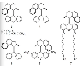
More recently, this first rotary molecular motor have been redesigned in order to improve its performances and, specifically, to lower the barriers to the rate-determining thermal steps. With this purpose a second-generation of this kind of motors was devel-oped [7]; in this new kind of systems the unidirectional rotation can be achieved with a single stereogenic centre and it was observed that an increase of the size of atoms X and Y (fig. 3.1) increases the steric crowding in the fjord region, resulting in slower thermal rotation steps.

The passage from a six-membered ring to a five-membered ring in the lower half of the molecule (from structure 4 to structure 5 in figure 3.1) caused [9] an increase in rotation speed by a 108factor. The thermal helix inversion step of the fast molecular motor 5 has an half-life of 3.15 minutes at room temperature. The structure was also modified [10] with the result that motor 6 could be powered by visible light (436nm) instead of UV light. Finally, in motor 7, light driven unidirectional rotation of the rotor unit when the stator is tethered to the surface of gold nanoparticles was recently demonstrated [8]. Furthermore, the motor was employed as a four-state light-triggered switch to construct a molecular gearbox in which the state of the switch controls the thermal rotation of an appended aromatic moiety [11].

(32)

Figure 3.1: - Molecular structures of the second generation of photochemical rotary molecular motors. Image credits [7-8].

This kind of molecular motors can be, in future, used as molecular switch in many di↵erent application such as nanocomputers and nanoswitches; Their functioning prin-ciple has been incorporated into a prototype nanocar [12]. Finally, the ability of certain second generation rotary molecular motors to act as an asymmetric catalyst has also been demonstrated [13-14].

It is hence very important, and interesting, to fully understand the functioning principles and the physics of these molecules; understanding completely the thermo-dynamic of the helix inversion process can be in future useful in order to predict the di↵erent properties of the molecules and assist the scientists during the design of these kind of molecules.

Under the hood: The physics of Molecular Motors dynamic

How is possible to describe the dynamic of a rotary molecular motor? To answer this question we have to start from the environment in which the molecular motor lives; molecular motors typically operates in solution; every molecule of the solvent, with its thermal fluctuations, collides to the molecules which are in it and exerts a force on them. In the simplest case this force will result in the well known Brownian Motion

(33)

phenomenon. In the simplest case the Brownian motion relates particle which are com-pletely free to move and will results in a comcom-pletely random motion of them. In the case of a molecular motor, the particle are not completely free to move; the system ”lives” inside a potential energy profile; the result is a biased Brownian Motion and in this case, a molecular motor can also be named as brownian motor. In this phenomena the movement of the solvent molecules will drive the molecular motor in his movement toward equilibrium. In order to correctly model these systems we need a proper phys-ical background which has to start from the definition of Brownian motion.

Brownian Motion

Brownian motion is the random motion of particles suspended in a fluid resulting from their collision with the quickly moving atoms or molecules composing it (the fluid). The term ”Brownian motion” can also refer to the mathematical model used to describe such random movements, which is often called a particle theory [15]. This transport phenomenon took this name after the botanist Robert Brown, in 1827, while looking through a microscope at particles found in pollen grains in water, noted that the par-ticles moved through the water but was not able to determine the mechanisms that caused this motion. A concrete description of this interesting phenomena arrived in 1905, when Albert Einstein published a paper [16] that explained in precise detail how the motion that Brown had observed was a result of the pollen being moved by indi-vidual water molecules thermal fluctuations around their position. This explanation of Brownian motion served as definitive confirmation that atoms and molecules actually exist, and was further verified experimentally by the Nobel prize Jean Perrin [17]. The direction of the force of atomic bombardment is constantly changing, and at di↵erent times the particle is hit more on one side than another, leading to the seemingly random nature of the motion.

The Einstein’s theory of the Brownian motion in composed of two main parts; in the first a formulation of a di↵usion equation for Brownian particles, in which the di↵usion coefficient is related to the mean squared displacement of a Brownian particle, is made. In the second part the di↵usion coefficient is related to measurable physical quantities.

(34)

The first part of Einstein’s argument was to determine how far a Brownian particle travels in a given time interval.[16] Classical mechanics was unable to determine this distance because of the enormous number of bombardments a Brownian particle will undergo, roughly of the order of 1021 collisions per second.[18] Thus Einstein was led to consider the collective motion of Brownian particles; he showed that if ⇢(x, t) is the density of Brownian particles at point x at time t, then ⇢ will obey the Fick’s equation for di↵usion:

@⇢ @t = D

@2_⇢

@x2 (3.1)

where D is mass di↵usivity.

Assuming that all the particles, at time t0= 0, starts from the origin, the di↵usion

equation has the solution

⇢(x, t) = _p⇢0 4⇡Dte

x2

4Dt (3.2)

With this expression is possible to calculate directly the moments; the first moment is seem to vanish, meaning that the Brownian particle is equally likely to move to the left as it is to move to the right. The second moment is, however, non vanishing, and reads

¯

x2_{= 2Dt} _(3.3)

This expression means that the mean squared displacement in terms of the time elapsed and the di↵usivity. From this expression Einstein argued that the displacement of a Brownian particle is not proportional to the elapsed time, but rather to its square root. His argument is based on a conceptual switch from the ensemble of Brownian particles to the single Brownian particle, with this approach we can start to speak in terms of probability distribution of the Brownian particles. Obtained the expression 3.2 the determination of the di↵usion coefficient was central to Einstein’s theory; he determined this quantity in terms of molecular qualities as follows.

(35)

The Maxwell-Boltzmann distribution for the configuration of Brownian particles which are in a field of force F (x) (i.e. the gravitational field of earth) reads

⇢ = ⇢0e U (3.4)

If the force is constant, as would be true for the gravity which acts on particles, the potential energy is

U = F x (3.5)

Now the velocity of a particle that is in equilibrium under the action of the applied force and viscosity is given by the Stoke’s law:

v = F

6⇡⌘a (3.6)

We can also derive the current density of the particles, i.e. the number of particles crossing unit area in unit time which is

j = ⇢F

6⇡⌘a (3.7)

For a normal di↵usion process, the particles cannot be created or destroyed, which means that the flux into one space region must be the sum of particles flux flowing out of the surrounding regions. The can be summarized mathematically by the continuity equation:

@⇢

@t +rJ = 0 (3.8)

Combining eqs. 3.1 with 3.8 and integrate over x will give us

D@⇢ @x =

⇢F

6⇡⌘a (3.9)

and, combining eqs. 3.5 with 3.4 we get 1 ⇢ @⇢ @x = F kBT (3.10)

(36)

So, comparing equations 3.9 and 3.10 we obtain the definition for the di↵usion coefficient

D = kBT

6⇡⌘a (3.11)

in which T is the temperature, ⌘ is the viscosity of the liquid and a is the size of the particle. This equation means that large particles would di↵use more gradually than smaller molecules, making them easier to measure.

Experimental observation confirmed the numerical accuracy of Einstein’s theory. We understand di↵usion in terms of the movements of the individual particles, and can calculate the di↵usion coefficient of a molecule if we know its size or, viceversa, we can calculate the size of the molecule after experimental determination of the di↵usion coefficient. Thus, Einstein connected the macroscopic process of di↵usion with the mi-croscopic concept of thermal motion of individual molecules.

The aforementioned discussion holds true only for pure brownian motion; for a molecular motor, we need to think in terms of biased brownian motion. The molecule of the solvent will acts on the moving parts of the molecular motor as they does for a free Brownian particle but, since the motor works inside an anisotropic energetic environment, this would bias the motion of it caused by the solvent hits. The result would essentially be di↵usion of a particle whose net motion is strongly biased in one direction.

Biased Brownian Motion

Before we go deeper into the physics of Brownian motor and to study their basic prin-ciples we have to introduce a more general principle that runs Brownian motion: the biased Brownian motion. The basic idea is simple: a system which isn’t in thermal equi-librium tends toward equiequi-librium. If such a system lives in an asymmetric world, then moving towards equilibrium will usually also involve a movement in space. To keep the system moving, we need to perpetually keep it away from thermal equilibrium, which costs energy - this is the energy that drives the motion. This result is reachable in many ways such as fluctuating temperature, chemical reactions, periodically turning

(37)

on and o↵ asymmetric potentials or by forcing periodic a Brownian particle.

Figure 3.2: - This figure illustrates how Brownian particles, which was initially located at the point x0 (lower picture), spreads out when the potential is turned o↵. When the

potential is turned on again, most particles are captured again in the attraction point x0,

but also exists a probability to find them in the point x0+ L (hatched area). This will

result in a net current to the particles to the right.

All these processes can be described by inducing some external potential U(x) in the system. In the case where our periodic potential U(x) has exactly one minimum and maximum per period L as in figure 3.2, it is quite obvious that if the local minimum is closer to its adjacent maximum to the right (fig. 3.2) a positive particle current, ˙x > 0, will arise. So in devices based on Brownian motion, net transport occurs by a combination of di↵usion and deterministic motion induced by proper applied force fields.

In order to describe these phenomena we start introducing the Langevin theory which will lead us to the stochastic di↵erential equations and, finally, the Fokker-Planck equation. Langevin began by simply writing down the equation of motion for the Brownian particle according to Newton’s law under the assumption that the particle experiences two forces:

(38)

(i) a fluctuating force that changes direction and magnitude frequently compared to any other time scale of the system and averages to zero over time;

(ii) a viscous drag force that always slows the motions induced by the fluctuation term.

This equation, named Langevin motion equation, according to Newton’s second law of motion, is md 2_x(t) dt2 = ⇣ dx(t) dt + F (x, t) + f (t)stoch (3.12) in which F (x, t) represents some optional external force. The friction term ⇣ ˙x is assumed to be governed by Stoke’s law which states that the frictional force decelerating a spherical particle of radius a is

⇣ ˙x = 6⇡⌘a ˙x (3.13)

where ⌘ is the viscosity of the surrounding medium. For the fluctuating part f (t)stoch

the following assumptions are made:

(i) f (t)stoch is independent of the space (x), (ii) f (t)stoch varies extremely rapidly

compared to the variation of x(t), (iii) the statistical average over an ensemble of par-ticles, f (t)stoch= 0, since f (t)stochis so irregular.

From solutions to the Langevin equations is possible to retrieve a large number of informations about the described system; however this is fully true in case of purely microscopic considerations. If one wants to to study the properties and the dynamic of bigger systems (systems composed of_{⇡N particles) limitations of this model and of} its classic approach becomes evident. If we want to fully describe the time evolution of whole a macroscopic environment we have to solve the Langevin’s motion equation for every particle which is part of such a system and it is also necessary to know, for every particle, initial position and velocity. Doing this is not impossible but requires a huge amount of time and calculation power; is better, in order to describe successfully complex problems, to change approach; is thus convenient to take the helpful and the advantages of the statistical mechanics.

(39)

A stochastic approach: the Fokker-Planck equation

A more efficient approach to the biased Brownian motion problem is given by the Fokker-Planck equation (FPE ) which is just an equation of motion for the distribution function of fluctuating macroscopic variables. The di↵usion equation 3.1 for the distri-bution function of an assembly of free Brownian particles is a simple example of such a equation. This equation is useful not only for the description of the Brownian motion but it can be used to explain a lot of di↵erent problems such as mathematics or financial problems [19]; is possible to say that the main use of the Fokker-Planck equation is as an approximate description for any Markov process in which the individual jumps are small. In its simplest and more general form the FPE reads:

@ @tP (x, t) = @ @x(D1(x, t)P (x, t)) + @2 @x2(D2(x, t)P (x, t)) (3.14)

where P (x, t) indicates the probability density distribution of the stochastic variable being studied (it can be the position or velocity of a population of Brownian particles) and the parameter D1and D2, which can be dependent by space, time, both or simple

constants, are, respectively, the drift and di↵usion coefficients; they will takes di↵erent forms depending of which is the case being solved. It is also of very interest to notice that, in the special case of a zero drift coefficient the FPE reduces simply to the well known di↵usion equation. Mathematically, the FPE is partial di↵erential equation of the second order, of parabolic kind; it is also knowed as forward Kolmogorov relation. Solutions to the FPE can be achieved analytically only in special cases. A formal anal-ogy of the Fokker–Planck equation with the Schroedinger equation allows the use of advanced operator techniques known from quantum mechanics for its solution in terms of eigenvalues and eigenfunctions for a restricted number of cases [19].

For the Brownian particle problem we can get the value of the drift coefficient out of Langevin equation [20] and the value of the di↵usion coefficient directly from Einstein’s considerations [16]. For the particular situation of a Brownian motor, which is the situation of a biased Brownian motion of a particle under the presence of a potential energy profile is possible to rewrite the FPE obtaining a particular form of it knowed as Klein-Kramer equation. This equation is a special case of the Fokker-Planck

(40)

equation and it is a motion equation for a distribution function describing both position and velocity of a Brownian particle under the presence of an external force and it reads.

@P (x, v, t) @t =  _@ @x + @ @v ✓ v F (x) m ◆ + kBT m @2 @v2 P (x, v, t) (3.15)

in which is the viscous drag constant, m is the mass of the particle, T is the solvent temperature, kB is the Boltzmann constant and, finally, F (x) = mf0(x) is

the external force result of the potential energy profile. Is thus possible to a↵ord [21] that the Brownian motor lives in a situation in which the inertial e↵ects are negligible, a situation knowed as low Reynold numbers or high viscous coefficients situation. An equation, particular case of the eq. 3.15, which have been written for this special cases, is the Smoluchowski equation:

@P (x, t) @t = 1 m  _@ @xF (x) + kBT @2 @x2 P (x, t) (3.16)

This last equation, which describes the dynamic, in terms of position, of a prob-ability distribution is the one of interest for us in order to achieve the first target of our research work. From solutions of it is hence possible to retrieve a huge quantity of informations about the dynamic and the physics of the system which is studied as we will see in the next chapter when we apply this mathematical approach to the dynamic of the motion of a rotary molecular motor; we will also apply the most recent compu-tational chemistry aids in order to extract the potential energy path where the motor exploit his action.

References

[1] Kay, E. R., Leigh, D. and Zerbetto, F. (2007). Synthetic molecular motors and mechanical machines. Angewandte Chemie (International ed. in English) (Vol. 46, pp. 72–191).

[2] M. Schliwa, G. Woehlke, Nature 2003, 422, 759. doi:10.1038/ NATURE01601

(41)

[4] T. Ross Kelly, Harshani De Silva and Richard A. Silva (1999). Unidirectional rotary motion in a molecular system. Nature 401, 150-152. doi:10.1038/43639;

[5] J. Vicario, M. Walko, A. Meetsma and Ben L. Feringa, Fine Tuning of the Ro-tary Motion by Structural Modification in Light-Driven Unidirectional Molecular Mo-tors, Journal of the American Chemical Society 2006 128 (15), 5127-5135

[6] N. Koumura, R. W. J. Zijlstra, R. A. van Delden, N. Harada, B. L. Feringa, Nature 1999, 401, 152. doi:10.1038/43646

[7] N. Koumura, E. M. Geertsema, A. Meetsma, B. L. Feringa, J. Am. Chem. Soc. 2002, 124, 5037. doi:10.1021/JA012499I

[8] R. A. van Delden, M. K. J. ter Wiel, M. M. Pollard, J. Vicario, N. Koumura, B. L. Feringa, Nature 2005, 437, 1337. doi: 10.1038/NATURE04127

[9] J. Vicario, A. Meetsma, B. L. Feringa, Chem. Commun. 2005, 5910. doi:10.1039/B507264F

[10] R. A. van Delden, N. Koumura, A. Schoevaars, A. Meetsma, B. L. Feringa, Org. Biomol. Chem. 2003, 1, 33. doi:10.1039/B209378B

[11] M. K. J. ter Wiel, R. A. van Delden, A. Meetsma, B. L. Feringa, Org. Biomol. Chem. 2005, 3, 4071. doi:10.1039/B510641A

[12] En Route to a Motorized Nanocar Jean-Fran¸cois Morin, Yasuhiro Shirai, and James M. Tour Org. Lett.; 2006, 8, 1713-1716.

[13] Dynamic Control of Chiral Space in a Catalytic Asymmetric Reaction Us-ing a Molecular Motor Science 18 March 2011: Vol. 331 no. 6023 pp. 1429-1432 doi:10.1126/science.1199844

(42)

[14] Heat and Light Switch a Chiral Catalyst and Its Products Science 18 March 2011: Vol. 331 no. 6023 pp. 1395-1396 doi:10.1126/science.1203272

[15] M¨orters, Peter; Peres, Yuval (25 May 2008). Brownian Motion

[16] Einstein, Albert (1905). ” Über die von der molekularkinetischen Theorie der Wärme geforderte Bewegung von in ruhenden Flüssigkeiten suspendierten Teilchen”.

Annalen der Physik 17 (8): 549–560. Bibcode:1905AnP...322..549E. doi:10.1002/andp.19053220806.

[17] Perrin J. B. (1916) Atoms

[18] Chandresekhar, S. Stochastic problems in physics and astronomy. Rev. Mod-ern Phys. 15, (1943). 1–89.

[19] Risken H., The Fokker-Planck Equation: Methods of Solutions and Applica-tions, 2nd edition, Springer Series in Synergetics, Springer, ISBN 3-540-61530-X

[20] W.T. Co↵ey, Yu. P. Kalmykov, J. T. Waldron, The Langevin equation, World Scientific, Singapore, 1998

(43)

4

Rotary molecular motors

dynamic revealed

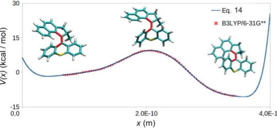
In the previous chapter we have described what the molecular motors are and how their physics can be explained using the Fokker-Planck equation. In this section the first main target of our work is presented; we will provide a general framework that makes possible the estimation of time-dependent properties of a stochastic system moving far from equilibrium like the motion of an artificial molecular motor. The process is investigated and discussed in general terms of non-equilibrium thermodynamics. The approach is simple and can be exploited to gain insight into the dynamics of any molecular-level machine. As a case study, we examine the dynamics of an artificial molecular rotary motor, similar to the inversion of a helix, which drives the rotor from a metastable state to equilibrium as we seen in chapter 3. The energy path that the motor walks was obtained from the results of atomistic calculations. The changes in time of the motor entropy, internal energy, free energy, net-exerted force by the motor, and the efficiency of its unidirectional motion are given, starting from the solution of the Smoulochowski’s equation (solutions obtained with the FEM computational method). The amount of available energy converted to heat due to the net-motion is rather low revealing that the motion is mainly subject to randomness.

(44)

Theoretical framework

As mentioned in chapter 3 the dynamic of a system (an artificial molecular motor) evolving from a far from equilibrium situation and subject to the environmental fluc-tuations that acts on it will be done using the Smoluchowski equation

@P (x, x0; t) @t = D @2_{P (x, x} 0; t) @x2 + 1 @ @x ⇢_{@V (x)} @x (P (x, x0; t)) (4.1) where P (x, x0; t) is the probability density function related to the position of a

par-ticle population, D is the di↵usion coefficient, V (x) is the potential energy profile of the path where the system lives, and is the friction coefficient of the solvent. According to Stoke’s law, for spherical objects = 2d⇡⌘r, with ⌘ the temperature dependent viscosity coefficient of the medium, r the radius of the rotor, and d the dimensionality of the motion.

Combining the continuity equation (4.2) @P (x, x0; t)

@t +

@J(x, t)

@x = 0 (4.2)

with equation 4.1, the resulting flux density (or probability current) in units of (s 1) reads:

J(x, t) = D@P (x, x0; t) @x

1 @V (x)

@x P (x, x0; t) (4.3)

According to Gibb’s definition, the entropy production of the rotor is

S(t) = kB

Z L 0

P (x, x0; t)ln(P (x, x0; t))dx (4.4)

The time derivative of the eq. 4.4 in terms of the probability density, the flux, and the conservative force, F (x) = @xV (x), reads [1]

dS dt = kB Z L 0 J2(x, t) DP (x, x0; t)dx kB D Z L 0 F (x)J(x, t)dx (4.5)

The second part at the right hand side of eq. 4.5, kB

D

RL

0 F (x)J(x, t)dx, multiplied

(45)

change of the entropy of the medium. The entire entropy production rate (entropy of the rotor plus environment) is [1]

dStot dt = kB Z L 0 J2(x, t) DP (x, x0; t) dx 0 (4.6)

The inequality of eq. 4.6 becomes an equality only when the system is at equilibrium and the total flux is zero (detailed balance).

In terms of the probability density function the change of the internal energy reads:

U = Z L

0

V (x)_{{(P (x, x}0; t) P (x0; 0)} dx (4.7)

and the heat dissipated by the particle up to time teq takes the form

Qh_d= kBT D Z teq 0 Z L 0 F (x)J(x, t)dxdt (4.8)

and the change in the free energy, combining eqs.4.4 and 4.7, reads

F = Z L 0 V (x)_{{(P (x, x}0; t) P (x0; 0)} dx+ kBT Z L 0 P (x, x0; t)ln(P (x, x0; t))dx kBT Z L 0 P (x0, 0)ln(P (x0, 0))dx (4.9)

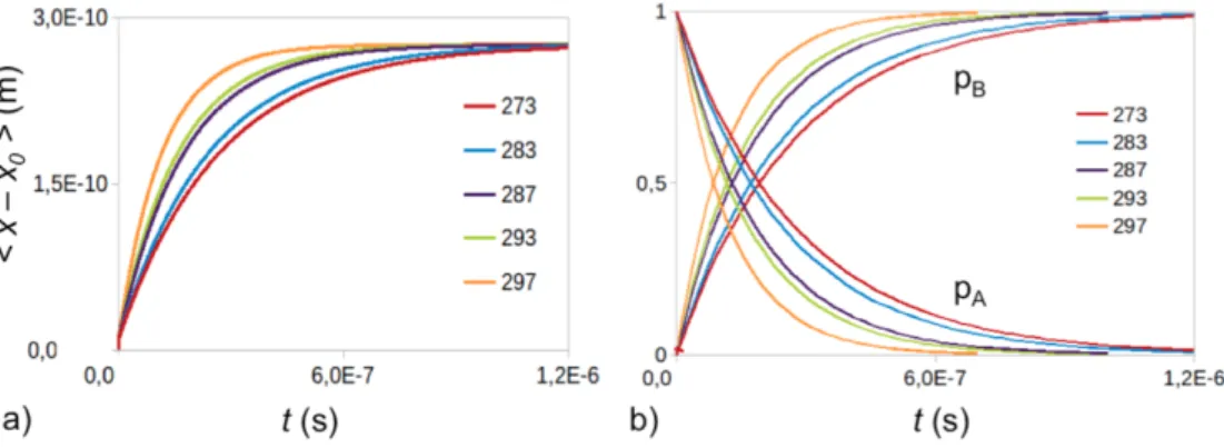
where teq is the time needed to the system to reach equilibrium. This time can be

provided by the analysis of the mean displacement, which connects the initial and the final position of the particle at time t.

< x x0> (t) =

Z L 0

(x x0)P (x, x0; t)dx (4.10)

The equilibration time, teq, is reached when the mean displacement reacher a plateau

and its value is ”almost equal” to the distance between the two minima. The time derivative of the mean displacement provides additional information, namely, the mean velocity of the motion of the motor

v(t) = d < x x0> (t)

dt =

Z L 0

J(x, t)dx (4.11)

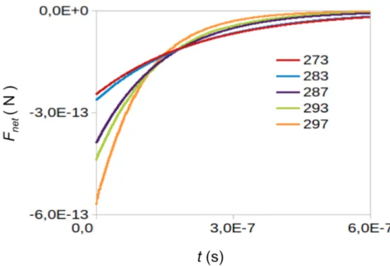
When the mean velocity di↵ers from zero, a net-motion occurs and part of the avail-able energy is converted into heat. The work done by the motor up to time t is given as

(46)

the path integral of the net-fore exerted by the motor over the trajectory followed by the system, W =Rx(teq)

x(0) Fnet(x(t))dx(t), where we approximate Fnet(t) = Ff r(t) = v(t).

Since the system evolves from a situation which is far from equilibrium, the dissipation-fluctuation theorem does not hold for this case a di↵erent approximation is necessary. Taking into account that two competitive minima are present in the bistable potential and that the force is a vector dependent quantity, we write for the net-exerted force by the rotor due to the ith minimum [3]

F_neti (t) = Z t 0 (Z xi,m b F (x)p(x, t0)dx Z xb xi,m F (x)p(x, t0)dx ) dt0 (4.12) in which p(x, t) is the probability distribution and NOT the probability density function, b is the position of the boundary (to the left or to the right of the minimum), xi,mis the position of the minimum, and xb is the position of the energy barrier. The

total net-force exerted by the particle will be

Fnet(t) = Fnetdeep(t) Fnetshal(t) (4.13)

where the superscripts deep and shal indicates the deeper and shallower minimum, respectively. The total work done by the rotor until equilibrium is reached reads

W = Z teq

0

Fnet(t)v(t)dt (4.14)

Coupling eqs. 4.9 and 4.14 we can obtain the efficiency of the motor which, in percent, reads

✏ = W

F ⇥ 100 (4.15)

All the quantities here listed can be easily obtained, for a given potential energy profile and a given solvent, after numerical solutions of eq. 4.1;

• the change of the internal energy, eq. 4.7, • the change in the free energy, eq. 4.9, • the mean displacement, eq. 4.10,

(47)

• the net exerted force by the particle, eq. 4.12, • the work done by the particle, eq. 4.14, and • the efficiency of the motor, eq. 4.15.

In the next sections we will see in detail which is the studied molecular motors, its properties and how we start from experimental evidences in order to construct a proper potential energy profile; we will also see how we solved the Smoluchowski equation which describes the evolution of the system.

The chosen molecular motor

The studied molecular motor is described in the article [4]; in that paper a particular kind of rotary molecular motor is synthesized and presented; it is composed by two main parts: a rotor and a stator which are linked by a -C=C- bond which can be photo-isomerized (355nm for 9 seconds) driving the molecule out of equilibrium (un-stable situation). The more (un-stable situation will be naturally recovered through a helix inversion process. If we consider that the photo-isomerization occurs instantaneously ( t_{⇡ 0), the recovery of the equilibrium will require a time which can varies with the} temperature, the solvent and the substituents presents on the molecule. An example of this kind of molecule is showed in the Figure 4.1.

In the latter figure the mechanism that underlie the rotation of the motor is ex-plained; this mechanism is simply to understand talking in terms of potential energy surfaces (PES ); the di↵erent relative positions of the stator and the rotor lies on di↵er-ent points, which are at di↵erdi↵er-ent energies, on a potdi↵er-ential energy surface as explained in the Figure 4.2.

(48)

Figure 4.2: - Mechanism that underlie the relative rotation of the rotor and the stator in a synthetic rotational molecular motor, Reprinted with permission from Ref [5]. Copyright 2008 American Chemical Society.

For our study we selected the most simple rotary molecular motor which is described in the already cited article; this molecule 4.3 is a cyclopentane based molecular motors in which all the substituents on the six term aromatic carbon rings are hydrogen. Finally there is an S atom at the bottom of the structure.

Figure 4.3: - Structure of the molecule which have been studied in the present work; the red bonds are the ones around which the two parts of the molecule rotates.

The group that has synthesised these molecule have demonstrate that cyclopentane-based molecular rotary motors, which display even less steric hindrance can accomplish