AN INTEGRATED APPROACH TO ACCIDENT ANALYSIS IN PWR

(1)

Autore:

Eugenio Coscarelli

Firma__________

Relatori:

Prof. Ing. Francesco D’Auria Firma__________

Ing. Giorgio M. Galassi Firma__________

Ing. Alessandro Del Nevo Firma__________

AN INTEGRATED APPROACH TO

ACCIDENT ANALYSIS IN PWR

Anno 2013

UNIVERSITÀ DI PISA

Scuola di Dottorato in Ingegneria “Leonardo da Vinci”

Corso di Dottorato di Ricerca in

SICUREZZA NUCLEARE E INDUSTRIALE

(2)

(3)

(4)

When you measure what you are speaking about, and express it in numbers, you know something about it; but when you cannot measure it, when you cannot not express it in numbers, your knowledge is of a meager and unsatisfactory kind: it may be the beginning of

knowledge, but you have scarcely, in your thoughts, advanced to the stage of the science.

William Thomson, Lord Kelvin, from Popular Lectures and Addresses, 1891-1894

(5)

RINGRAZIAMENTI

Vorrei ringraziare quanti hanno permesso con la loro fattiva collaborazione ed il loro prezioso aiuto la realizzazione di questo lavoro. In primo luogo vorrei ringraziare il Prof. Ing. Francesco D’Auria per aver messo a disposizione il suo enorme bagaglio di esperienza e competenza tecnica nel campo della termoidraulica contribuendo in questo modo alla definizione degli obiettivi di questa ricerca.

Vorrei ringraziare i miei relatori, il Dott. Ing Giorgio Galassi ed il Dott. Ing. Alessandro Del Nevo che mi hanno supportato (ma soprattutto sopportato) in questo percorso, fornendomi preziosi suggerimenti attraverso i quali sono riuscito a superare le non poche difficoltà che sono emerse durante l’attività di ricerca. Un ringraziamento particolare lo vorrei rivolgere ad un guru della termoidraulica, il Dott. Herbert Staedtke con il quale ho avuto interessanti e profondi scambi di idee che hanno illuminato il mio cammino nel complesso ed affascinante mondo della fluidodinamica bifase.

Ringrazio il Prof. Walter Ambrosini e Juan Carlos Ferreri che stimo per la profonda competenza tecnica, ma soprattutto perché ognuno di loro ha rappresentato un punto di riferimento per la mia attività di ricerca.

Vorrei ringraziare i miei più cari amici che mi sono stati vicini in questo lungo periodo di studio: Andrea, Cesare e Paola, Giancarlo e Alessandro. Un ringraziamento particolare va all’Ing. Daniele Martelli compagno di mille esami e collega dello stesso corso di dottorato.

Un profondo ringraziamento va ai miei genitori: Ada e Antonio per la loro incrollabile fiducia che hanno sempre risposto in me. Ringrazio anche i mie due nipoti Angelo e Antonio, le mie sorelle Silvana e Filomena, i miei cognati Alessandro e Carmine, per essere stati sempre presenti.

Un ringraziamento particolarmente affettuoso va, infine a mia moglie Rosa che mi è stata vicina nei momenti più difficili di questo lavoro sostenendomi materialmente e moralmente.

(6)

(7)

ABSTRACT

The purpose of the present doctoral research is to provide a contribute to the TH-SYS codes assessment for nuclear reactor applications, and particularly for the predictive analysis of PWR transient behavior, such as MSLB accident scenario, in which strong coolant flow asymmetries and multi-dimensional turbulent mixing effects strongly influence two relevant safety issues: recriticality and PTS.

The contribution consists in proposing and developing of an integrated analytical approach for TH-SYS code (TRACE-V5) assessment in relation to the investigation of the coolant transient flow processes in the reactor coolant system. The developed approach is focused on set up a methodology able to assess the accuracy of the numerical predictions based on the use of reliable experimental database that covers all relevant thermal hydraulic processes observed to occur simultaneously at system and component phenomenological levels during a selected accident scenario in a PWR system. To achieve this goal the first phase was to perform an independent assessment through the formulation of an independent assessment matrix for two classes of tests (basic test and integral effect test). The aim was to evaluate the capabilities of the code and models in reproducing the relevant thermal-hydraulic phenomena which characterize the simulated experiments. The second phase has concerned the development of the integrated methodology by defining a specific transient scenario important for PWR system safety (namely MSLB). Once the specific scenario has been identified, the methodology was oriented to define the relevant phenomena and processes that drive the system response. After the definition of all phenomena and interactions during the selected scenario, a corresponding process for establishing a test matrix was developed. The construction of the test matrix was carried out identifying a set of tests performed in integral and separate effects tests facilities achieved in a complementary way. Finally, the suitability of code in predicting the results of the complementary tests was obtained splitting the quantification of the accuracy in two phases. The first phase concerned the evaluation of the accuracy in a integral sense that is assess the code results at the system level (analysis of the overall thermal hydraulic response of the PWR system) against experimental data of the integral test performed in PKL-III facility. The second phase was oriented to measure the code discrepancies focusing the attention to the component level phenomena identified in the PWR system during the accident scenario under investigation and not experimental captured by the integral test. This last phase is connected, from the experimental point of view, with the tests carried out in the ROCOM test facility. In this way it is possible to cover experimentally the overall spectrum of phenomena expected to occur during the MSLB transient and assess the computational results using the same code (TRACE-V5 TH-SYS code) to simulate both tests: integral and separate effects tests.

Therefore, the methodology addresses also the issue of the validation of the 3-dimensional modules existing as an option in the codes like TRACE-V5 in simulating complex multi-dimensional flow patterns, such as mixing flow present in the RPV during the transient scenario (MSLB).

(8)

In view of the methodology goals, the work is supported by code validation and application results obtained in the frame of OECD/NEA CSNI PKL-2 project. It consists of an experimental program of eight tests (G series) carried out in integral test facility. The third test, identified as G3.1, has been selected for the application of the integrated approach, since the results of this PKL test, which is oriented PWR system behavior, also provide the boundary conditions for complementary tests in the ROCOM facility on mixing cold and hot water in the RPV downcomer as well as in the lower plenum and for determining the fluid state at the core inlet. Within the proposed approach, the relevant modelling issues are identified and discussed, so as to point out the main capabilities and limitations in the present state-of-the-art tools and methods.

(9)

INDEX

RINGRAZIAMENTI ... v

ABSTRACT ... vii

INDEX ... ix

ABBREVIATIONS ... xv

LIST OF FIGURES ... xvii

LIST OF TABLES ... xxviii

1 INTRODUCTION ... 1

1.1. Objectives of the research ... 1

1.2. Framework ... 2

1.3. Description of the performed activity ... 2

1.4. Structure of the document ... 4

2 DETERMINISTIC SAFETY ANALYSIS AND BEST ESTIMATE

APPROACH ... 5

2.1. Framework ... 5

2.2. Deterministic safety analysis ... 6

2.2.1. Conservative approach ... 6

2.2.2. Best estimate approach ... 7

3 STATE OF THE ART IN THE APPLICATION OF TH-SYS

CODES TO NRS ... 8

3.1. History and current status of TH-SYS codes ... 8

3.2. Assessment strategy: Verification and validation (V&V) ... 14

3.3. Needs and challenges in nuclear thermal hydraulics ... 16

3.4. Overview of EU projects connected to TH-SYS ... 21

4 METHODOLOGY FOR INDEPENDENT ASSESSMENT OF

TH-SYS CODES ... 23

4.1. Overview of independent Assessment approach ... 23

4.1.1. Independent assessment matrix ... 25

(10)

4.2.1. Description of the facility and experiment ... 27

4.2.1.1. PKL-III test facility description (configuration) ... 27

4.2.1.2. PKL-III test F4.1 ... 35

4.2.1.2.1. Objectives of the test F4.1 ... 35

4.2.1.2.2. Outline of the test F4.1 ... 35

4.2.1.3. PKL-III test G7.1 ... 39

4.2.1.3.1. Objectives of the test G7.1 ... 39

4.2.1.3.2. Configuration of the facility, boundary and initial conditions of the experiment ... 40

4.2.1.3.3. Outline of the test G7.1 ... 40

4.2.2. TRACE-V5 nodalization development for PKL facility ... 45

4.2.2.1. Features of TRACE-V5 nodalization for simulating the test F4.1 .. ... 45

4.2.2.2. Features of TRACE-V5 nodalization for simulating the test G7.1 . ... 46

4.2.3. Analytical study of heat transfer mechanisms under shutdown

system conditions (PKL test F4.1) ... 49

4.2.3.1. Analysis of the post test results ... 49

4.2.4. Investigation of TH-SYS code performance for SBLOCA

phenomenology (PKL test G7.1) ... 65

4.2.4.1. Analysis of the post test results ... 65

4.3. Gravity dominant test: water faucet problem ... 80

4.3.1. Description of the water faucet problem ... 81

4.3.2. Analytical solution ... 82

4.3.3. Numerical solution ... 84

4.4. Outcomes of the independent assessment process ... 87

5 DEVELOPMENT OF AN INTEGRATED APPROACH FOR

ACCIDENT ANALYSIS AND CODE QUALIFICATION (TRACE

CODE) ... 90

5.1. Outline of the methodology ... 90

5.2. Selection of the accident scenario: Main Steam Line Break

(MSLB) ... 93

5.3. Phenomena identification ... 95

(11)

5.5. Establishing of the test matrix ... 98

5.6. Accuracy evaluation for complementary tests ... 100

6 APPLICATION OF IA TO PKL-2/ROCOM EXPERIMENTS ... 103

6.1. PKL-2 Project PKL-III Test G3.1 ... 103

6.1.1. Objectives of Test G3.1 ... 103

6.1.2. Configuration of the facility, boundary and initial conditions of

the experiment ... 104

6.1.2.1. PKL Test G3.1 break component and characterization ... 104

6.1.3. Outline of the PKL-III G3.1 experiment ... 104

6.1.4. Selected parameters for code assessment ... 106

6.2. Adopted nodalization for simulating the PKL-III G3.1 test .... 117

6.3. Analysis of the post-test calculation results ... 120

6.3.1. Evaluation of steady state results ... 120

6.3.2. Comparison and evaluation of reference results ... 123

6.3.2.1. Qualitative accuracy evaluation ... 123

6.3.2.1.1. Table of resulting sequence of main events ... 123

6.3.2.1.2. Selected time trends ... 124

6.3.2.1.3. Qualitative accuracy evaluation of the RTA ... 126

6.3.3. Quantitative accuracy evaluation by the Fast Fourier Transform

Based Method ... 126

6.4. Buoyancy/convective driven flow mixing experiments

(ROCOM tests) ... 145

6.5. Description of the ROCOM test facility ... 145

6.6. ROCOM instrumentation ... 150

6.6.1. Measurement principles ... 150

6.6.2. Location of the wire-mesh sensors in the facility ... 150

6.7. Outline of the ROCOM/PKL tests ... 152

6.7.1. Scaling assumptions ... 153

6.7.2. The ROCOM test 1.1 ... 154

6.7.2.1. Objectives of the test ... 154

6.7.2.2. Initial and Boundary conditions ... 154

(12)

6.7.4. ROCOM test 2.2 ... 157

6.8. TRACE-V5 code Simulation ... 158

6.8.1. Thermodynamic considerations ... 162

6.8.2. Simulation of the test 1.1 ... 162

6.8.2.1. Analysis of the results: experiment/simulation temporal comparison ... 163

6.8.2.1.1. Pseudo local analysis ... 163

6.8.2.1.2. Averaging analysis ... 164

6.8.2.2. Analysis of the results: experiment/simulation spatial comparison ... 164

6.8.3. Simulation of the test 1.2 ... 180

6.8.3.2. Analysis of the results: experiment/simulation spatial comparison ... 182

6.8.4. Simulation of the test 2.2 ... 196

6.8.5. Quantitative accuracy: application of the FFTBM to the

simulated ROCOM tests ... 210

6.8.6. Effect of the noding scheme on the numerical simulation... 216

6.9. Concluding remarks on the IA application to the PKL/ROCOM

test ... 219

7 CONCLUSIONS ... 223

(13)

APPENDIX A.

CODES USED WITHIN THE RESEARCH:

TRACE-V5 code

232 A.1.

Overview of TRACE ... 232

A.2.

Governing equations ... 233

A.2.1. Interfacial drag force ... 235

A.2.2. Wall drag force ... 236

A.2.3. Wall condensation and boiling ... 236

A.2.4. Heat conduction ... 236

A.3.

Physical phenomena considered ... 236

A.4.

Numerical approach ... 237

A.5.

References to APPENDIX A ... 238

APPENDIX B.

DESCRIPTION OF THE PKL TRACE

NODALIZATION ... 240

B.1.

Description of the TRACE-V5 nodalization ... 240

B.2.

Verification of the volumes in the nodalization ... 245

B.3 References to APPENDIX B ... 255

APPENDIX C.

ASSESSMENT OF PRESSURE DROPS OF PKL

NODALIZATION ... 256

C.1.

Verification and set up of the pressure drops ... 256

C.2.

References to APPENDIX C ... 269

APPENDIX D.

DESCRIPTION OF THE ROCOM TRACE

NODALIZATION ... 271

APPENDIX E.

QUANTIFICATION OF THE ACCURACY: THE

FFTBM AND THE APPLICATION ... 277

E.1.

Description of the Fast Fourier Transform Based Method. 277

E.1.1. Background ... 277

E.1.2. Method development ... 278

E.1.3. Methodology implementation ... 282

E.1.3.1. Sampling frequency ... 282

E.1.3.2. Number of points ... 282

(14)

E.1.3.4. Choice of the weights ... 283

E.1.3.5. FFT package ... 285

E.1.4. Application of the method to sample curves ... 286

(15)

ABBREVIATIONS

3-D Three Dimensional

AM Accident Management

BE Best Estimate

BEPU Best Estimate Plus Uncertainty

BC Boundary Conditions

BIC Boundary Initial Conditions

CET Core Exit Temperature/Component Effect Test

CFD Computational Fluid Dynamics

CFR Code of Federal Regulation

CHF Critical Heat Flux

CL Cold Leg

COMBO Continuous Measurement of Boron Concentration

CPh Conditioning Phase

CSNI Committee on the Safety of Nuclear Installations

CSP Core Support Plate

DBA Design Basis Accident

DIMNP Department of Mechanical, Nuclear and Production Engineering of University of Pisa, Italy

ECCS Emergency Core Cooling System

FA Fuel Assembly

FC Fuel Channel

FFT Fast Fourier Transform

FFTBM Fast Fourier Transform Based Method

FP Fission product

FSAR Final Safety Analysis Report

GRNSPG San Piero a Grado Nuclear Research Group

GT Guide Tube

HL Hot Leg

I & C Instrumentation and control IAEA International Atomic Energy Agency IAM Independent Assessment Matrix

IC Initial Conditions

ITF Integral Test Facility

LB-LOCA Large Break LOCA

LOCA Loss of Coolant Accident

LS Loop Seal

MSL Main Steam Line

MSLB Main Steam Line Break

MSRCV Main Steam Relieve Control Valve

NEA Nuclear Energy Agency

NPP Nuclear Power Plant

OECD Organization for the Economic Cooperation and Development

PCT Peak Cladding Temperature

Ph.W. Phenomenological Window

(16)

PRZ Pressurizer

PS Primary Side

PWR Pressurized Water Reactor

RBV Rod Bundle Vessel

RC Reflux Condensation

RCS Reactor Coolant System

RCL Reactor Coolant Loop

RPV Reactor Pressure Vessel

SBLOCA Small Break LOCA

SETF Separate Effect Test Facility SETS Stability Enhancing Two Step

SG Steam Generator

SoT Start of Transient

SPNC Single Phase Natural Circulation

SS Secondary Side

SYS System

TH Thermal-Hydraulic

THS Thermal-Hydraulics Safety

TMF Turbulent Mixing Flow

TPNC Two Phase Natural Circulation UNIPI University of Pisa

(17)

LIST OF FIGURES

Figure 1 – Flow chard of PhD performed research activity ... 3

Figure 2 – Spectrum of SET, CET and IET facilities. ... 5

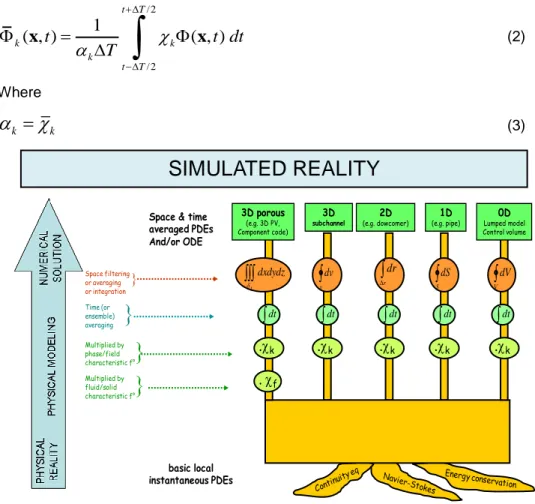
Figure 3 – The successive steps for establishing and solving thermal-hydraulic equations. ... 10

Figure 4 – Attributes and feature requested for a TH-SYS code... 13

Figure 5 – Flow diagram for verification and validation of a system code [27]. ... 15

Figure 6 – Flow diagram for verification of a system code. ... 15

Figure 7 – Flow diagram for validation of a system code ... 16

Figure 8 – Outline of the code assessment process ... 23

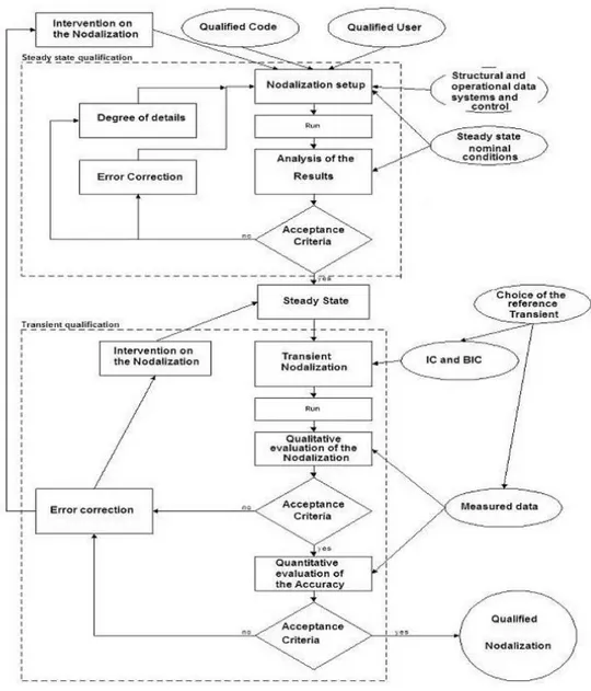
Figure 9 – Flow diagram of the nodalization process ... 25

Figure 10 – PKL III experiment F4.1 RUN 1: boron concentration measurement instruments locations ... 33

Figure 11 – PKL III test facility and RCS-dimensions ... 34

Figure 12 – PKL-III F4.1 RUN 1: measured trends of loop average mass flow rate and non-dimensional residual mass inventory ... 38

Figure 15 – Break line: hot leg 1 to separator vessel ... 43

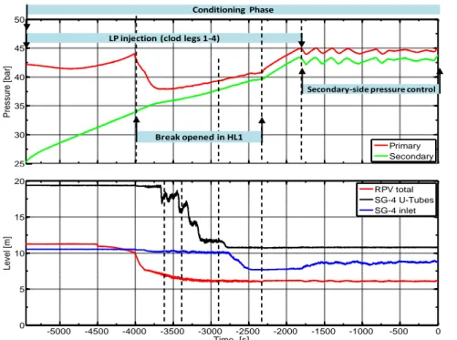
Figure 16 – PKL Test G7.1: pressure and liquid levels trends during the test phase conditioning phase ... 44

Figure 17 – PKL Test G7.1 test phase: pressure and liquid levels trends during the test phase ... 44

Figure 18 – PKL Test G7.1 test phase: pressure and peak cladding/core exit temperature trends during the test phase ... 45

Figure 19 – TRACE-V5 nodalization of the PKL III integral test facility ... 47

Figure 20 – Azimuthal and radial nodalization of the core region ... 48

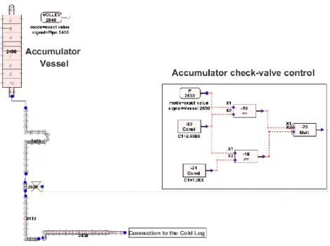
Figure 21 – TRACE-V5 Nodalization of the accumulator and cold leg connection 48 Figure 22 – TRACE-V5 Nodalization of the break line ... 49

Figure 23 – PKL III test F4.1 RUN 1, posttest results: loop 1 SG outlet mass flow rate trends (0 – 70230 s) ... 55

Figure 24 – PKL III test F4.1 RUN 1, posttest results: loop 2 SG outlet mass flow rate trends (0 – 70230 s) ... 55

Figure 25 – PKL Test F4.1, posttest results: loop 3 SG outlet mass flow rate trends (0 – 70230 s) ... 56

(18)

Figure 26 – PKL III test F4.1 RUN 1, posttest results: loop 4 SG outlet mass flow rate trends (0 – 70230 s) ... 56 Figure 27 – PKL III test F4.1 RUN 1, posttest results: UP pressure trends ... 57 Figure 28 – PKL Test F4.1, posttest results: SG-1 pressure trends ... 57 Figure 29 – PKL III test F4.1 RUN 1, posttest results: LP coolant temperature trends ... 58 Figure 30 – PKL III test F4.1 RUN 1, posttest results: core collapsed level ... 58 Figure 31 – PKL III test F4.1 RUN 1, posttest results: primary side total mass (without PRZ) ... 59 Figure 32 – PKL III test F4.1 RUN 1, posttest results: differential temperature SG-1 inlet/outlet ... 59 Figure 33 – PKL III test F4.1 RUN 1, posttest results: differential temperature SG-4 inlet/outlet ... 60 Figure 34 – PKL III test F4.1 RUN 1, posttest results: DP inlet outlet SG-1 primary side ... 60 Figure 35 – PKL III test F4.1 RUN 1, posttest results: DP inlet outlet SG-4 primary side ... 61 Figure 36 – PKL III test F4.1 RUN 1, posttest results: boron concentration in CL-1 ... 61 Figure 37 – PKL III test F4.1 RUN 1, posttest results: boron concentration in CL-3 ... 62 Figure 38 – PKL III test F4.1 RUN 1, posttest results: SG -1 U-tube ascending side collapsed levels ... 62 Figure 39 – PKL III test F4.1 RUN 1, posttest results: SG -3 U-tube ascending side collapsed levels ... 63 Figure 40 – PKL III test F4.1 RUN 1, posttest results: SG -1 U-tube descending side collapsed levels ... 63 Figure 41 – PKL III test F4.1 RUN 1, posttest results: SG -3 U-tube descending side collapsed levels ... 64 Figure 42 – PKL III test F4.1 RUN 1, posttest results: loop seal 1 descending side collapsed level ... 64 Figure 43 – PKL Test G7.1, posttest results: hot leg 1 break mass flow rate ... 70 Figure 44 – PKL Test G7.1, posttest results: hot leg 1 collapsed level (vertical) (-600 – 3300 s) ... 70 Figure 45 – PKL Test G7.1, posttest results: differential temperature SG 1 inlet/outlet ... 71 Figure 46 – PKL Test G7.1 , posttest results: differential temperature SG 4 inlet/outlet ... 71

(19)

Figure 47 – PKL Test G7.1, posttest results: UP and SG-1 pressure trends (-500 – 1550 s) ... 72 Figure 48 – PKL Test G7.1, posttest results: UP and SG-1 pressure trends (-500 – 3300 s) ... 72 Figure 49 – PKL Test G7.1, posttest results: MSL 1 nozzle mass flow rate trends (secondary side depressurization) ... 73 Figure 50 – PKL Test G7.1, posttest results: MSL 3 nozzle mass flow rate trends (secondary side depressurization) ... 73 Figure 51 – PKL Test G7.1, posttest results: SG-1 riser collapsed level (-100 – 3300 s) ... 74 Figure 52 – PKL Test G7.1, posttest results: SG-1 riser collapsed level (-100 – 3300 s) ... 74 Figure 53 – PKL Test G7.1, posttest results: DP DC vessel inlet /RPV outlet (-600 – 3300 s) ... 75 Figure 54 – PKL Test G7.1, posttest results: hot legs collapsed level (horizontal) (-600 – 3300 s) ... 75 Figure 55 – PKL Test G7.1, posttest results: core collapsed level (-600 – 3300 s) 76 Figure 56 – PKL Test G7.1, posttest results: DC pipe collapsed level (-600 – 3300 s) ... 76 Figure 57 – PKL Test G7.1, posttest results: loop seal 1 SG side collapsed level 77 Figure 58 – PKL Test G7.1, posttest results: loop seal 4 SG side collapsed level 77 Figure 59 – PKL Test G7.1, posttest results: CET trends ... 78 Figure 60 – PKL Test G7.1, posttest results: PCT trends (500 – 3300 s) ... 78 Figure 61 – PKL Test G7.1, posttest results: Core fluid temperature trends in subchannels at core level ME7 ... 79 Figure 62 – PKL Test G7.1, posttest results: total mass flow rate injected by ACCs in CL-1 – CL-4 ... 79 Figure 63 – PKL Test G7.1, posttest results: total mass flow rate injected by LPISs in CL-1 - CL-4 ... 80 Figure 64 – Schematic of the time evolution of liquid Column ... 81 Figure 65 – analytical solution: void fraction and liquid velocity trends ... 84 Figure 66 – numerical simulation of the discontinuity wave propagation and velocity profile at three different time points ... 85 Figure 67 – numerical simulation of the discontinuity wave propagation and velocity profile in the case of grid refinement (100 cells) ... 85 Figure 68 – numerical simulation of the discontinuity wave propagation and velocity profile in the case of grid refinement (384 cells) ... 86

(20)

Figure 69 – effects of the grid refinement (500 cells) on the numerical error

(dispersion error, high wave number oscillations) ... 86

Figure 70 – void fraction distribution at different time: comparison of analytical solution with TRACE-V5 results ... 87

Figure 71 – Phenomenology of the PTS: breaking down the phenomena identification and separation in different phenomenological levels (system and component/local) ... 92

Figure 72 – Scaling strategy to perform complementary test ... 93

Figure 73 – Complementary test: initial and boundary conditions provided to SET rig (ROCOM) from IET facility (PKL) ... 98

Figure 74 – AREVA NP PKL-III facility: elevations. ... 110

Figure 75 – AREVA NP PKL-III facility: elevations. ... 111

Figure 76 – AREVA NP PKL-III facility: steam generator ... 112

Figure 77 – AREVA NP PKL-III facility: Test G3.1 steam line break device. ... 112

Figure 78 – AREVA NP PKL-III facility: pressurizer relief line ... 113

Figure 79 – PKL-III pressure drop characterization: DP vs. length at mass flow rate equal to 0.8 kg/s ... 113

Figure 80 – AREVA NP PKL-III facility characterization: DP vs. length at mass flow rate equal to 25 kg/s ... 114

Figure 81 – AREVA NP PKL-III facility characterization: heat losses vs. temperature ... 114

Figure 82 – OECD/NEA/CSNI PKL-2 Project Test G3.1: boundary conditions: MCP coastdown dimensionless velocity vs. time ... 115

Figure 83 – OECD/NEA/CSNI PKL-2 Project Test G3.1: pressures in PRZ, UP, SGs, BRK line downstream the orifice and PRZ level. ... 115

Figure 84 – OECD/NEA/CSNI PKL-2 Project Test G3.1: coolant temperatures in PRZ. ... 115

Figure 85 – OECD/NEA/CSNI PKL-2 Project Test G3.1: coolant temperatures in RPV and RCS. ... 116

Figure 86 – OECD/NEA/CSNI PKL-2 Project Test G3.1mass flow rates in the loops. ... 116

Figure 87 – OECD/NEA/CSNI PKL-2 Project Test G3.1: levels in SG-1, SG-2 and BRK mass flow rate. ... 116

Figure 88 – OECD/NEA/CSNI PKL-2 Project Test G3.1: mass flow rates injected by HPIS in CL-1 and CL-4 ... 117

Figure 89 – TRACE model of the main steam line and break orifice ... 118

(21)

Figure 91 – PKL Test G3.1: primary system pressure drop vs. length ... 123

Figure 92 – PKL Test G3.1, posttest results: PRZ pressure trends ... 133

Figure 93 – PKL Test G3.1, posttest results: SG-1 pressure trends ... 133

Figure 94 – PKL Test G3.1, posttest results: SG-4 pressure trends ... 134

Figure 95 – PKL Test G3.1, posttest results: LP coolant temperature trends ... 134

Figure 96 – PKL Test G3.1, posttest results: UP coolant temperature trends ... 135

Figure 97 – PKL Test G3.1, posttest results: CL 1 SG outlet coolant temperature trends ... 135

Figure 98 – PKL Test G3.1, posttest results: CL 4 SG outlet coolant temperature trends ... 136

Figure 99 – PKL Test G3.1, posttest results: differential temperature SG 1 inlet/outlet ... 136

Figure 100 – PKL Test G3.1, posttest results: loop 1 SG outlet mass flow rate trends (-100 – 4410 s) ... 137

Figure 104 – PKL Test G3.1, posttest results: MSL 1 BRK nozzle mass flow rate trends (-100 – 4410 s) ... 139

Figure 105 – PKL Test G3.1, posttest results: DP DC vessel inlet /RPV outlet (100 – 4410 s) ... 139

Figure 106 – PKL Test G3.1, posttest results: DP inlet/outlet SG 1 (0 – 4410 s) 140 Figure 107 – PKL Test G3.1, posttest results: DP inlet/outlet SG 4 (0 – 4410 s) 140 Figure 108 – PKL Test G3.1, posttest results: PRZ collapsed level (-100 – 4410) ... 141

Figure 109 – PKL Test G3.1, posttest results: SG-1 riser collapsed level (-100 – 4410) ... 141

Figure 110 – PKL Test G3.1, posttest results: SG-2 riser collapsed level (-100 – 4410) ... 142

Figure 111 – PKL Test G3.1, posttest results: integral BRK mass flow trends (-100 – 1100 s). ... 142

Figure 112 – PKL Test G3.1, posttest results: hottest cladding temperature at 5.62m from RPV bottom (-100 – 4500 s). ... 143

(22)

Figure 113 – PKL Test G3.1, benchmark posttest FFTBM application: quantitative accuracy evaluation of the results – from 0 up to 1030 s. ... 143 Figure 114 – PKL Test G3.1, benchmark posttest FFTBM application: quantitative accuracy evaluation of the results – overall transient ... 144 Figure 115 – The Fast Fourier Transform Based Method (FFTBM): evaluation of the quality of the result of the total average amplitude. ... 144 Figure 116 – Model of the reactor vessel, vertical section ... 146 Figure 117 – Model of the reactor vessel, cross section in the nozzle region ... 147 Figure 118 – Sieve drum in the lower plenum of the ROCOM test facility ... 147 Figure 119 – Model of the lower core support plate ... 148 Figure 120 – Schematic of the ROCOM test facility with numbering of the loops and positions of different wire-mesh sensors in the loops ... 149 Figure 121 – Core inlet mesh sensor: general view (a), electrode (b). ... 151 Figure 122 – Core wire mesh sensors position into the downcomer and at the core inlet. ... 151 Figure 123 – Wire mesh sensor for pipes. ... 151 Figure 124 – Measurement loop temperature in the PKL test G3.1. ... 152 Figure 125 – Configuration before starting the test (a), Configuration of the test facility during run. ... 155 Figure 126 – Schematic of the ROCOM test facility with ECC injection nozzles . 157 Figure 127 – Measured loop mass flow rates in the ROCOM Test 2.2 ... 158 Figure 128 – Spatial resolution of the computational and experimental downcomer sensors ... 160 Figure 129 – Spatial resolution of the computational and experimental downcomer sensors ... 161 Figure 130 – ROCOM experiment 1.1 reference results: temperatures trends at the downcomer top layer ... 166 Figure 131 – ROCOM experiment 1.1 reference results: temperatures trends at the downcomer middle layer ... 167 Figure 132 – ROCOM experiment 1.1 reference results: temperatures trends at the downcomer bottom layer ... 168 Figure 133 – Snapshots of the temperature distribution in the downcomer (outer plane) at five different time points in tests 1.1 (experimental (a), calculated (b)) . 169 Figure 134 – ROCOM experiment 1.1 reference results: temperatures trends at the core inlet first radial ring, all azimuthal sectors. ... 170 Figure 135 – ROCOM experiment 1.1 reference results: temperatures trends at the core inlet second radial ring, all azimuthal sectors. ... 171

(23)

Figure 136 – ROCOM experiment 1.1 reference results: temperatures trends at the core inlet third radial ring, all azimuthal sectors. ... 172 Figure 137 – ROCOM experiment 1.1 reference results: temperatures trends at the core inlet fourth radial ring, all azimuthal sectors. ... 173 Figure 138 – ROCOM experiment 1.1: snapshots of the temperature distribution in the core inlet at six different time points in tests 1.1. (part 1 of 2) (experimental (a), calculated (b)) ... 174 Figure 139 – ROCOM experiment 1.1: snapshots of the temperature distribution in the core inlet at six different time points in tests 1.1. (part 2 of 2) (experimental (a), calculated (b)) ... 175 Figure 140 – ROCOM experiment 1.1 averaged temperature evolution inside the DC ... 176 Figure 141 – ROCOM experiment 1.1: averaged temperature evolution at the core inlet ... 176

Figure 142 – ROCOM experiment 1.1: experimental (a) and simulated (b)

temperature time averaged value in the DC outer plane (time averaging interval: t = 73 s to t = 83 s) ... 177 Figure 143 – ROCOM experiment 1.1: experimental (a) and simulated (b) temperature time averaged value at the core inlet (time averaging interval: t = 73 s to t = 83 s) ... 178 Figure 144 – ROCOM experiment 1.1: downcomer time averaged temperature horizontal cut ... 179 Figure 145 – ROCOM experiment 1.1: downcomer time averaged temperature vertical cut ... 179 Figure 146 – ROCOM experiment 1.2 reference results: temperatures trends at the downcomer top layer ... 183 Figure 147 – ROCOM experiment 1.2 reference results: temperatures trends at the downcomer middle layer ... 184 Figure 148 – ROCOM experiment 1.2 reference results: temperatures trends at the downcomer bottom layer ... 185 Figure 149 – ROCOM experiment 1.2: snapshots of the temperature distribution in the downcomer (outer plane) at five different time points in tests 1.2 (experimental (a), calculated (b)) ... 186 Figure 150 – ROCOM experiment 1.2 reference results: temperatures trends at the core inlet first radial ring, all azimuthal sectors ... 187 Figure 151 – ROCOM experiment 1.2 reference results: temperatures trends at the core inlet second radial ring, all azimuthal sectors ... 188 Figure 152 – ROCOM experiment 1.2 reference results: temperatures trends at the core inlet third radial ring, all azimuthal sectors ... 189

(24)

Figure 153 – ROCOM experiment 1.2 reference results: temperatures trends at the core inlet fourth radial ring, all azimuthal sectors ... 190 Figure 154 – ROCOM experiment 1.2: snapshots of the temperature distribution in the core inlet at six different time points (part 1 of 2) (experimental (a), calculated (b)) ... 191 Figure 155 – ROCOM experiment 1.2: snapshots of the temperature distribution in the core inlet at six different time points (part 2 of 2) (experimental (a), calculated (b)) ... 192

Figure 156 – ROCOM experiment 1.2: averaged temperature evolution inside the

DC ... 193 Figure 157 – ROCOM experiment 1.2: averaged temperature evolution at the core inlet ... 193 Figure 158 – ROCOM experiment 1.1: experimental (a) and simulated (b) temperature time averaged value in the DC outer plane (time averaging interval: t = 60 s to t = 70 s) ... 194 Figure 159 – ROCOM experiment 1.2: experimental (a) and simulated (b) temperature time averaged value at the core inlet (time averaging interval: t = 60 s to t = 70 s) ... 195 Figure 160 – ROCOM experiment 2.2 reference results: temperatures trends at the downcomer top layer ... 198 Figure 161 – ROCOM experiment 2.2 reference results: temperatures trends at the downcomer middle layer ... 199 Figure 162 – ROCOM experiment 2.2 reference results: temperatures trends at the downcomer bottom layer ... 200 Figure 163 – ROCOM experiment 2.2: snapshots of the temperature distribution in the downcomer (experimental (a), TRACE-V5 results (b)) at different time points (t = 0 s is related to the start of the flow in loop 1) ... 201 Figure 164 – Snapshots of the experimental temperature distribution in the downcomer (outer plane) at three different time points (t= 50; 65; 80 s) in tests 1.1 and 2.2 ... 202 Figure 165 – Snapshots of the simulated temperature distribution in the downcomer (outer plane)at three different time points (t= 50; 65; 80 s) in tests 1.1 and 2.2 ... 203 Figure 166 – ROCOM experiment 1.2 reference results: temperatures trends at the core inlet first radial ring, all azimuthal sectors ... 204 Figure 167 – ROCOM experiment 1.2 reference results: temperatures trends at the core inlet second radial ring, all azimuthal sectors ... 205 Figure 168 – ROCOM experiment 1.2 reference results: temperatures trends at the core inlet third radial ring, all azimuthal sectors ... 206

(25)

Figure 169 – ROCOM experiment 1.2 reference results: temperatures trends at the core inlet fourth radial ring, all azimuthal sectors ... 207 Figure 170 – ROCOM experiment 2.2: snapshot of the temperature distribution in the core inlet plane at t = 50 s in the (experimental results (a), TRACE-V5 results (b) ... 208

Figure 171 – ROCOM experiment 2.2: averaged temperature evolution inside the

DC ... 209 Figure 172 – ROCOM experiment 2.2: averaged temperature evolution at the core inlet ... 209 Figure 173 – ROCOM experiment 1.1: application of the FFTBM to the temperature distribution at the core inlet ... 212 Figure 174 – ROCOM experiment 1.2: application of the FFTBM to the temperature distribution at the core inlet ... 212 Figure 175 – ROCOM experiment 2.2: application of the FFTBM to the temperature distribution at the core inlet ... 213 Figure 176 – ROCOM experiment 1.1: application of the FFTBM to the spatial averaged temperature inside the DC and at the core inlet ... 214 Figure 177 – ROCOM experiment 1.2: application of the FFTBM to the spatial averaged temperature inside the DC and at the core inlet ... 214 Figure 178 – ROCOM experiment 2.2: application of the FFTBM to the spatial averaged temperature inside the DC and at the core inlet ... 215 Figure 179 – ROCOM experiment 1.1, noding sensitivity analysis: DC average temperature trends ... 217 Figure 180 – ROCOM experiment 1.1, noding sensitivity analysis: DC average temperature trends ... 217

Figure 181 – ROCOM experiment 1.1, noding sensitivity analysis: FFTBM

accuracy quantification (DC average temperature trends) ... 218

Figure 182 – ROCOM experiment 1.1, noding sensitivity analysis: FFTBM

accuracy quantification (DC average temperature trends) ... 218 Figure 183 – TRACE nodalization: RBV scheme ... 242 Figure 184 – TRACE nodalization: core ... 242 Figure 185 – TRACE nodalization: DC vessel and DC-UH bypass ... 243 Figure 186 – TRACE nodalization: SG secondary side ... 243 Figure 187 – TRACE nodalization: loop 2, SG 2 primary and secondary side, PRZ system... 244 Figure 188 – Volume vs Elevation: Rod Bundle Vessel (without Reflector Gap) . 246 Figure 189 – Volume vs Elevation: RPV Downcomer ... 247

(26)

Figure 190 – Volume vs Elevation: Loop 1 (SG Outlet, Pump Seal, Reactor Coolant Pump, Cold Leg Horizontal Section) ... 248 Figure 191 – Volume vs Elevation: hot leg and SG inlet (Loop 1) ... 248 Figure 192 – Volume vs Elevation: Steam Generator primary side (Loop 1) ... 249 Figure 193 – Volume vs Elevation: Pressurizer... 250 Figure 194 – Volume vs Elevation: Steam Generator Secondary Side ... 251 Figure 195 – Volume vs Elevation: Reflector Gap ... 252 Figure 196 – Head losses measurement system sketch: identification of the zones ... 258 Figure 197 – PKL III facility nodalization qualification: low range, loop mass flow equal from 0.80 to 3.60 kg/s ΔP vs. squared mass flow: MCP zone (MST 199) . 259 Figure 198 – PKL III facility nodalization qualification: low range, loop mass flow equal from 0.80 to 3.60 kg/s ΔP vs. squared mass flow: CL zone (MST 208) ... 259 Figure 199 – PKL III facility nodalization qualification: low range, loop mass flow equal from 0.80 to 3.60 kg/s ΔP vs. squared mass flow: RPV zone (MST 172) .. 260 Figure 200 – PKL III facility nodalization qualification: low range, loop mass flow equal from 0.80 to 3.60 kg/s ΔP vs. squared mass flow: HL zone (MST 173) ... 260 Figure 201 – PKL III facility nodalization qualification: low range, loop mass flow equal from 0.80 to 3.60 kg/s ΔP vs. squared mass flow: SG UT zone (MST 181) ... 261 Figure 202 – PKL III facility nodalization qualification: low range, loop mass flow equal from 0.80 to 3.60 kg/s ΔP vs. squared mass flow: LS zone (MST 190) ... 261 Figure 203 – PKL III facility nodalization qualification: low range, loop mass flow equal from 0.80 to 3.60 kg/s ΔP vs. squared mass flow: BV zone (MST 198) ... 262 Figure 204 – PKL III facility nodalization qualification: low range, loop mass flow equal from 0.80 to 3.60 kg/s ΔP vs. squared mass flow: DC vessel (MST 165) .. 262 Figure 205 – PKL III facility nodalization qualification: low range, loop mass flow equal from 0.80 to 3.60 kg/s ΔP vs. squared mass flow: DC tube (MST 50) ... 263 Figure 206 – PKL III facility nodalization qualification: low range, loop mass flow equal from 0.80 to 3.60 kg/s ΔP vs. squared mass flow: LP zone (MST 236) ... 263 Figure 207 – PKL III facility nodalization qualification: low range, loop mass flow equal from 0.80 to 3.60 kg/s ΔP vs. squared mass flow: core zone (MST 42) .... 264 Figure 208 – PKL III facility nodalization qualification: low range, loop mass flow equal from 5.00 to 25.02 kg/s ΔP vs. squared mass flow: UP zone (MST 44) .... 264 Figure 209 – PKL III facility nodalization qualification: ΔP vs length curve, Loop mass flow equal to 0.80 kg/s ... 265 Figure 210 – PKL III facility nodalization qualification: ΔP vs length curve, Loop mass flow equal to 1.20 kg/s ... 265

(27)

Figure 211 – PKL III facility nodalization qualification: ΔP vs length curve, Loop mass flow equal to 1.60 kg/s ... 266 Figure 212 – PKL III facility nodalization qualification: ΔP vs length curve, Loop mass flow equal to 2.00 kg/s ... 266 Figure 213 – PKL III facility nodalization qualification: ΔP vs length curve, Loop mass flow equal to 2.40 kg/s ... 267 Figure 214 – PKL III facility nodalization qualification: ΔP vs length curve, Loop mass flow equal to 2.80 kg/s ... 267 Figure 215 – PKL III facility nodalization qualification: ΔP vs length curve, Loop mass flow equal to 3.20 kg/s ... 268 Figure 216 – PKL III facility nodalization qualification: ΔP vs length curve, Loop mass flow equal to 3.60 kg/s ... 268 Figure 217 – definition of the 3-D fluid domain in the computational cells ... 273 Figure 218 – Volume porosity distribution in the TRACE-V5 vessel model ... 273 Figure 219 – ROCOM nodalization sketch: top view ... 274 Figure 220 – ROCOM nodalization sketch: front view ... 275 Figure 221 – Sample Fourier Transform representation ... 278 Figure 222 – Sample Problem 1: considered experimental and calculated cirves ... 287 Figure 223 – Accuracy evaluation using FFTBM: graphical representation of functions (experimental, calculated and error) in time domain ... 289 Figure 224 – Accuracy evaluation using FFTBM: spectrum of the experimental function ... 289 Figure 225 – Accuracy evaluation using FFTBM: spectrum of the calculated function ... 290 Figure 226 – Accuracy evaluation using FFTBM: spectrum of the error function 290

(28)

LIST OF TABLES

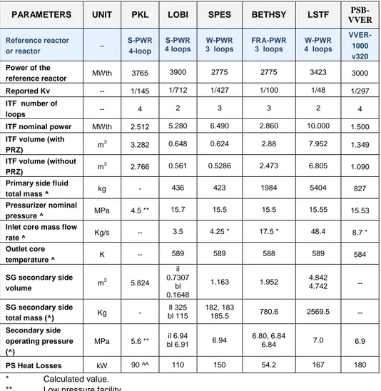
Table 1 – Independent assessment matrix... 27 Table 2 – AREVA NP PKL III versus LOBI, SPES, BETHSY, LSTF facilities and KRSKO NPP: hardware data of steam generators ... 31 Table 3 – AREVA NP PKL III versus LOBI, SPES, BETHSY, LSTF and PSB-VVER facilities: main scaling characteristics. ... 32 Table 4 – PKL III Test F4.1: relevant initial and boundary conditions ... 36 Table 5 – PKL III facility configuration ... 36 Table 6 – PKL III test F4.1 RUN 1: phenomenological analysis ... 37 Table 7 – OECD/NEA/CSNI PKL-2 Project, Test G7 1: facility configuration ... 42 Table 8 – OECD/NEA/CSNI PKL-2 Project, Test G7 1: relevant initial and boundary conditions at start of both conditioning phase and test phase... 43

Table 9 – PKL III test F4.1 RUN 1, TRACE-V5p2: comparison between measured and calculated relevant initial and boundary conditions. ... 53 Table 10 – PKL III test F4.1 RUN 1: summary of results obtained by application of FFTBM (reference calculation) – overall transient. ... 54 Table 11 – PKL III Test G7 1, posttest results: resulting sequence of main events67 Table 12 – PKL Test G7.1 posttest: steady state results ... 68 Table 13 – PKL Test G7.1 posttest: summary of results obtained by application of FFTBM (reference calculation): (0 ─ 3300 s) ... 69 Table 14 – BICs for the water faucet problem ... 82 Table 15 – Key phenomena/processes relevant for the MSLB. (part 1 of 2) ... 95 Table 16 – Key phenomena/processes relevant for the MSLB (part 2 of 2) ... 96 Table 17 – Cross reference matrix for MSLB in PWR systems... 102 Table 18 – OECD/NEA/CSNI PKL-2 Project, Test G3.1: facility configuration. ... 107 Table 19 – OECD/NEA/CSNI PKL-2 Project, Test G3.1: relevant initial and boundary conditions. ... 107 Table 20 – OECD/NEA/CSNI PKL-2 Project, Test G3.1: ... 108

Table 21 – OECD/NEA/CSNI PKL-2 Project, Test G3.1: phenomenological

windows and resulting sequence of main events (part 1 of 2) ... 109

Table 22 – OECD/NEA/CSNI PKL-2 Project, Test G3.1: phenomenological

windows and resulting sequence of main events (part 2 of 2) ... 110 Table 23 – PKL Test G3.1 posttest: steady state results (part 1 of 3) ... 121 Table 24 – PKL Test G3.1 posttest: steady state results (part 2 of 3) ... 122

(29)

Table 25 – PKL Test G3.1 posttest: steady state results (part 3 of 3) ... 122 Table 26 – PKL Test G3.1, posttest results: resulting sequence of main events. 127 Table 27 – PKL Test G3.1, posttest results: qualitative accuracy evaluation on the basis of RTA (part 1 of 3)... 128 Table 28 – PKL Test G3.1, posttest results: qualitative accuracy evaluation on the basis of RTA (part 2 of 3)... 129 Table 29 – PKL Test G3.1, posttest results: qualitative accuracy evaluation on the

basis of RTA (part 3 of 3)... 130 Table 30 – PKL Test G3.1, posttest results: summary of results obtained by application of FFTBM – from 0 up to 1030 s ... 131 Table 31 – PKL Test G3.1, posttest results: summary of results obtained by application of FFTBM – overall transient ... 132 Table 32 – Some characteristics of ROCOM facility compared to those of a KONVOI reactor. ... 149 Table 33 – ROCOM test matrix ... 153 Table 34 – Conditions in PKL test G3.1 at t = 609 s (P = 3.8MPa) ... 154 Table 35 – Initial and Boundary conditions of ROCOM Test 1.1 ... 155 Table 36 –Conditions in PKL test G3.1 at t = 1500 s (P = 3.97MPa) ... 156 Table 37 – Initial and Boundary conditions of ROCOM Test 1.2 ... 156 Table 38 – Initial and Boundary conditions of ROCOM Test 2.2 ... 158 Table 39 – ROCOM experiment 1.1: boundary conditions of the TRACE-V5 model (P=3.8 MPa) ... 162 Table 40 – ROCOM experiment 1.1: adopted procedure ... 163 Table 41 – ROCOM experiment 1.2: boundary conditions of the TRACE-V5 model (P=3.97 MPa) ... 180 Table 42 – ROCOM experiment 1.2: adopted procedure ... 180 Table 43 – ROCOM experiment 2.2: adopted procedure ... 196 Table 44 – Results of accuracy quantification in the DC for selected calculations ... 213 Table 45 – Nodalization development ... 253 Table 46 – Characteristic of the nodalization geometry ... 254 Table 47 – PKL III facility nodalization qualification: Tests DRUV 1 2 boundary conditions and time sequence of the events ... 257 Table 48 – Volume porosity distribution in the CSP ... 272 Table 49 – Volume porosity distribution in the LP (subdivided in 3 axial mesh) .. 272

(30)

(31)

1 INTRODUCTION

Arguably no other field of engineering depends so strongly on the development and assessment of numerical simulation tools (like TH-SYS or CFD codes) as nuclear technology and especially nuclear safety. The applications of the numerical

process simulation in the framework of safety and licensing is mainly due to the

impracticability of executing full-scale safety related experiments and the absence of simplified scaling criteria for the important physical processes (occurring during the scenarios of interest) which would allow a direct transfer of results from small scale test facilities to the nuclear power plant. The main objective of developing numerical simulation tools (TRACE, RELAP5, CATHARE, etc.) was to replace the

evaluation model (EM) approach which includes the definition of a limited number

of worst case scenarios in combination with conservative assumption by

best-estimate (BE) methodologies. Best-best-estimate approach, aimed to provide a detailed

realistic description of postulated accident scenarios based on best-available modelling methodologies and numerical solution strategies, is the current strategy adopted in nuclear thermal hydraulic safety analysis. A consequence extensive experimental programs in scaled down integral and separate effect test facilities are conducted for solving open issues of current nuclear power plant designs, for demonstrating the technical feasibility of innovative designs, and for generating reference databases in order to support codes development and assessment [1]. Experimental data are fundamental for demonstrating the reliability of computer codes in simulating the behavior of a NPP during a postulated accident scenario: in general, this is a regulatory requirement [2].International efforts have been lavished to promote and organize activities aimed at increasing confidence in the validity and accuracy of analytical tools and demonstrating the competences of the involved institutions. Relevant examples of those activities are the ISP [3] under the aegis of the NEA/CSNI (the ISP-50 is currently ongoing and the draft report of the blind phase has been issued [4]), the ICSP sponsored by IAEA (e.g. the ICSP on MASLWR is currently ended [5]), but also analytical exercises carried out and documented in the framework of international groups connected with experimental programs in test facilities (e.g. Refs. [5], [6] and [8]).

1.1. Objectives of the research

The performed research activity is aimed at contributing to the assessment of TH-SYS codes in their application to issues related to the safety analysis of nuclear technology, in particular for the predictive analysis of complex transient two-phase flow and heat transfer conditions as expected to occur in Light Water Reactors (LWR) under accident and off-normal conditions. In this frame, this research is designed to approach new challenges and future needs in nuclear thermal-hydraulics which might arise from the simultaneous modelling of multi-dimensional effects which are always present in the full-size plant during an accident scenario. The fulfillment of this aspect will require the development of new strategies for the validation of 3-D prediction capability using experimental data that coming from

(32)

integral and separate effect tests carried out following an integrated approach (namely executed in a complementary way). In this way it is possible to reproduce at the scaled level the broad spectrum of phenomena featuring the specific accidental transient (system and component level) as well as to assess the TH-SYS codes toward a best estimate thermal hydraulic modeling.

1.2. Framework

The research has been carried out in the framework of the OECD/NEA CSNI PKL-2, http://www.nea.fr/jointproj/pkl.html, (2008-2012) and has thus profited of the availability of large experimental databases as well as of the connection to a wide number of internationally recognized experts in the fields of nuclear reactor safety and thermal-hydraulic and code development and assessment. The project is aimed at studying selected accident scenarios at system level, understanding the thermal hydraulic phenomena and processes occurring in pressurized water reactor design as well as validating and improving complex thermal-hydraulic system codes used in safety analysis. The experimental program consists of eight tests (G series), carried out in PKL-III facility by AREVA NP in Erlangen (Germany). It represents the scaled down layout of a 1300-MW PWR NPP (KWU-Siemens, Philippsburg NPP unit 2).

1.3. Description of the performed activity

The activity performed for fulfilling the objectives of the research is outlined in Figure 1. The steps below were executed to fulfill the following objectives:

 acquisition of expertise in the thermal hydraulic field, taking advantage from the participation in international activities;

 investigation of issue related to the use of TH-SYS codes and related methodologies;

 development of a methodology and related tools for accident analysis in PWR systems;

 qualification activities to support the reliability of the analyses;

 application of the methodology for predicting the phenomenology expected to occur during a MSLB scenario simulated in PKL-III/ROCOM test facilities.

The work is the result of the following TH-SYS code-related activities carried out within the San Piero a Grado Research Group (GRNSPG) of University of Pisa:

 TH-SYS code analyses for various purposes such as code assessment against integral and separate effect tests and investigation of the code numerical scheme capabilities through numerical tests;

 supporting nuclear reactor safety studies, etc.;

 participation in international meetings, workshops and events, being in contact with several internationally recognized experts.

(33)

Figure 1 – Flow chard of PhD performed research activity

Investigation of issue related to the use of TH-SYS codes in

nuclear safety Acquisition of expertise in

the thermal hydraulic field

Application of the methodology to the assessment of the TRACE-V5 code against MSLB scenario performed in

PKL-III and ROCOM test facilities

Transfer of results/knowledge

• Participation to international conferences and meetings (PRG/MB • Participation to expert groups (FONESYS

network)

• International projects (OECD/NEA/CSNI PKL-2 project) Benchmark on OECD/NEA/CSNI PKL-2 Project TEST G3.1 Mo d e l d e ve lo p me n t In d e p e n d e n t a sse ssme n

t Integral effect tests:

•Analytical study of heat transfer mechanisms under shutdown system conditions (PKL test F4.1)

•Investigation of TH-SYS code performance for SBLOCA phenomenology (PKL G7.1) Basic tests •Numerical test C o m p u ta ti o n a l a n d p o s t p ro c e s s in g to o ls d e v e lo p m e n t Verification Development of an integrated approach to accident analysis in

(34)

1.4. Structure of the document

The thesis is divided in seven chapters and five appendixes.

The Introduction contains the background information and the objective of the activity.

Chapter 2 describes the framework in which the methodology developed in this research, namely the best estimate deterministic safety approach.

Chapter 3 presents historical overview and the current state-of-the-art in the field of thermal-hydraulic numerical simulation related to nuclear technology and nuclear safety, with emphasis on various issues of TH-SYS codes.

Chapter 4 contains the description of the independent assessment approach for the TRACE-V5 code and nodalization assessment against experimental data from two PKL-III tests. The experimental facility is described, and the results obtained from the experiments are presented. In addition a basic numerical test has been selected to test the numerical characteristics of the algorithm implemented in the TRACE-V5 code.

Chapter 5 outlines the integrated analytical methodology to accident analysis in PWR systems.

Chapter 6 contains the results of the application of the integrated methodology for predicting the phenomenology characterizing the MSLB scenario throughout the comparison of the computational modelling results with the experimental results of the PKL-III/ROCOM complementary test (PKL test G3.1 and ROCOM test 1.1, 1.2 and 2.2)

(35)

2 DETERMINISTIC SAFETY ANALYSIS AND BEST ESTIMATE

APPROACH

2.1. Framework

Thermal hydraulic safety (THS) assessment represents the most relevant issue in the design and licensing of NPPs ensuring the acceptability of SM. The two main branches through which develops the THS process, are the deterministic safety analysis (DSA) and the probabilistic safety (PSA) analysis. The framework in which is developed the research activity is linked with DSA, the purpose of which is to address plant behavior under specific predetermined operational states and accident conditions. In regard to this objective the PWR thermal hydraulic safety evaluation and assessment, is closely related the development of more sophisticated analytical tools able to predict the time-space thermal-hydraulic conditions throughout the reactor coolant system.

Historically the emergency core cooling systems (ECCS) against LOCA scenario was one of the major topics of safety assessment for light water reactors established with the publication of the „Interim Acceptance Criteria (see [9]). This had as outcome the assessment of the thermal hydraulic safety analysis performed through the use of analytical and experimental methods, which in turn have resulted in various safety analysis codes and experimental facilities. Several integral and separate effect test facilities have been built and operated since 1960s (see Figure 2 in which is represented the spectrum of test facilities vs scale) aiming to provide useful information and experimental data on the thermal hydraulic behavior LWR under accident conditions and on the reliability of the TH-SYS code in performing accident analysis.

Figure 2 – Spectrum of SET, CET and IET facilities1 .

(36)

2.2. Deterministic safety analysis

Deterministic safety analysis is an important tool for confirming the adequacy and efficiency of provisions within the defense in depth concept for the safety of nuclear power plants (NPPs) [9]. Two different methodologies has been adopted to assess the deterministic thermal hydraulic safety analysis, namely the conservative approach and the best estimate approach. The concept of conservative methods was introduced in the early days of safety analysis to cover uncertainties that prevailed in the 1970s due to the limited capability of modelling and the limited knowledge of physical phenomena, and to simplify the thermal hydraulic analysis. The results obtained by this approach may be misleading (unrealistic behavior predicted, order of events changed) and level of conservatism is unknown. Therefore, there has been a move away from over-conservatism in safety analysis towards the application of so-called best estimate methodologies.

2.2.1. Conservative approach

The conservative approach has traditionally been used for the licensing analyses, being part of a NPP‟s commissioning activities and has to be submitted to and approved by the regulatory authority. In a traditional conservative analysis, both the assumed plant conditions and the physical models used are set conservatively. The reasoning is that such an approach would demonstrate that the calculated safety parameters are within the acceptance criteria and would ensure that no other transient of that category would exceed the acceptance criteria. However, in those analyses the safety margins obtained are expected to be conservatively large, as certain TH phenomena as well as certain plant and system features are not credited. Besides, it should be noted that the conservative approach does not provide any indications as to the true safety margins nor does it provide a true simulation of a specified scenario. For example, the assumption of a high core power level may lead to high levels of steam–water mixture in the core in the case of a postulated small break loss of coolant accident. Consequently, the calculated peak cladding temperature may not be conservative. As another example, the assumption that reduced interfacial shear between water and steam may lead to higher cladding temperatures in the upper core region, is conservative. However, this conservative assumption will lead to an optimistic estimate for the refilling/reflooding time, as it will appear that more water remains in the primary cooling system than is actually the case. In cases where a realistic analysis could demonstrate that important safety issues may be being masked, the conservative licensing calculations should be accompanied by a best estimate analysis, without

a) Cylindrical Core Test Facility. f)

Upper-Plenum Test

Facility. k) Loop for Blowdown Investigation. p)

Geradrohr Dampferzeuger Anlage. b) Counter current

flow limitation. g) Loss of Fluid Test. l) University of Maryland, College Park. q)

Steam-generator tube rupture. c) Slab Core Test

Facility. h)

Multiloop Integral Test Facility. m)

Full Length Emergency Cooling Heat Transfer-Separate Effects And Systems Effects Test.

r) Three Mile Island, Unit 2. d) Two dimensional. i) Rig of Safety

Assessment. n) Primarkreislaufe. e) Idaho National Engineering Laboratory. j) Simulatore PWR per Esperienze di Sicurezza.

(37)

an evaluation of the uncertainties, to ensure that important safety issues are not being concealed by the conservative analysis [10].

2.2.2. Best estimate approach

The best estimate approach is the actual trend of the NPP deterministic analysis [11]. The concept of best estimate is generally applied to the codes used in the analysis. However the best estimate approach concept has a broader meaning. It applies to the general framework of the analysis, and it involves not only the codes, but the kind of analyses to be performed, the approach to realize the models to be realized for the analyses, the input data including boundary and initial conditions also. The best estimate approach is not only connected with a calculation performed with a best estimate code. The result of the analysis is a best estimate evaluation, if all the aspects of the analysis (input data, systems models, results) are best estimate, in addition to the codes. As a consequence, the use of a best estimate code, assuming not best estimate data or systems model cannot be considered a best estimate analysis.

In the BE analyses, the TH phenomena are simulated as accurately as possible (according to present knowledge) and the safety margins obtained more closely reflect the real margins in the plant. This type of analyses also provides more realistic simulations of the NPP behavior during the course of the transient scenarios and can consequently reveal detailed system information that can be relevant for the understanding of TH phenomena interaction. If BE analyses are used for licensing purposes, they must be accompanied by uncertainty analyses to quantify the uncertainty of calculated parameters. The uncertainty includes contributions from simplifications introduced both into the governing equations and to the constitutive relationships and models, but also from using such models outside their original ranges of validity.