CIRTEN
CONSORZIO INTERUNIVERSITARIO
PER LA RICERCA TECNOLOGICA NUCLEAREPOLITECNICODITORINO
DIPARTIMENTO DI ENERGETICA
S
TATE OF ART AND
S
ELECTION OF TECHNIQUES IN
M
ULTIPHASE
F
LOW
M
EASUREMENT
Cristina Bertani, Mario De Salve, Mario Malandrone, Grazia Monni,
Bruno Panella
Summary
1. Introduction... 8
2. TWO PHASE FLOW PARAMETERS ... 9
3. INSTRUMENTS CLASSIFICATIONS ... 16
General Meter Selection Factors ... 20
Flow-meter selection criteria for the SPES 3 facility ... 23
4. TURBINE METERS ... 27
General performance characteristics ... 28
Theory... 29
Tangential type... 29
Axial type... 31
Dynamic response of axial turbine flowmeter in single phase flow ... 35
Theoretical model for transient single phase flow ... 38
Calibration, installation and maintenance ... 44
Design and construction... 47
Frequency conversion methods ... 50
Two-phase flow measurement capability and modelling... 51
Parameters description... 52
Two phase Performances... 54
Two Phase flow Models for steady- state and transient flow conditions... 555
5. DRAG DISK METERS... 66
General performance characteristics ... 67
Theory... 68
Calibration, Installation and Operation for drag-target meter... 70
Temperature effect... 71
Two-phase flow measurement capability and modeling ... 72
Kamath and Lahey’s Model for Transient two phase flow ... 73
Two phase flow applications ... 77
6. DIFFERENTIAL PRESSURE METERS ... 85
Theory of differential flowmeter in single phase flow... 85
Accuracy and Rangeability ... 90
Piping, Installation and Maintenance... 92
Differential flowmeter types ... 93
Orifice Plate ... 93
Orifice Types, Performance and selection for two phase flow ... 96
Venturi ... 97
Flow Nozzles ... 101
Segmental Wedge Elements ... 102
Venturi-Cone Element... 104
Pitot Tubes ... 105
Averaging Pitot Tubes... 106
Elbow... 107
Recovery of Pressure Drop in Orifices, Nozzles and Venturi Meters ... 108
Differential flowmeters in two phase flow ... 110
Venturi and Orifice plate two phase’s models ... 118
Disturbance to the Flow ... 137
Transient Operation Capability (time response) ... 139
Bi-directional Operation Capability... 144
Electrode System ... 148
Signal Processor ... 150
Theory: Effective electrical properties of a Two phase mixture ... 150
Time constant ... 156
Sensitivity ... 156
Effect of fluid flow temperature variation on the void fraction meters response ... 162
High temperature materials for impedance probes ... 164
Impedance probes works ... 168
Wire-mesh sensors ... 180
Principle... 180
Data processing ... 181
Calibration ... 184
Electrical Impedance Tomography ... 186
Principle... 186
ECT and ERT’s Characteristics and Image Reconstruction... 187
Wire Mesh and EIT Comparing Performances ... 205
8. FLOW PATTER IDENTIFICATION TECHNIQUES ... 209
Direct observation methods ... 209
Visual and high speed photography viewing... 209
Electrical contact probe ... 210
Indirect determining techniques... 212
Autocorrelation and power spectral density ... 212
Analysis of wall pressure fluctuations... 213
Probability density function... 214
Drag-disk noise analysis... 221
9. Conclusions... 226
10. Bibliography ... 228
Bibliography Turbine meters ... 228
Bibliography Drag Disk Meters... 231
Bibliography Differential Pressure Meters ... 232
Bibliography Impedance Probes... 234
List of Figures
Fig. 1: Schematics of horizontal flow regimes ... 11
Fig. 2: Schematics of vertical flow regimes ... 11
Fig. 3: Baker’s horizontal flow pattern map... 12
Fig. 4: Taitel and Dukler’s (1976) horizontal flow map ... 13
Fig. 5: Comparison of the vertical flow pattern maps of Ishii and Mishima (1980) with of Taitel and Dukler... 14
Fig. 6: Axial turbine flowmeter ... 27
Fig. 7: a. Inlet velocity triangle of tangential type turbine flowmeter, b.Outlet velocity triangle of tangential type turbine flowmeter. ... 29
Fig. 8: Vector diagram for a flat-bladed axial turbine rotor. The difference between the ideal (subscript i) and actual tangential velocity vectors is the rotor slip velocity and is caused by the net effect of the rotor retarding torques. ... 32
Fig. 9: Comparison of the true flow rate with the meter indicated flow rate, meter B, 40% relative pulsation amplitude at 20 Hz. ... 37
Fig. 10 . Cascade diagram for flow through turbine blades. ... 39
Fig. 11. Comparison of the output of meter B with the ‘true’ flow rate and the output corrected on the basis of IR and If. (Lee et al. (2004)) ... 44
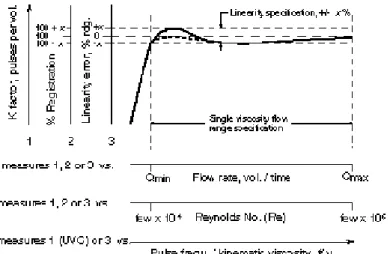
Fig. 12: typically shaped calibration curve of linearity versus flow rate for axial turbine meter (Wadlow (1998))... 45
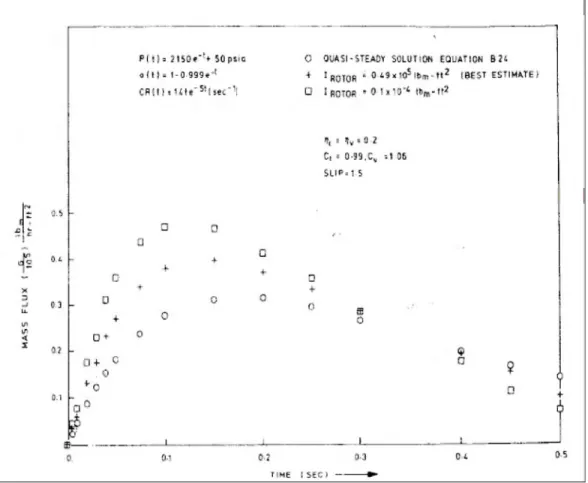
Fig. 13: Variation of the turbine meter response as a function of the rotor inertia (Hewitt (1978), based on Kamath and Lahey (1977) calculations)... 59
Fig. 14: Turbine meter velocities as a function of the air flow rate in two-phase vertical upflow, Hardy (1982)... 62
Fig. 15: Top Turbine flow meter (TFM) output predicted vs. observed values. (Shim (1997)) ... 65
Fig. 16: Drag disk scheme ... 66
Fig. 17: Typical Calibration Curve for Target flow Meters ... 68
Fig. 18: Full-flow drag disk... 69
Fig. 19: Drag coefficient of circular and square plates (in normal flow) as a function of Re (Averill and Goodrich) ... 70
Fig. 20: Drag disk frequency response... 77
Fig. 21: Drag disk and string probe data vs. measured mass flux for single and two phase flow (Hardy (1982)) ... 80
Fig. 22: Comparison of calculated with actual mass flux for single and two phase flow (Hardy (1982))... 81
Fig. 23: Comparison of differential pressure and drag body measurements across the tie plate, (Hardy and Smith (1990)) ... 82
Fig. 24: Comparison of momentum flux measured by the drag body with momentum flux calculated from measured data, Hardy and Smith (1990) ... 83
Fig. 25: Comparison of mass flow rate from measured inputs with a mass flow model combining drag body and turbine meter measurement, Hardy and Smith (1990) ... 84
Fig. 26: Flow through an orifice (top) and a Venturi tube (bottom) with the positions for measuring the static pressure (Jitshin (2004)) ... 85
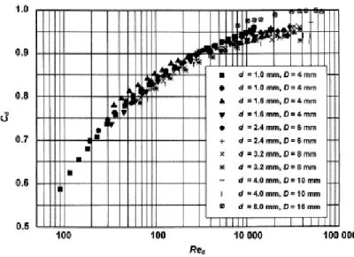
Fig. 27: Discharge coefficient of classical Venturi tubes with given throat diameters vs. Reynolds number. (Jitschin (2004)) ... 89
Fig. 28: Discharge coefficient of 6 Venturi tubes operated in normal direction (upper curves) and reversed direction (lower curves). (Jitschin (2004)) ... 89
Fig. 29: Orifice Flowmeter ... 94
Fig. 31: Vena-contracta for orifice meter (Omega Handbook (1995)) ... 95
Fig. 32: Venturi tube ... 97
Fig. 33: Venturi flowmeter types... 99
Fig. 34:Fluctuation of the DP signal of Venturi meter for single-phase flow obtained on the experimental setup (measured by a Si-element transmitter; the sample rate is 260 Hz). (a) Liquid flowrate is 13.04 m3/h, static pressure is 0.189 MPa and the temperature is 48.9 °C. (b) Gas flowrate is 98.7 m3/h, static pressure is 0.172 MPa and the temperature is 24.6 °C. (Xu et all (2003))... 100
Fig. 35: Nozzle flowmeter... 101
Fig. 36: Segmental Wedge element flowmeter ... 103
Fig. 37: V-cone flowmeter ... 104
Fig. 38: Pitot tube... 105
Fig. 39: Averaging Pitot Tube ... 107
Fig. 40: Elbow type flowmeter (efunda.com (2010)) ... 108
Fig. 41: Permanent pressure drop in differential flowmeter (EngineerinToolBox.com (2010))... 108
Fig. 42: Experimental pressure loss data for orifice tests (from Grattan et al. (1981) (Baker (1991)). ... 113
Fig. 43: Performance of orifice meter in an oil-water emulsion (from Pal and Rhodes (1985) ) (Baker (1991)) ... 113
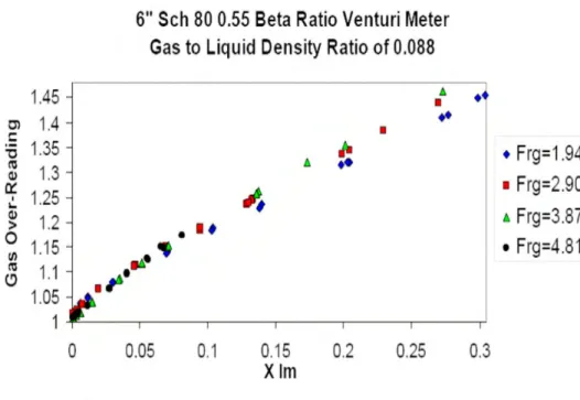
Fig. 44: X effect on the performance of a Venturi in two phase flow (Steven (2006)) ... 115
Fig. 45: Fr number effect on the performance of a Venturi in two phase flow (Steven (2006))... 116
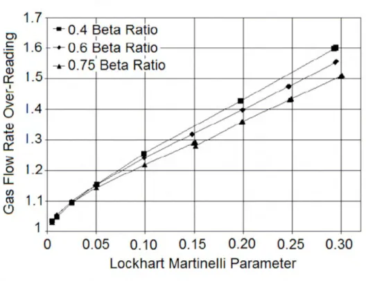
Fig. 46: Over reading of a Venturi meter measuring a wet gas flow at 15 bar and Fr = 1.5, for different β (Steven (2006) ... 117
Fig. 47: Comparison between the Venturi meter response obtained by NEL and by CEESI (Steven (2006))... 118
Fig. 48: Orifice meter over read as predicted by Murdock’s correlation, Kegel (2003). ... 120
Fig. 49: The original Murdock Two-Phase Flow Orifice Plate Meter Data Plot (Stenven (2006)) 121 Fig. 50: Venturi performance using Murdock correlation (Fincke (1999)) ... 123
Fig. 51: Gas mass flow rate error using Murdock correlation (Fincke (1999)) ... 124
Fig. 52: Measurement system scheme and Experimental procedure flow map (Oliveira et al. (2009)). ... 130
Fig. 53: Comparison between experimental and predicted quality using homogeneous and Zhang model... 131
Fig. 54: Comparison between experimental two phase flow rate and that predicted from correlations (Oliveira et al. (2009))... 132
Fig. 55 : Comparison of correlations at 20 bar, Steven (2002), ... 134
Fig. 56 : Comparison of correlations at 40 bar, Steven (2002). ... 135
Fig. 57 :Comparison of correlations at 60 bar, Steven (2002). ... 135
Fig. 58 Pressure drop in the Venturi, horizontal flow (Oliveira et al. (2009))... 138
Fig. 59: Pressure drop in the orifice plate, horizontal flow (Oliveira et al. (2009)) ... 138
Fig. 60: Relationship between ∆ and x (Xu et al. (2003)) ... 141 p Fig. 61: Relationship between I and x at 0.5 MPa ( Xu et al. (2003)) ... 141
Fig. 62: Relationship between I’ and x at all pressures (from 0.3 to 0.8 MPa) ( Xu et al. (2003)) 142 Fig. 63: Scheme of ring and concave type sensor ... 143
Fig. 69: Effect of the electrode spacing on the sensitivity of the ring type sensor... 158
Fig. 70: Effect of the electrode separation on the sensitivity for concave type sensor... 158
Fig. 71: Effect of the sensor dimensions on the sensitivity for concave type sensor ... 159
Fig. 72: Measured and theoretical dimensionless conductance for two different electrode spacing, ring electrodes under stratified flow conditions, Fossa (1998) ... 160
Fig. 73: Measured and theoretical dimensionless conductance for two different electrode spacing, ring electrodes under bubbly flow conditions. De indicates the distance between the electrodes, Fossa (1998) ... 161
Fig. 74: Measured and theoretical dimensionless conductance for two probe geometries: (a) ring electrodes D=70 mm, (b) ring electrodes D=14 mm. De indicates the distance between the electrodes, annular flow, Fossa (1998). ... 162
Fig. 75: Void fraction conductivity probe arrangement (G. COSTIGAN and P. B. WHALLEY (1996))... 169
Fig. 76: SCTF downcomer probe ... 170
Fig. 77: Drag disk and string probe data vs actual the mass flow rates for both single phase and two-phase flow (Hardy (1982)) ... 171
Fig. 78 : Comparison between the mass flux calculated with the calibration correlations and the actual mass flux for both single and two-phase flow (Hardy (1982)) ... 172
Fig. 79: Comparison of liquid fraction from string probe and three beam gamma densitometer (Hardy (1982)) ... 173
Fig. 80: Actual mass flow rate compared with the mass flow rate calculated with the homogeneous model (Hardy (1982)) ... 174
Fig. 81: String probe used by Hardy et all. (1983) ... 175
Fig. 82: Void fraction comparison for string probe and three beams gamma densitometer (both level of sensor presented), Hardy and Hylton (1983) ... 176
Fig. 83: Velocity comparison of the string probe and turbine meter (Hardy and Hylton (1983)) .. 178
Fig. 84: (left) Principle of wire-mesh sensor having 2 x 8 electrodes. (right) Wire-mesh sensor for the investigation of pipe flows and associated electronics... 180
Fig. 85: 3D-Visualization of data acquired with a wire-mesh sensor in a vertical test section of air-water flow at the TOPFLOW test facility. ... 181
Fig. 86: EIT electrode configuration... 186
Fig. 87: Block diagram of ECT or ERT system ... 187
Fig. 88: Measuring principles of ECT (left) and ERT (right) ... 188
Fig. 89: ERT for water-gas flow (Cui and Wang (2009))... 188
Fig. 90: Flow Pattern recognition (Wu and Wang) ... 191
Fig. 91: Cross-correlation between two image obtained with dual-plane ERT sensor (Wu and Wang) ... 191
Fig. 92: Correlation local velocity distribution and mean cross-section gas concentration at different flow pattern. (Wu and Wang) ... 192
Fig. 93: EIT strip electrode array. The bottom scale is in inch (George et all (1998) ... 196
Fig. 94: Flow chart of EIT reconstruction algorithm (George et all. (1998)) ... 197
Fig. 95: Comparaison of symmetric radial gas volume fraction profile from GDT and EIT (George et all. (1999)) ... 198
Fig. 96: Comparisons of reconstruction results using NN-MOIRT and other techniques (Warsito and Fan (2001))... 200
Fig. 97: Comparisons of time average sectional mean gas holdup and time-variant cross-sectional mean holdup in gas–liquid system (liquid phase: Norpar 15, gas velocity=1 cm/s). (Warsito and Fan (2001)) ... 201
Fig. 98: Design of flow pattern classifier and Void fraction measurement model (Li et all (2008) 203 Fig. 99: Voidage measurement process (Li et all (2008) ... 204
Fig. 101: ECT sensor mounted on transparent plastic pipe with electrical guard removed for clarity.
(Azzopardi et all. (2010)) ... 205
Fig. 102: 24×24 wire-mesh sensor for pipe flow measurement. (Azzopardi et all. (2010)) ... 206
Fig. 103: Comparison of overall averaged void fraction from Wire Mesh Sensor and Electrical Capacitance Tomography (first campaign). (Azzopardi et all. (2010))... 206
Fig. 104: Comparison of overall averaged void fraction from Wire Mesh Sensor and Electrical Capacitance Tomography (second campaign). (Azzopardi et all. (2010)) ... 207
Fig. 105: Comparison between WMS (both conductance and capacitance) and gamma densitometry. Gamma beam placed just under individual wire of sensor. (Azzopardi et all. (2010)) ... 207
Fig. 106: Mean void fraction – liquid superficial velocity =0.25 m/s - closed symbols – water; open symbols = silicone oil. (Azzopardi et all. (2010)) ... 208
Fig. 107: Electric probe signals displaying different flow regimes... 211
Fig. 108: Illustration of PD determination (Rouhani et Sohal (1982)) ... 215
Fig. 109: PDF of bubbly flow (Jones and Zuber (1975))... 218
Fig. 110: PDF of slug flow (Jones and Zuber (1975)). ... 218
Fig. 111: PDF of annular flow (Jones and Zuber (1975)). ... 219
Fig. 112: PDF of bubbly flow. A photograph (a), diameter PDF (b), and diameter PSD (c) for 13% area-averaged void fraction, jl = 0.37 m/s, jg= 0.97 m/s (Vince and Lahey (1980)) ... 220
Fig. 113: PDF variance and indication of regime transition (Vince and Lahey (1980)) ... 221
Fig. 114: Cumulative PDF from different sensors analysis (Keska (1998)) ... 224
Fig. 115: Comparison of RMS values of each signal obtained from four methods at different flow pattern (Keska (1998)) ... 225
List of Tables:
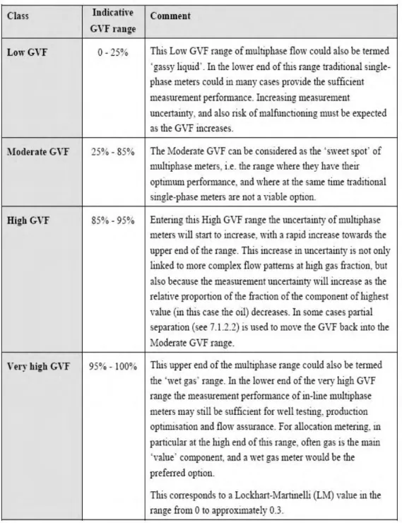
Tab. 1: Some of flow pattern map coordinates... 13Tab. 2: Classification of Multiphase flow, based on void fraction value (HMPF (2005)) ... 15
Tab. 3: Selection of sensor (Yeung and Ibrahim, 2003) ... 25
Tab. 4: Differential pressure meter comparison ... 90
Tab. 5: Parameters used in the flowrate measurement correlations for different flow patterns (Meng (2010))... 125
Tab. 6: Comparison results of flowrate measurement correlations for different flow patterns (Meng (2010))... 126
Tab. 7: Root mean square fractional deviation for the whole data set (all pressures) and for each individual pressure, Steven (2002). ... 134
Tab. 8: k and b values ( Xu et al. (2003))... 142
Tab. 9: void fraction measured with different techniques... 146
Tab. 10: Material tested for thermal shocks (Moorhead and Morgan (1978) ... 167
1. Introduction
The measurement of two-phase flow quantities is essential for the understanding of many technical processes, especially reactor system behaviour under accident conditions, and is also a prerequisite for proper code modelling and verification. More than 25 years have been spent on developing various solutions for measuring two-phase flow with the aim to:
- obtain local or integral information,
- build very sensitive (but usually also fragile) instruments and try to improve the precision of the more rigid sensors as well, and
- apply techniques that are simple to use and to interpret and to install highly sophisticated instruments.
In spite of these efforts, there is no and perhaps never will be a Standard or Optimum Instrumentation. Measuring two-phase flow will always require experienced researchers using special solutions for each required purpose.
Successful application of a measuring system in a two-phase test setup does not automatically guarantee its applicability for nuclear reactor conditions, or even for other test loops if environmental conditions such as radiation levels or even simply water quality change. In addition, two-phase measuring techniques in many cases do not measure directly the two-phase properties
(such as local shear, velocities of the single phases etc.) needed to verify the two-phase models so that indirect comparison of calculated and measured data is needed.
Despite these not very encouraging facts, the large reactor safety research programs performed in the last decade as well as the detailed development work carried out at numerous universities and research institutions have significantly increased our knowledge of two-phase flow measurement techniques.
But the key to fundamental understanding of two-phase flow is still careful development of specialized instrumentation, in particular for special and complex geometrical applications.
In addition, development of special algorithms is sometimes necessary to interpret the measurement signals under many possible two-phase conditions.
2. TWO PHASE FLOW PARAMETERS
Multiphase flow is a complex phenomenon which is difficult to understand, predict and model. Common single-phase characteristics such as velocity profile, turbulence and boundary layer, are thus inappropriate for describing the nature of such flows.
The flow structures are classified in flow regimes, whose precise characteristics depend on a number of parameters. The distribution of the fluid phases in space and time differs for the various flow regimes, and is usually not under the control of the designer or operator.
Flow regimes vary depending on operating conditions, fluid properties, flow rates and the orientation and geometry of the pipe through which the fluids flow. The transition between different flow regimes may be a gradual process.
The parameters used to characterise the two phase flow are: − Mass flow and velocity
− Temperature − Void fraction − Local void fraction − Critical heat flux
− Liquid level and film thickness − Flow regimes
− Wall shear stress and turbulence − Velocity distribution
The determination of flow regimes in pipes in operation is not easy. Analysis of fluctuations of local pressure and/or density by means of for example gamma-ray densitometry has been used in experiments and is described in the literature. In the laboratory, the flow regime may be studied by direct visual observation using a
The main mechanisms involved in forming the different flow regimes are transient effects, geometry effects, hydrodynamic effects and combinations of these effects.
For a complete review on flow pattern see Rouhani et Sohal (1982).
Transients occur as a result of changes in system boundary conditions. This is not to be confused with the local unsteadiness associated with intermittent flow. Opening and closing of valves are examples of operations that cause transient conditions.
Geometry effects occur as a result of changes in pipeline geometry or inclination. In the absence of transient and geometry effects, the steady state flow regime is entirely determined by flow rates, fluid properties, pipe diameter and inclination. Such flow regimes are seen in horizontal straight pipes and are referred to as “hydrodynamic” flow regimes.
All flow regimes however, can be grouped into dispersed flow, separated flow, intermittent flow or a combination of these (see Fig. 1 and Fig. 2)
• Dispersed flow is characterised by a uniform phase distribution in both the radial and axial directions. Examples of such flows are bubble flow and mist flow. • Separated flow is characterised by a non-continuous phase distribution in the radial direction and a continuous phase distribution in the axial direction. Examples of such flows are stratified and annular .
• Intermittent flow is characterised by being non-continuous in the axial direction, and therefore exhibits locally unsteady behaviour. Examples of such flows are elongated bubble, churn and slug flow. The flow regimes are all hydrodynamic two-phase gas-liquid flow regimes.
Fig. 1: Schematics of horizontal flow regimes
Fig. 2: Schematics of vertical flow regimes
For a quantitative description of the conditions which lead to the transition of flow regimes from one pattern to another it is necessary to define a set of parameters or parameter groups which show a direct bearing on such transitions. In a simplistic approach two of the main flow parameters may be used to define a coordinate system in which the boundaries between different flow regimes may be charted.
perhaps adequate for identifying the operating conditions that specify various regimes for a given fluid in a fixed geometry (pipe diameter and wall surface nature). But it would not be useful for making any generalization to other fluids or other geometries regarding the conditions which would cause flow regime transitions. This is because many different parameters affect the occurrence of various flow regimes and it is not possible to represent flow regime transition criteria in terms of only two simple variables.
Baker (1954) was one of the first ones to use some relevant groups of flow variables as flow regime
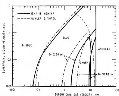
description coordinates. Baker's flow regime map was based on observations on cocurrent flow of gaseous and condensate petroleum products in horizontal pipes The diagrams in Fig. 3 is qualitative illustrations of how flow regime transitions are dependent on superficial gas and liquid velocities in vertical multiphase flow. In Fig. 4 is illustrate the Taitel and Dukler’ map for horizontal flow, and in Fig. 5 a comparison is made for vertical flow, with Ishii and Mishima’s map.
Although Baker's flow map coordinates includes these apparently relevant variables for scaling a variety of different conditions, later investigations showed that this map did not adequately predict horizontal flow regimes in all situations. There are many other coordinate systems for flow regime maps suggested by different investigators. A few of these are summarized in Tab. 1.
Fig. 5: Comparison of the verical flow pattern maps of Ishii and Mishima (1980) with of Taitel and Dukler.
Another way to classify multiphase flow, apart from the classification according to the flow pattern, is by the void fraction value of the flow. This method of classification is relevant to multiphase metering; a meter measuring predominately liquid with just a few percent gas would be significantly different from one designed to operate in what is generally understood as a wet gas application. Four classes are defined in Tab. 2
3. INSTRUMENTS CLASSIFICATIONS
The needs of the chemical, petrochemical, gas and oil pipeline, and nuclear industries and the availability of advanced signal-processing techniques stimulate rapid developments in instrumentation applicable to two-phase flow measurements.
The objective of multiphase flow metering is to determine the flow rates of the individual components, for example water and gas or water and steam.
Unfortunately there is no single instrument, which will measure these parameters directly and it is necessary to combine several devices in an instrument package and to calculate the specific flow rates from the combined readings. There are many possible combinations, and the number of instruments required depends upon whether or not the components can be mixed together upstream of the instrumentation (homogeneous flow). If homogeneity of flow can be achieved, then only three instruments are required, each measuring a characteristic of the mixed fluid flow; if not, then individual component velocities and concentrations have to be determined.
Excellent reviews have been written on the state of the art of two-phase flow instrumentation. See, for example, Baker (2000), Hewitt (1978), and Miller (1996).
In the previously paragraph the parameters that characterized the two phase flow has been defined.
For measurement purpose an instrument classification can be made considering which parameter can be measured and through which physical principle the instrument operate.
The following main categories can be applied: • In-line meters
• Separation type meters
− Full two-phase gas/liquid separation − Partial separation
− Separation in sample line
In-line meter performed directly in the multiphase flow line, hence, no separation and/or sampling of the fluids are required.
The volume flow rate of each phase is represented by the area fraction multiplied by the velocity of each phase. This means that a minimum of six parameters has to be measured or estimated (T, p, v, W, x, alpha or ρ).
Meter classification considering the parameter measured is: − Density( ρ ) meter
− Velocity (v ) meter − Momentum (ρv2) meter − Mass flow (ρv) meter
The physical principles of the different flow meter are: − Mechanical
− Hydraulic − Acoustic − Electrical
− Gamma and X-ray − Neutrons
− Microwave attenuation − Infrared spectroscopy
The different physical working principle are used to measure different parameters (Baker (2000)):
Measurement of density (ρ) − Gamma-ray (γ) absorption − Neutron (n) interrogation − Weighing of tube
− Hot film anemometer
− Capacitance / Conductance probes − Ultrasonic flowmeter
Measurement of velocity (v) − Pulsed-neutron activation − Electromagnetic flow meter
− Capacitance/conductivity cross correlation − Laser Doppler velocimeter
Measurements of mass flow (ρv) − True mass flow meter − Vibrating tube
− Differential pressure flowmeters Measurements of momentum flux (ρv2)
− Venturi meter − Drag Disk
The choice of a meter (involving at least two separate measuring devices) to measure flow rates in two-phase flow (Hewitt 1978) depends on the purpose for which the measurement is made, and the accuracy required. It also depends on the nature of the flow field and the two phases involved.
The devices employed can be either nonintrusive (external to the flow field or, at most, part of the pipe/fluid interface) or intrusive (thus distorting the flow geometry at the place of measurement).
Nonintrusive devices can use tomographic techniques to sense local characteristics of the motion. Some intrusive devices provide global measurements, and some (local optical, electrical, or pressure probes) provide local phase flow rates.
The relative magnitudes of the instrumental length scales (pipe diameter, probe tip radius, piezoelectric crystal diameter), the dispersed phase length scale (particle, drop or bubble “diameters,” film thickness), and the wave length of the sensing radiation (whether electromagnetic or acoustic) restrict the nature of the information provided by any device and hence affect how fluxes are deduced. It is almost always helpful to have overall kinematic information about phase distributions and phase velocities when selecting a measurement technique for a particular flow.
The measurement of two-phase mass flow rate is of primary importance in experimental programs involving loss-of-coolant studies. Because of the severe environments present during blowdown, relatively few instrument types have gained widespread acceptance; these include turbine meters, gamma densitometers, and drag flowmeters. (Pressure and temperature measurements are
also required for reduction of data from the other instruments.) located in a relatively short piping segment called a spool piece. The design of spool pieces is important because intrusive meter may seriously alter the flow regime. On the other hand, location of all the instruments in close proximity is desirable because of the often unsteady and inhomogeneous nature of two phase flow.
In the last few years many efforts were made by scientists all over the world to understand the physics of the chain ‘pipe configuration-disturbed flow profile-change in flowmeter behaviour and to find out effective methods and techniques to minimise these installation effects.
The relation between disturbed flow profile and change of flowmeter behaviour alone already presents a huge field of problems. Installation effects basically depend on the technical principle and construction of the flowmeter itself. The resulting problems are therefore unique for every type of flowmeter.
One truly two-phase fluid is steam. Superheated steam may be treated as a gas and its properties are well tabulated. However, it is increasingly important to measure the flow of wet steam made up, say, of about 95 per cent (by mass) vapour and about 5 per cent liquid. The droplets of the liquid are carried by the vapour, but will not follow the vapour stream precisely.
The measurement of such a flow causes major problems, since the pressure and temperature remain constant while the dryness fraction changes. It is therefore not possible to deduce the dryness fraction or density from the pressure and temperature, and in addition the droplets will cause an error in the flowmeter’s registration.
These complex flows have been extensively studied, and flow pattern maps have been developed to indicate the conditions under which the various flow regimes occur.
However, these tend to be limited in their application to particular fluid combinations and pipe sizes.
The response of a meter in two-phase flow tends to be high sensitive to the flow pattern and to the upstream configuration and flow history. The best practice is to
Though the ideal is to use in situ calibration, the more usual method is to interpret the measurement from an instrument in terms of a theory whose validity is tested by conducting separate experiments. Very often these experiments are conducted for very different flow conditions and fluids: instruments used for steam/water flows are frequently calibrated using air/water flows.
The response of a flowmeter may be different in transient situation and it’s better to find a way to correct for this.
The basis of proper meter selection is a general awareness of flow measurement science and a clear understanding of specific application requirements.
General Meter Selection Factors
For end users, there are a number of specific issues to keep in mind when choosing a flow-metering instrument. Different flowmeters are designed for optimum performance in different fluids and under different operating conditions. That’s why it is important to understand the limitations inherent to each style of instrument. Measuring the flow of liquid and gases (two- phase flow) demands superior instrument performance. In the reactor studies context this measurement is complicated by the fact that during the transient, the fluid becomes a nonhomogeneous mixture of liquid water and steam at. or very near saturation. In addition, materials from which the transducer is fabricated must be carefully chosen for their ability to survive the destructive effects of the water chemistry and radiation.
Process Conditions
In high-pressure flow applications, the “water hammer” effect can severely damage conventional flow measurement devices. Water hammer (or, more generally, fluid hammer) is a pressure surge or wave caused by the kinetic energy of a fluid in motion when it is forced to immediately stop or change direction. For example, if a valve is closed suddenly at an end of a pipeline system, a water hammer wave propagates in the pipe. Ideally, an industrial flowmeter, whether it employs mechanical or electromagnetic principles, should respond instantly and consistently to changes in water velocity. Meters, however, are not perfect instruments and may not accurately register velocity in all measurement conditions encountered. Turbulent or pulsating flows can cause registration errors in meters. In recent years, instrument suppliers have developed new PD meter
configurations for pulsating flow streams encountered in batch applications. These meters, employing a bearingless design and non-intrusive sensors.
Flowmeter Accuracy
In situations where flowmeters are used to give an indication of the rate at which a liquid or gas is moving through a pipeline, high accuracy is not crucial. But for batching, sampling and dispensing applications, flowmeter accuracy can be the deciding factor between optimum quality and wasted product. Typically, flowmeter accuracy is specified in percentage of actual reading (AR), in percentage of calibrated span (CS), or in percentage of full-scale (FS) units. Accuracy requirements are normally stated at minimum, normal, and maximum flow rates. The flowmeter’s performance may not be acceptable over its full range.
Response time is another key flowmeter performance criteria.
Fluid Compatibility
For special applications flowmeters can be constructed with specialized materials. In addition to 316 stainless steel and Hastelloy, standard flowmeter wetted parts are manufactured from Tantalum, Monel, Nickel, Titanium, Carbon Steel, and Zirconium. Flowmeter manufacturers have invested considerable time and resources to develop meter designs utilizing thermoplastic materials able to handle corrosive liquids and gases. For example, all-plastic PD meters are ideal for aggressive liquid flow applications, including acids, caustics, specialty chemicals, and DI water. Ultrasonic flowmeters have no moving or wetted parts, suffer no pressure loss, and provide maintenance-free operation— important advantages over conventional mechanical meters such as vortex meters, and also, in many cases, coriolis mass meters. Clamp-on ultrasonic meters are mounted completely external to the pipe wall, so they are not affected by corrosive or erosive liquids, and are not damaged by solids, gases or particles in the process liquid.
of available installation space may dictate the choice of flowmeter technology. Where there is limited room, larger instrument designs like Coriolis meters may not be feasible. Vortex, turbine and PD meters, as well as a handful of other technologies, are a wiser choice under these circumstances. Nearly all flow instruments must be installed with a significant run of straight pipe before and after the location of the meter. Elbows, reducers, chemical injection ports, filters, screens and valves can cause radial, tangential and axial swirling effects within the pipe. In combination, these changes can rapidly distort the velocity profile, degrading the flowmeter’s accuracy and repeatability. Many flow measurement instruments require straightening vanes or straight upstream piping to eliminate distorted patterns and swirls. This involves the installation of additional diameters of straight pipe run before the flow straightener, and between the straightener and the flowmeter itself.
Maintenance Needs
Flowmeters with few or no moving parts require less attention than more complex instruments. Meters incorporating multiple moving parts can malfunction due to dirt, grit and grime present in the process fluid. Meters with impulse lines can also plug or corrode, and units with flow dividers and pipe bends can suffer from abrasive media wear and blockages. Moving parts are a potential source of problems, not only for the obvious reasons of wear, lubrication and sensitivity to coating, but also because they require clearance spaces which sometimes introduce “slippage” into the flow being measured. Even with well-maintained and calibrated meters, this unmeasured flow varies with changes in fluid viscosity and temperature. Temperature changes also change the meters internal dimensions and require compensation.
Flow-meter selection criteria for the SPES 3 facility
The most important criteria that the flow-meter has to satisfy, are listed below, with a brief explanation:
Two phase flow handling capability and easy modelling
Existing experimental evidence the meter design can effectively handle two-phase flow is a required prerequisite, since new meter concepts cannot be explored in industrial testing. First approximated modelling capability of the meter response is as well required. Two-phase flow metering is not standardized, so that meters response has to be somewhat tailored for every application. In this respect, a highly sophisticated instrument that is to be taken as a black box is not suited for practical use.
High Span (minimal number of parallel lines)
The break flow is expected to vary in a wide range, so that the capability of the meter to cover a huge span is a good prerequisite. If a wide range meter is not available, the only solution is to build a proper number of parallel lines in order to use more than one meter for different mass flow rates.
Good Repeatability and Accuracy
The repeatability of the instruments has to be as good as possible in order to guarantee the correspondence of values collected in different times, but in the same operation condition.
Minimal Installation Constraints (straight pipe length between the meter and the disturbance source) -A minimal straight pipe length is required in front and after the instrument in order to avoid disturbance to the velocity profile.
A distorted profile (different from the complete developed profile) could cause an error in the instrument response.
Simplicity of Calibration; effects of calibration and operation temperature differences (different fluid properties, flow-meter material expansion)
The meter has to be as independent as possible from the temperature difference between the calibration and the operation condition. Calibration in cold conditions is easier, while specific facilities are required in hot conditions and the costs
Capability of Handling Different Flow Regimes (temperature range, pressure range)
There are some cases in which the flow is far away from being homogeneous, because particular temperature and pressure conditions could cause the separation of the two phases. These different types of flow regime could cause a misleading response of the flow-meter, because not all the flow-meters are able to spanning all the pipe section to detect average values of the measured quantity.
Transient Operation Capability (time response)
Since the break discharged flow is not steady state, a good transient capability is a required prerequisite. The capability to follow fast transient is required, or at least the capability to mathematically model the dynamic response of the meter so as to correct the signal for dynamic effects.
Bi-directional Operation Capability
Both Reactor Pressure Vessel discharge into the Containment and possible reverse flow from the Containment into the Reactor Pressure Vessel have to be measured. Minimal Regulatory Requirements
The process that leads to the installation of the instruments has to be as fast as possible, according with the current legislation.
Suitable Physical Dimension
Instrumentation dimensions and weight need to be consistent with the available space and support facilities. The instruments dimensions are likely to be the more critical issue.
Minimal Disturbance to the Flow
In order to avoid any significant alteration of the thermal-hydraulic coupling between the Reactor Pressure Vessel and the Containment that could drive somewhat the testing and that the testing is intended to explore, the disturbance to the discharged flow caused by the meter should be as low as possible.
Simplicity of Data Acquisition
The instrumentation needed to collect the data generated by the flow-meter has to operate independently from the fluid conditions and the necessary power supply and electrical equipment has to cope with the SIET available facilities.
Capability of Operating in Different Assembling Orientation (horizontal, vertical, inclined)- Some meters require particular assembling orientation in order to avoid inhomogeneous configuration of the flow pattern and entrapment of
gas bubbles near to the sensors position, both leading to an incorrect measurement of the fluid flow. This constraint could be an issue for the design of the SPES3 pipelines, because of the spatial orientation of the pipes.
Cavitation
The cavitation phenomenon should be avoided.
In the 2003 Yeung and Ibrahim proposed a selection of multiphase sensors based on the following criteria:
1. known behaviour in oil/water/gas flows 2. frequency (or dynamic response) 3. complexity of sensor output processing 4. commercial availability
5. cost
6. non-intrusive design 7. reproducibility
8. ruggedness/complexity
Based on the analysis of previous works they built the following table:
This searches could miss relevant papers and many papers are necessarily covered only very briefly.
It is not possible to cover the subject exhaustively here, so we restrict the analysis at only few instruments. The reader is referred to the books by Baker (2000) for more information.
4. TURBINE METERS
The turbine-meter is essentially a turbine rotor which rotates as the fluid passes through its blades. The turbine output, registering a pulse for each passing blade, can be used to calculate the fluid velocity and the Volumetric flux; is actually the most important volumetric meter.
According to the installed direction of a rotor shaft, two types of turbine flowmeter are available: axial type turbine flowmeter and tangential type turbine flowmeter, and the axial type turbine flowmeter is usually called a turbine flowmeter now.
The original tangential type turbine flowmeter (Stine (1977)) was invented in 1961 and is used to measure micro-flow rate. This type of the meter does not have wide application because of its unformed structure. However, some performances of a tangential type turbine flowmeter are still better than a turbine flowmeter, such as lower limit of measurement range, higher sensitivity and faster dynamic response. In general, the research on tangential type flowmeters is still limited now.
The modern axial turbine flowmeter, when properly installed and calibrated, is a reliable device capable of providing high accuracies (of about 0.2%) for both liquid and gas volumetric flow measurement.
General performance characteristics
Axial turbines perform best when measuring clean, conditioned, steady flows of gases and liquids with low kinematic viscosities (below about 10-5 m2s-1, 10 cSt, although they are used up to 10-4 m2s-1, 100 cSt), and are linear for subsonic, turbulent flows. Under these conditions the inherent mechanical stability of the meter design gives rise to excellent repeatability performance.
The main performance characteristics are:
• Sizes, (internal diameter) range from 6 to 760 mm , (1/4'' - 30'').
• Maximum measurement capacities range from 0.025 Am3/hr to 25,500 Am3/hr, (0.015 ACFM to 15,000 ACFM), for gases and 0.036 m3/hr to 13,000 m3/hr, (0.16 gpm to 57,000 gpm or 82,000 barrels per hour), for liquids, where A denotes actual.
• Typical measurement repeatability is 0.1% of reading for liquids and 0.25% for gases with up to 0.02% for high accuracy meters. Typical linearities, (before electronic linearization), are between 0.25% to 0.5% of reading for liquids and 0.5% and 1.0% for gases. High accuracy meters have linearities of 0.15% for liquids and 0.25% for gases, usually specified over a 10:1 dynamic range below maximum rated flow.
• Rangeability, when defined as the ratio of flow rates over which the linearity specification applies, is typically between 10:1 and 100:1.
• Operating temperature ranges span -270oC to 650oC, (-450oF to 1200oF).
• Operating pressure ranges span coarse vacuum to 414 MPa, (60,000 psi).
• Pressure drop at the maximum rated flow rate ranges from around 0.3 kPa (0.05 psi) for gases to in the region of 70 kPa (10 psi) for liquids.
Theory
Tangential type
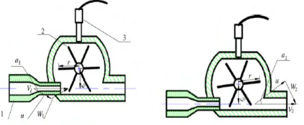
The principal configuration of the tangential type turbine flowmeter is shown in Fig. 1. Annotation 1 is the jet, 2 is the rotor-blade, and 3 is the magnetic pickup. When fluid flow through the rotor-blade is in the tangential direction, fluid drives the rotor-blade to rotate anti-clockwise. In order to improve the driving force, the jet is installed at the inlet of the meter, and the measurement range can be changed by altering the diameter of the jet outlet aperture. The rotational speed of the rotor-blade can be obtained by the magnetic pickup.
Fig. 7: a. Inlet velocity triangle of tangential type turbine flowmeter, b.Outlet velocity triangle of tangential type turbine flowmeter.
The velocity vector triangle of a tangential type turbine flowmeter at inlet and outlet is shown in Fig. 7, where W1 is inlet relative velocity, W2 is outlet relative velocity which is tangential with the outlet rotor blade, U1 and U2 are circular velocity, and r0 is the distance between the shaft and the axis of jet outlet.
The equation of the meter performance is developed from a torque balance on the rotor-blade as below (Zheng and Tao (2007)):
0 r rm rf re
rotor’s rotational speed, Trf becomes bigger. When the rotor is in the steady
operation situation, Trm << Trf is taken. So Trf plays an important position while
Trm is neglected.
Usually Tre is very small and can be regarded as zero, so Tre is neglected. Under
steady flowing condition, the rotor is in the balance of rotating. The main factor affecting meter performance is Trf, so a new equation for the meter performance is developed from a torque balance on the rotor as below:
0 r rf
T −T =
When the fluid is flowing through the meter, usually, under the turbulence flow condition, Trf is represented as follows:
2
rf
T =C Qρ where C is constant.
According to the momentum equation, the rotor driving torque Tris represented as
follows:
(
1 cos 1 2 cos 2)
r
T =ρQ V r α −V r α
where ρ is fluid density, Q is volumetric flow rate, r is radius of rotor, α1 is the
angle between V1 and U1, and α2 is the angle betweenV2 and U2.
The fluid absolute velocity V1 at jet outlet is presented as follows:
1 Q V
A
=
where A is the area of jet outlet aperture.
According to the outlet velocity triangle, the following equation can be presented 2 cos 2 2 0
V r α = =u πr n
where n is rotor rotary speed.
According to Fig. 7, r0 is presented as:
0 cos 1 r =r α
Substituting into the first equation to obtain the rotor driving torque Tr :
2 0 2 r Q T Q r r n A ρ π = −
The tangential type turbine flowmeter performance is described by a volumetric meter factor K as follows:
f K
Q
=
where f is pulse frequency,
f =Z n⋅
where Z is the number of rotor blades.
Combining the equations, the tangential type turbine flow meter performance equation is given as:
0 2 2 r Z K C r A π = −
The following conclusions can be obtained from the above equation: meter factor
K is only affected by the meter structural parameter, while it is not affected by volumetric flow rate, density, etc. So K can be regarded as a constant value (Zheng and Tao (2007)).
Axial type
There are two approaches described in the current literature for analyzing axial turbine performance.
The first approach describes the fluid driving torque in terms of momentum exchange, while the second describes it in terms of aerodynamic lift via airfoil theory (Thompson (1970)). The former approach has the advantage that it readily produces analytical results describing basic operation, some of which have not appeared via airfoil analysis.
The latter approach has the advantage that it allows more complete descriptions using fewer approximations. However, it is mathematically intensive and leads rapidly into computer generated solutions. One prominent pioneer of the momentum approach is Lee (1965) who, using this approach, later went on to invent one of the few, currently successful, dual rotor turbine flowmeters, while Thompson and Grey (1970) provided one of the most comprehensive models
In a hypothetical situation, where there are no forces acting to slow down the rotor, it will rotate at a speed which exactly maintains the fluid flow velocity vector at the blade surfaces.
Fig. 8: Vector diagram for a flat-bladed axial turbine rotor. The difference between the ideal (subscript i) and actual tangential velocity vectors is the rotor slip velocity and is
caused by the net effect of the rotor retarding torques.
This gives rise to linearity errors and creates swirl in the exit flow. V incident fluid velocity vector; VE exit fluid velocity vector; θ exit flow swirl angle due to rotor retarding torques; β blade pitch angle, same as angle of attack for parallel flow; ω rotor angular velocity vector; r rotor radius vector; F flow induced drag force acting on each blade surface; c blade chord; s blade spacing along the hub; c/s rotor solidity factor.
Fig. 8 is a vector diagram for a flat bladed rotor with a blade pitch angle equal to β. Assuming that the rotor blades are flat and that the velocity is everywhere uniform and parallel to the rotor axis, then referring to Fig. 8:
tan i
rω =V β
When one introduces the total flow rate this becomes:
tan i
Q rA
ω β
=
Where ωiis the 'ideal' rotational speed, Q is the volumetric flow rate, A is the area
of the annular flow cross section and r is now the root-mean-square of the inner and outer blade radii, (R, a). Eliminating the time dimension from the left hand
side quantity reduces it to the number of rotor rotations per unit fluid volume, which is essentially the flowmeter K factor specified by most manufacturers. Hence, according to the second equation, in the ideal situation the meter response is perfectly linear and determined only by geometry. In some flowmeter designs the rotor blades are helically twisted to improve efficiency. This is especially true of blades with large radius ratios, (R/a). If the flow velocity profile is assumed to be flat, then the blade angle in this case may be described by tanβ =constant · r. This is sometimes called the 'ideal' helical blade. In practice, there are instead a number of rotor retarding torques of varying relative magnitudes. Under steady flow the rotor assumes a speed which satisfies the following equilibrium:
Fluid driving torque = rotor blade surfaces fluid drag torque + rotor hub and tip clearance fluid drag torque + rotation sensor drag torque + bearing friction retarding torque
Referring again to Fig. 8, the difference between the actual rotor speed, rω, and the ideal rotor speed, rωi, is the rotor slip velocity due to the combined effect of all the rotor retarding torques as described in the equilibrium equation above, and as a result of which the fluid velocity vector is deflected through an exit or swirl angle, θ. Denoting the radius variable by r, and equating the total rate of change of angular momentum of the fluid passing through the rotor to the retarding torque, one obtains:
which yields:
(
i)
NTQ
r2ρ ω −ω =
The trends evident in the obtained equation reflect the characteristic decline in meter response at very low flows and why lower friction bearings and lower drag pickups tend to be used in gas versus liquid applications and small diameter meters. In most flowmeter designs, especially for liquids, the latter three of the four retarding torques described in the equilibrium equation are small under normal operating conditions compared with the torque due to induced drag across the blade surfaces. As shown in Fig. 8, the force, F, due to this effect acts in a direction along the blade surface and has a magnitude given by:
where CD is the drag coefficient and S is the blade surface area per side. Using the
expression for drag coefficient corresponding to turbulent flow, selected by Pate et al. (1984) and others, this force may be estimate by:
20.074 Re 0.2 F =ρV − S
where Re is the flow Reynolds number based on the blade chord shown as dimension c in Fig. 8. Assuming θ is small compared with β, then after integration, the magnitude of the retarding torque due to the induced drag along the blade surfaces of a rotor with n blades is found to be:
(
R a)
ρV20.037Re 0.2Ssinβ n ND = + − Combining whit: 2 2 tan Q r N A r Q T ρ β ω − =and rearranging yields:
(
)
2 2 2 . 0 sin Re 036 . 0 tan r SA a R n A r Q β β ω − + − =That is an approximate expression for K factor because it neglects the effects of several of the rotor retarding torques, and a number of important detailed meter design and aerodynamic factors, such as rotor solidity and flow velocity profile. Nevertheless, it reveals that linearity variations under normal, specified operating conditions are a function of certain basic geometric factors and Reynolds number. These results reflect general trends which influence design and calibration. Additionally, the marked departure from an approximate ρV2 (actually
0.8 1.8 0.2 V ρ µ−
via Re) dependence of the fluid drag retarding torque on flow properties under turbulent flow, to other relationships under transitional and laminar flow, gives rise to major variations in the K factor versus flow rate and media properties for low flow Reynolds numbers. This is the key reason why axial turbine flowmeters are generally recommended for turbulent flow measurement.
Dynamic response of axial turbine flowmeter in single phase flow
Turbine flowmeters are essentially instruments for metering steady flows, but it is often argued that their responsiveness makes them suitable for metering flows in which a degree of unsteadiness is present.
The dynamic response of turbine flowmeters in low density (gas) flows is relatively well understood and methods are available for the correction of errors due to over-registration in pulsating flows. The work of Ovodov et al. (1989) on liquid nitrogen indicated problems of predicting transient behaviour without knowing the dynamic characteristics of the meter.
Some items of plant can cause approximately sinusoidal pulsations, such as reciprocating pumps or unstable control valves in a pipeline. The dynamic response of turbine flowmeters in low-pressure gas flows (where the rotational inertia of the fluid is negligible) is well understood and methods for correcting meter signals for a lack of response are available. Turbine flowmeters in liquid flows are expected to be subject to similar errors although the relevant ranges of pulsation frequency and amplitude are expected to be different.
where Va ⋅
is the mean volume flow rate and fp is the pulsation frequency. When the meter is subjected to Va
⋅
, the rotor responds and rotates with angular velocity ω(t), and the meter indicated volume flow rate, Vm
⋅
, can then be evaluated. It is of interest to investigate this time dependent response of the meter to the driving flow rate.
According to BS ISO TR 3313 (1998), when a turbine flowmeter is operating within a pulsation cycle, the inertia of the rotor (and possibly of the fluid contained within the rotor envelope) can cause the rotor speed to lag behind the steady state condition in an accelerating flow and to exceed it in a decelerating flow.
The response of a meter to accelerating and decelerating flows is not linear, the influence of a decelerating flow is greater than that of an accelerating one, so that the mean speed of a flowmeter subjected to pulsation becomes greater than that corresponding to the mean flow rate. This effect leads to two problems in turbine flowmetering. Firstly the mean flow indicated, Vm
⋅
, is higher than that which would occur with the corresponding true mean flow, Va
⋅
; secondly there is a difference between the peak-to-peak pulsation amplitude indicated by the meter,φm, and the true peak-to-peak pulsation amplitude, φa. These two effects are commonly termed “over-registration”, OR, and “amplitude attenuation”, AA, respectively. In extreme cases, over-registration error can be as high as 60% for meters in gas flow (McKee (1992)). These effects are expressed algebraically as follows: % 100 × − = ⋅ ⋅ ⋅ a a m V V V OR % 100 × − = a m a AA ϕ ϕ ϕ
Fig. 9: Comparison of the true flow rate with the meter indicated flow rate, meter B, 40% relative pulsation amplitude at 20 Hz.
The occurrence of these errors has been known for nearly 70 years, and a number of workers (Ower (1937), Lee et all (1975), Bronner et all (1992)) have published suggestions of possible procedures for the estimation of correction factors for meters operating in gas flows. However, in pulsating liquid flows, there is a lack of experimental data on the meter dynamic response.
A literature survey revealed the only experimental study on pulsating liquid flow effects was published by Dowdell and Liddle (1953) and their results did not show any significant over-registration error. They tested three water meters in the size range of 6–8-in with pulsation frequencies not higher than 2 Hz. For these pulsation conditions no significant errors would be expected, particularly for larger size meters. They also did not independently measure the actual flow pulsations to which the meter was subjected; hence, the results were not conclusive.
“Small” turbine meters are expected to behave differently from “large” meters for a number of reasons. A smaller meter would generally have: (1) a larger percentage of tip clearance leakage flow; (2) less fluid momentum between the meter blading; and, (3) greater contribution of fluid friction forces on the effective surface area.
Lee et all. (2004) investigated the response of small turbine meters to pulsating liquid flows and provided a method for correction. In this research project,
indicated by the meters did not show the large levels of ‘over-registration’ associated with intremittent gas flow, there was significant attenuation of the amplitudes of pulsations.
Theoretical model for transient single phase flow
The theoretical model presented here attempts to provide a physical basis for the meter response observed in the experimental work. The published theories of transient meter response in gas flows are all very similar (Grey (1956), Lee and Evans (1970), Cheesewright et al. (1994)), and these treatments assume, either implicitly or explicitly, that the rotational inertia of the fluid contained within the turbine rotor is negligible compared to that of the rotor itself. In some cases (McKee (1992), Cheesewright et al. (1996)), there are no friction effects included.
Fig. 10 shows a velocity vector diagram for a cascade of blades with a helix blade angle βr at a general radius, r. For a typical meter rotor the angle of the blade
varies with radius to accommodate the velocity profile across the pipe but in order to simplify the analysis of meter response it is usually assumed that the average flow condition around the blade exists at the root mean square radius r . In all cases, it is assumed that the fluid leaving the blades is aligned with the blade. However, the fluid entering the blades will not be aligned with the blade. This is shown in Fig. 10. In the case of a pulsating flow, the incidence angle will change with the flow. Assuming that Fig. 10 can be applied at r , it is clear that the tangential velocity of the fluid has changed from zero at entry to the blades toUxtanβr−ωr at outlet.
Fig. 10 . Cascade diagram for flow through turbine blades.
Dijstelbergen (1970), suggested that, the “gas equation” is only valid when the moment of inertia of the medium between the rotor blades is negligibly small compared with the inertia of the rotor. For the case of high-density fluid flow, he suggested that the total angular momentum involved in the dynamics will be the sum of that of the rotor and the liquid that it carries round. The torque required to accelerate both the rotor and the fluid surrounding it can be expressed, to a first approximation, as:
where IR is the rotational inertia of the turbine rotor and If is the rotational inertia of the appropriate body of fluid (rotating with the turbine rotor).
Since Td is also equated to the change of angular momentum flux (neglecting any frictional forces in the bearings of the meter), the “high density fluid equation” now becomes:
where b=
(
IR ρr2)
.This equation implies that b and If/IR need to be known separately.
For turbine meters used in flows where the fluid inertia is negligible, b is usually determined by step response tests following the procedure described by Atkinson (1992). For the case of significant fluid inertia, Cheesewright and Clark in the 1997 have reported a theoretical solution to the equation for the response to a step change in flow. However, they go on to conclude that the part of their solution relevant to the period immediately after the initiation of the step may not correspond to what is observed in experiments because it would require the flow to separate from the blades thus invalidating the equation. The part of their solution which is valid further away from the step corresponds to a solution to the equation when dVa dt
⋅
is set equal to zero. This solution is in the form of an exponential decay similar to that observed in the step response for fluids of negligible inertia except that the time constant is given by:
rather than by:
values of b and If/IR can be calculated from dimensions given on the meter manufacturers drawings and the value of If could be calculated by assuming that only the fluid contained within the envelope of the rotor contributed.
It should be noted that although the validity of the
with If=0 for turbine meters with fluids of negligible inertia can be considered to be well established, there are no known published reports of experimental validations, for cases of significant fluid inertia. It should also be noted that the neglect of the dVa dt
⋅
term for the case of a step change does not automatically imply that its effect will be negligible in the case of a pulsating flow.
Other published reports of work on the response of turbine meters in liquid flows deal with the response to a flow which starts (instantaneously) from zero and it is
doubtful whether the exact mechanism of the response to such a change will be the same as that for either small step changes or sinusoidal flow pulsations. The step response tests reported by Cheesewright and Clark (1997) did not include start-up from zero but did include steps to zero and in that case it was demonstrated that the whole mechanism of the response was different because the forces on the turbine rotor are dominated by disk friction effects rather than by fluid dynamic forces on the blades.
In the work of Lee et all (2004) the authors show that all the meters suffer from significant pulsation amplitude errors over a range of pulsation amplitudes and frequencies. The pulsation amplitude error increases significantly with increasing pulsation frequency but it shows a relatively weak dependence on pulsation amplitude. The over-registration error is proportionately much smaller than the pulsation amplitude error. It increases both with increasing pulsation frequency and with increasing pulsation amplitude, but for all meters tested there was a range of amplitude and frequency over which the error was less than the measurement uncertainty quoted by the meter manufacturers. However, for all the meters there were ranges of experimental conditions for which the error was significant.
There are two ways in which the results of the experiments can be compared with the above theory. Firstly, approximate expressions for the amplitude attenuation, AA, and the over-registration, OR, can be derived from the theory and the functional dependencies of these errors on the pulsation amplitude and the pulsation frequency, contained within the approximate expressions, can be compared to the functional dependencies noted above in the experimental data. Secondly, the theory can be used as the basis for an attempt to correct the experimentally measured pulsation profiles. In both of these comparisons, it is necessary to neglect the influence of the last term on the right hand side of the equation.