Distortion-corrected phase demodulation using phase-generated carrier with multitone mixing

Distortion-corrected phase demodulation using

phase-generated carrier with multitone mixing

Y

M

,

P

V

,

C

J. O

*_{c.oton@santannapisa.it}

Abstract: We present a novel phase generated carrier (PGC) demodulation technique for

homodyne interferometers which is robust to modulation depth variations and source intensity fluctuations. By digitally mixing the waveform with a multitone synthetic function (a linear combination of harmonics of the modulating signal), distortion can become negligible even in presence of large variations of the modulation depth. The technique only requires two mixers and can also provide the DC component of the phase in real time, without needing any previously recorded data or ellipse-fitting algorithms. We validate the technique with simulated waveforms and with experimental data from a wavelength metering experiment using an integrated unbalanced interferometer on-chip, showing that the technique corrects distortion without increasing the noise with respect to the standard PGC technique.

© 2020 Optical Society of America under the terms of theOSA Open Access Publishing Agreement

1. Introduction

Optical interferometry is currently the most accurate technique to measure certain physical magnitudes such as displacement, vibrations, and wavelength, among others. Interferometers can detect the phase difference between two optical branches, and from this information one can measure remarkably small displacements or wavelength variations.

In a homodyne interferometer, when the two optical beams with the same frequency recombine after following different paths, the resulting signal is modulated by the cosine of their phase difference, which can be used to extract the phase change. However, the problem with this approach is that the slope of the cosine function, which determines the responsivity, varies periodically with the phase itself, generating so-called responsivity fading. The point of maximum slope is known as the quadrature point, and it is not straightforward to keep the interferometer always in quadrature. Many techniques exist for solving this problem, such as the use of a 3 × 3 beam coupler at the output [1], which generates three signals dephased by 120°, allowing the univocal extraction of the phase with no responsivity fading, but it requires monitoring three signal ports per sensing point, and performing a previous calibration. Other techniques apply active modulation of the interferometer, either to keep it in quadrature with a feedback loop [2] or dithering it constantly and applying phase demodulation techniques such as pseudo-heterodyne [3], serrodyne modulation with quadrature sampling [4] or phase-generated carrier (PGC) modulation [5]. The latter method is the most popular, and consists in introducing a sinusoidal modulation in the interferometer, and extracting the cosine (in-phase, I) and the sine (quadrature,

Q) components from the different harmonics (most typically the first and the second) of the interferometric signal. Once the I and the Q are known, the phase can be calculated either by applying an arc-tangent function [6] or a cross-difference multiplication algorithm (CDM) [5].

The cross-difference multiplication method has the main disadvantage that it calculates only the derivative of the signal, which makes it more sensitive to low-frequency noise and prevents the calculation of the absolute phase value. Furthermore, even though it is less prone to distortion than the arc-tangent method, it is sensitive to light intensity fluctuations. In contrast, the arc-tangent method allows the calculation of the absolute phase and is intrinsically robust to light intensity fluctuations [6]. The main disadvantage of the arc-tan methods is the distortion generated when

#405598 https://doi.org/10.1364/OE.405598

the modulation depth deviates from the nominal one, which deforms the IQ circumference into an ellipse. Renormalizing the ellipse back into a circumference is possible, but in real systems the modulation depth can drift, and in these cases, it is not straightforward to track and update the correction algorithms.

Many different works about distortion correction in PGC algorithms have been published. Some methods use correction factors to renormalize the In-phase and Quadrature signals [7–10]. However, these methods present numerical instabilities due to the possibility of division by zero. In addition, they often require a phase variation in time to be effective. Other methods monitor higher harmonics of the signal, like 3f [11–13] and sometimes up to 4f [14,15], but they also generate divisions by zero when the phase is close to certain values. Other techniques use ellipse-fitting algorithms to characterize the deviation from the nominal modulation depth [16,17], but they require a calibration process every time the modulation depth changes, or the use of a reference interferometer. They also require a variation of the signal along a certain range for the calibration to take place. In [18], a sophisticated arc tan-based method is presented, which is robust to modulation depth, light intensity noise and phase delay variations. However, that method requires a complex signal analysis using 8 different mixers for every signal to demodulate.

In this paper, we present and demonstrate a new method for phase demodulation in a PGC system which we call multitone mixing (MTM), since it involves mixing the signal with synthetic multi-frequency reference waveforms. The method is robust to modulation depth variations and light intensity noise and is also very simple to implement in a digital signal processing system. The method only requires two mixers, and no calibration is required, which means the correction can take place in real time with no previous data storage and without any signal variation requirement.

2. Principle

The concept comes from the fact that nowadays signal processing is mostly done in the digital domain. This means that mixers can be implemented by digital multiplication, rather than mixing two analog signals in a nonlinear medium. Thus, mixing with a sinusoidal waveform is typically performed by digitally multiplying the input signal by the analytic sinusoidal function, either extracted from a look-up table or from a trigonometric function calculation. As a result, mixing with an arbitrary function different from a sinusoidal does not necessarily complicate the system, as it only implies a different look-up table to generate the reference waveform to mix with. When the reference signal is a linear combination of two frequencies, the dependence on the modulation depth is determined by the equivalent linear combination of Bessel functions of the first kind. By choosing the parameters of the linear combination to match the first and optionally the second derivatives of the IQ components with respect to the modulation depth, we demonstrate that the distortion can be dramatically reduced in presence of variations from the nominal value without increasing the signal processing complexity.

To analytically describe the principle, we start with the output of a homodyne interferometer when one of the branches is modulated with a sinusoidal function:

I= A + Bcos [C cos(ωt) + ∆φ(t)], (1) where A and B are related to the mixing efficiency of the interferometer, C is the phase modulation depth, ω is the modulation angular frequency, which should be much higher than that of the signal of interest, and ∆φ(t) is the phase difference between the branches, which is what we want to measure.

This signal can be expanded in terms of Bessel functions as [5]: I= A + B {︄ [︄ J0(C)+ 2 ∞ ∑︂ k=1 (−1)kJ2k(C) cos 2kωt ]︄ cos ∆φ(t) − [︄ 2 ∞ ∑︂ k=0 (−1)kJ_2k+1(C) cos(2k+ 1)ωt ]︄ sin ∆φ(t) }︄ , (2)

where Jirepresents the Bessel function of the first kind. This means that the In-phase component

of the signal, proportional to the cosine of the phase, can be extracted from the even frequency components of the signal, while the Quadrature component can be extracted from the odd frequency components. The standard PGC-arc tan scheme (PGC-std) uses the first two multiples of ω, hence the phase can be calculated as:

∆φPGC−std(t)= arctan

[︃ J1(C)Iω

J2(C)I2ω

]︃

, (3)

where Iωand I2ωare the components of the signal in ω and 2ω, respectively. In the specific case

when C= 0.84π, the Bessel functions coincide and the signals Iωand I2ωfall into a circumference

when plotted in orthogonal axes. When C deviates from this value, they form an ellipse, which can be easily renormalized by multiplying one of the signals by a correcting factor. However, in real situations C may gradually change, or depend on some parameter like temperature. In these situations, the phase estimation will present a distortion, and it can be approximated to the sum of the signal of interest ∆φ(t) plus a non-linear component [7], as:

∆φPGC−std(t)= ∆φ(t) + arctan [︄ sin 2∆φ(t) υPGC−std+1 υPGC−std−1 − cos 2∆φ(t) ]︄ ≈ ∆φ(t) +υPGC−std− 1 2 sin(2∆φ(t)), (4)

where υPGC−stdis the distortion coefficient introduced by the standard PGC method, given by:

υPGC−std= ⎧ ⎪ ⎪ ⎨ ⎪ ⎪ ⎩ J1(C) J2(C) C ≠ 0.84π 1 C= 0.84π , (5)

and the approximation in (4) holds when υPGC−stdis close to 1. To have a quantitative idea, a 5%

variation of C from the nominal value of 0.84π generates a DC phase error of 3.6 degrees in the worst case, which can be unacceptable when DC accuracy is important. Distortion can also generate unwanted harmonics in the spectrum of the signal. The dependence of the amount of distortion with variations of C is given by the derivative of J1(C)/J2(C).

The idea of the MTM method proposed here is to use a linear combination of the first few harmonics in order to generate functions with a distortion parameter υ with a zero derivative with respect to C, so that distortion will be minimized for small variations of C.

Let us start by defining two general functions to be used as a reference for the mixing:

f1(t)= a1cos ωt+ a3cos 3ωt, (6.a)

f2(t)= a2cos 2ωt+ a4cos 4ωt. (6.b)

Since these functions are synthetic, we have the freedom to choose the parameters a1..4to satisfy

the necessary conditions in order to minimize distortion. Considering that a global multiplicative number will not affect the quotient f1/f2, we can make a1= 1, so the only significant parameters

become a2..4. On the other hand, we also have the freedom to decide whether to use the 4th

harmonic or not. In this first analysis, we will only consider the first three harmonics, which means that we will force a4= 0. Later, we will consider the case including the 4thharmonic.

2.1. MTM up to 3ω

In the next section we will show that when the modulation depth is lower than π, keeping the fourth harmonic can increase the noise significantly. Therefore, we first study the case setting

a4= 0, which means using the harmonics up to 3ω. In this case, by mixing (1) with the multitone

signal f1(t)= cos ωt + a3 cos 3ωt, and the single carrier signal f2(t)= a2 cos 2ωt, and then

low-pass filtering at the baseband, we obtain two signals that are proportional to sin ∆φ(t) and cos ∆φ(t):

I ⊗ f1 = [J1(C) − a3J3(C)] sin ∆φ(t)= S1(C) sin ∆φ(t), (7.a)

I ⊗ f2 = a2J2(C) cos ∆φ(t)= S2(C) cos ∆φ(t), (7.b)

where we have defined the new parameters S1(C) and S2(C) which will determine the distortion

of the phase through the arctan method. Now, to minimize distortion at a nominal modulation depth C we apply the following constraints to these parameters:

S1(C)= S2(C), (8.a)

S1′(C)= S2′(C). (8.b)

The constraint (8.a) imposes no distortion at the nominal C, and the constraint (8.b) keeps distortion to the minimum for small variations around C. Applying the constraints (8.a) and (8.b) to the relations (7.a) and (7.b) one can obtain the following matrix equation:

⎛ ⎜ ⎝ J3(C) J2(C) J₃′(C) J₂′(C) ⎞ ⎟ ⎠ ⎛ ⎜ ⎝ a3 a2 ⎞ ⎟ ⎠ = ⎛⎜ ⎝ J1(C) J₁′(C) ⎞ ⎟ ⎠ . (9)

Therefore, in order to minimize distortion, we only need to solve (9) at the nominal modulation depth C. The derivatives of the Bessel functions can be calculated analytically using the recursive relationship [19]:

Ji′(C)=

1

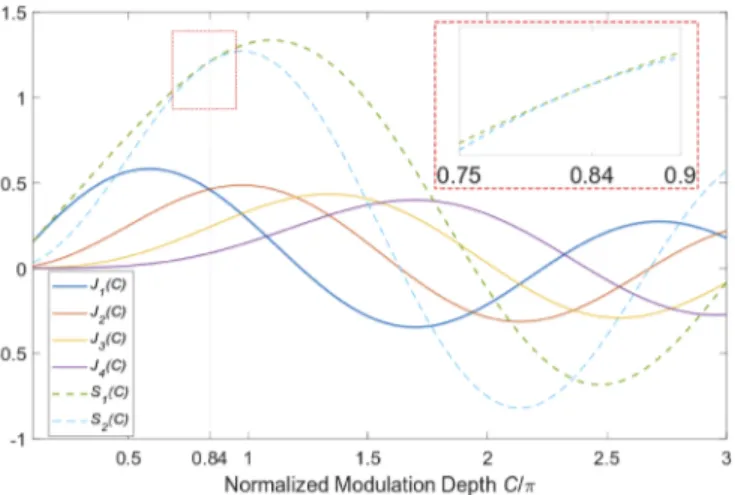
2[Ji−1(C) − Ji+1(C)]. (10) For the nominal modulation depth of C= 0.84π, the solution of (9) is a2= 2.5806 and

a3= −3.0339, but the equation can be solved for other nominal modulation depths as well. In

Fig.1we show the profiles of functions S1(C) and S2(C), together with the Bessel functions. It

is clear that at the nominal C, S1and S2not only are equal but also are their slopes, as imposed

by (8.b).

Now, we can calculate the phase from the ratio of the mixing with functions f1and f2:

∆φ_MTM(t)= arctan(︃ I ⊗ f1 I ⊗ f2 )︃ = arctan(︃ S1(C) sin ∆φ(t) S2(C) cos ∆φ(t) )︃ . (11)

The signal from (11) can also be approximated to the sum of the signal of interest and a non-linear component, as in (4), except in this case the distortion coefficient, now called υMTM,

will be determined by the variation of the quotient S1/S2as:

υMTM= ⎧ ⎪ ⎪ ⎨ ⎪ ⎪ ⎩ J1(C)−a3J3(C) a2J2(C) C ≠ 0.84π 1 C= 0.84π (12)

This coefficient will undergo a much smaller variation when C deviates from the nominal value, because its first derivative with respect to C is imposed to be zero, as can be seen in Fig.1.

Fig. 1. First four Bessel functions of the first kind and coefficients S1and S2versus the normalized modulation depth C/π for the case up to 3ω, and the nominal modulation depth C= 0.84π. J1and J₂have the same the value but not the same slope, while S₁and S₂have the same value and slope.

2.2. MTM up to 4ω

It is possible to make the PGC-MTM algorithm even more insensitive to the value of the modulation depth by considering f2(t)= a2cos 2ωt+ a4cos 4ωt, with a4≠ 0. After mixing and low-pass filtering, the following signals are obtained:

I ⊗ f1 = [a1J1(C) − a3J3(C)] sin ∆φ(t)= S1(C) sin ∆φ(t), (13.a)

I ⊗ f2= [a2J2(C) − a4J4(C)] cos ∆φ(t)= S2(C) cos ∆φ(t), (13.b)

In this case, having an extra parameter allows us to apply a third condition; therefore, besides making the functions and their first derivatives equal in C, we will force the second derivative to be the same too, which will increase the distortion-free range even further. The conditions are mathematically described below:

S1= S2(C), (14.a)

S1′= S2′(C), (14.b)

S1′′(C)= S2′′(C), (14.c)

these three equations, when written in matrix form, considering a1= 1, become:

⎛ ⎜ ⎜ ⎜ ⎜ ⎝ J3(C) J2(C) −J4(C) J′₃(C) J′₂(C) −J′₄(C) J′′₃(C) J′′₂(C) −J′′₄(C) ⎞ ⎟ ⎟ ⎟ ⎟ ⎠ ⎛ ⎜ ⎜ ⎜ ⎜ ⎝ a3 a2 a4 ⎞ ⎟ ⎟ ⎟ ⎟ ⎠ = ⎛ ⎜ ⎜ ⎜ ⎜ ⎝ J1(C) J′₁(C) J′′₁(C) ⎞ ⎟ ⎟ ⎟ ⎟ ⎠ . (15)

Solving (15) for the nominal case C= 0.84π, we find the solutions a2= 4.1936, a3= −9.7109

and a4= −9.8913. In this case we have a distortion parameter υMTMequal to:

υMTM = ⎧ ⎪ ⎪ ⎨ ⎪ ⎪ ⎩ J1(C)−a3J3(C) a2J2(C)−a4J4(C) C ≠ 0.84π 1 C= 0.84π . (16)

Figure2shows the variation of the distortion parameter υ versus variations of the modulation depth with respect to the nominal value, when the standard PGC and the MTM approach up

to 3ω and up to 4ω are applied. It is clear that both MTM methods are much more robust to modulation depth variations; in particular, the case up to 4ω has an even wider range, as expected, due to the extra condition cancelling the second derivative υ’’(C).

Fig. 2. Plot of the distortion parameter υ versus the normalized modulation depth C/π for

standard PGC (PGC-std), PGC-MTM up to 3ω and PGC-MTM up to 4ω.

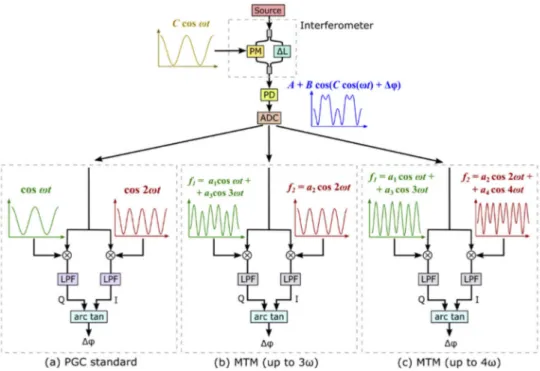
Fig. 3. Interferometer with PGC active phase demodulation using three techniques: (a)

Standard PGC, (b) MTM up to 3ω, (c) MTM up to 4ω. (b) and (c) are the schemes proposed in this work. The waveforms shown are the solutions for the nominal modulation depth C= 0.84π. MTM: Multitone mixing, PM: Phase modulator, PD: photodiode, ADC: analog-to-digital converter, LPF: low-pass filter, ∆L: path length difference between the interferometer arms.

Figure3shows a system consisting of an interferometer with active phase demodulation using three different PGC schemes: the standard PGC (Fig.3(a)), the MTM up to 3ω (Fig.3(b)) and up to 4ω (Fig.3(c)). The waveforms shown correspond to the specific solutions for the aicoefficients

at the nominal modulation depth C= 0.84π. Particularly, this figure shows a Mach-Zehnder interferometer, but the method can be applied to other types of interferometers, such as the Michelson.

3. Performance analysis

In order to test the method and quantitatively calculate the performance in terms of distortion and noise, we apply the method to a simulated interferometer signal with a sinusoidal waveform in presence of Gaussian noise. The signal on the sensing branch of the interferometer is:

∆φ(t) = D cos 2πf_pt+ φ0, (17)

with frequency fp= 120 Hz, amplitude D = 5 rad, and initial phase φ0=π/4. A strong signal

amplitude was selected to better appreciate the distortion effect, since this would be negligible for a small signal. The phase φ0was centered at π/4 because at this position the noise in the

in-phase and quadrature components have an equal contribution. Considering this input, we simulated the following intensity signal detected by the photodiode:

I= A + Bcos [Cmodcos(2πfmodt)+ D cos(2πfpt)+ φ0]+ Inoise, (18)

where we assumed A= B=1/2, fmod= 10 kHz, and in Inoisewe introduced a white noise with

standard deviation σnoise= 0.01. The resulting signal was processed as explained in the previous

section, mixing with multiples of fmodand low-pass-filtered with a bandwidth of 4kHz.

To measure and compare the performance of the PGC algorithms we calculated the total harmonic distortion (THD), defined as the ratio between the equivalent root-mean-square amplitude of all the harmonics and the amplitude of the fundamental frequency of the demodulated signal, expressed as [20]: THD = √︂ ∑︁∞ k=2Vk2 V1 , (19)

where V1 is the amplitude of the fundamental harmonic and Vk is the amplitude of the kth

harmonic. We also compare the performance in terms of the signal-to-noise and distortion ratio (SINAD), defined as the ratio between the power of the fundamental frequency, PS, and

the sum of the power of the additive noise, PN, and distortion components (harmonics) of the

demodulated signal, PD, expressed as [21]:

SINAD = PS

PN+ PD

. (20)

While THD quantifies the effect of the modulation depth deviation on the distortion of the demodulated signal, SINAD not only measures the effect of the distortion, but also considers the effect of the presence of noise in the demodulated signal.

Figure4shows the results for a nominal modulation depth of Cnom= 0.84π, which is the typical

value in the standard PGC. For the THD results, the first thing we can see in Fig.4(a) is that when

Cmod= 0.84π the THD is zero, meaning there is no distortion for any of the algorithms, since in

this case the value of υ in (4) is one, cancelling the non-linear term. When the deviation of Cmod

from the nominal value increases, so does the THD for all the PGC methods; however, since the variation of υ with respect to Cmodis much larger for PGC-std than for the proposed algorithms

(see Fig.2), its THD is also higher compared to PGC-MTM up to 3ω and PGC-MTM up to 4ω, therefore the proposed algorithms are more robust to modulation depth deviations. Regarding

the SINAD, we can see in Fig.4(b) that for the ideal case in which Cnom= Cmod= 0.84π the

value is slightly higher for PGC-std, at 107.1 dB, than for PGC-MTM up to 3ω, however as the deviation of the modulation depth from the nominal value increases, the SINAD for PGD-std rapidly decreases, whereas for PGC-MTM up to 3ω it remains at ∼106 dB for Cmodbetween

∼0.82π and ∼0.85π, therefore in this range this algorithm is less noisy than PGC-MTM up to 4ω, with a SINAD of ∼102 dB. The reason why the SINAD is almost flat for PGC-MTM up to 3ω in this range is that the SINAD considers both noise and distortion, hence close to the nominal point (Cnom= 0.84π), noise, which is a constant value, dominates, thus the flat top. At a certain point,

distortion starts to dominate, since, as it can be seen in Fig.4(a), the total harmonic distortion increases rapidly as the modulation depth deviates from the nominal value, causing a sharp drop in the SINAD, which is then lower than for PGC-MTM up to 4ω, hence for cases in which the modulation depth deviation is small, it is better to use PGC-MTM up to 3ω, since it is more robust to noise effects than PGC-MTM up to 4ω, and it has a lower THD than PGC-std outside the nominal case.

Fig. 4. (a) Total harmonic distortion when C deviates from the nominal value Cnom= 0.84π, extracted from the simulated data, for the three described demodulation techniques: standard (blue), MTM up to 3ω (orange), and MTM up to 4ω (yellow). (b) Signal to noise and distortion ratio under the same conditions, introducing an artificial noise in the detected signal with σ=0.01.

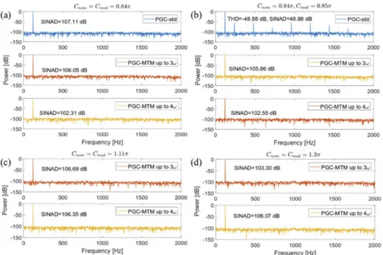
To further illustrate how distortion and noise affect the acquired signal, in Fig.5we show the power spectral density of the demodulated signals at different modulation depths. For Cnom=

Cmod= 0.84π there is no distortion for any of the PGC algorithms and we can see that the SINAD

is better for PGC-std, followed by PGC-MTM up to 3ω, as can be seen in Fig.5(a). However, a deviation of ∼1.2% from the nominal value of the modulation depth (Cmod= 0.85π) causes

visible distortion in PGC-std, as can be seen in Fig.5(b), resulting in a THD= −48.88 dB and SINAD= 48.88 dB, whereas there is still no distortion for the PGC-MTM algorithms. Figure5(b) also shows that in this case the SINAD is higher for PGC-MTM up to 3ω than for PGC-MTM up to 4ω, hence the former has a better performance.

Up until this point, we have evaluated the performance of the PGC-MTM algorithms for a nominal modulation depth of Cnom= 0.84π, but we can calculate the coefficients of the mixing

signals f1and f2for other nominal values (see sections2.1and2.2). Evaluating the SINAD for

different nominal modulation depths we found that for a value around Cnom= 1.11π the SINAD

for PGC-MTM up to 3ω and PGC-MTM up to 4ω is approximately the same, as can be seen in Fig.5(c), and if we further increase Cmodwe can reach a scenario in which the SINAD for the

method using up to 4ω is better than for up to 3ω, as can be seen in Fig.5(d), showing that in applications when the phase modulator can reach these high modulation depth values, we can

Fig. 5. Comparison of the spectrum between PGC-MTM up to 3ω and PGC-MTM up to 4ω

for: (a) Cnom=Cmod=0.84π and (b) Cnom=0.84π, Cmod= 0.86π, and between PGC-MTM up to 3ω and PGC-MTM up to 4ω for:(c) Cnom= Cmod= 1.11π, and (d) Cnom= Cmod= 1.3π.

obtain a better performance with PGC-MTM up to 4ω, that is comparable to the one obtained with PGC-std with Cnom= 0.84π.

In conclusion, these results show that at a nominal modulation depth of 0.84π, which is the one used in the standard PGC, the noise penalty of the MTM method up to 3ω with respect to the standard method is almost negligible (∼1 dB), while the MTM up to 4ω has a higher penalty (∼5 dB), which means that the MTM up 3ω is best suited for this modulation depth. However, if our modulator allows applying a higher modulation depth (between 1.11π and 1.3π), the noise penalty of the MTM up to 4ω becomes negligible, making it the best method in terms of distortion and noise.

4. Experiments and results

In this section we will show experimental results of the proposed MTM technique compared to the standard PGC scheme. The MTM method can be applied to a variety of interferometers in which the phase can be modulated externally. For instance, the phase can be modulated in one of the arms using a piezoelectric actuator, like in the case of some fiber-optic based interferometers (FOIs) [7], or through thermo-optic effect [22], carrier injection/depletion or other phase shifting mechanisms in photonic integrated circuit-based interferometers. The method can also be applied modulating the wavelength of the optical source [23], but in this case the interferometer must be unbalanced, so that wavelength changes are converted into phase variations.

4.1. Integrated interferometer design

The homodyne interferometer used for the experimental demonstration of the PGC-MTM technique was an integrated unbalanced Mach-Zehnder interferometer (MZI) on silicon-on-insulator (see Fig.6). The device, fabricated at CEA-Leti with deep-UV lithography, consists of

two MZIs, one with path length difference ∆L= 118.6 µm and FSR of 4.8 nm (600 GHz), so-called coarse, and another with ∆L= 948.7µm and FSR of 595 pm (75 GHz), so-called fine, which share the same input vertical grating coupler through a 2-by-2 multimode interference (MMI) coupler. The shorter arm of each MZI included a phase modulator based on the thermo-optic effect, consisting of a metal Ti/TiN heater track with length of 86 µm and width of 1.43 µm, characterized by a V2πof 3.69 V, and a 1/e time constant of 7 µs. Each MZI has an output grating

coupler for coupling to external photoreceivers. For the experiments we only used the fine MZI since it provides a higher resolution than the coarse [22].

Fig. 6. Optical microscope image of the integrated unbalanced MZI. The total footprint is

1430µm×400µm. The fine MZI, which is the one used in this paper, is located at the top, while the coarse MZI is at the bottom. GC: grating coupler.

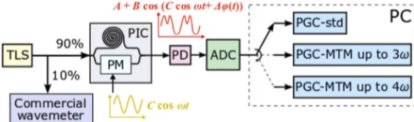
4.2. Experimental setup

The schematic of the experimental setup is shown in Fig.7. In this configuration the integrated unbalanced MZI is employed as a wavemeter to measure a wavelength shift generated using a tunable external cavity laser model EXFO T100S-HP (output power set to 10mW). In order to apply the PGC algorithms the phase modulator of the MZI was driven using the square-root of a sinusoidal signal at 1 kHz, since the power on the thermal phase shifter is proportional to the square of the applied voltage. The output of the interferometer was coupled to an external InGaAs-based amplified photoreceiver with a responsivity of ∼5·104V/W and a 775 kHz bandwidth. The traces were collected with a 16-bit data acquisition card model MCDAQ USB-1608FS at 100kS/s. Additionally, we compared the measurements with the commercial wavemeter model I-MON 512 USB from Ibsen Photonics A/S.

Fig. 7. General PGC schematic for demodulating the output of an integrated MZI. TLS:

tunable laser; PM: phase modulator; PD: photodetector; ADC: analog-to-digital converter; LPF: low-pass filter.

4.3. Results

To compare the performance of the different PGC algorithms when the modulation depth deviates from the nominal case of Cnom= 0.84π, we measured a wavelength shift from ∼1560 nm to

arms of the MZI. Figure8(a) shows the demodulated traces in the whole measuring range and Fig.8(b) shows a zoom of the measurement. In the latter it can be appreciated that the PGC-std algorithm has visible non-linearities in the form of an undulation that occurs every π/2 shift, or every quarter of the free spectral range of the MZI, whereas for PGC-MTM up to 3ω and up to 4ω there are no visible non-linearities when compared to the trace obtained with the commercial wavemeter, demonstrating the robustness of the PGC-MTM algorithms to modulation depth deviations.

Fig. 8. Comparison of the results of the wavelength shift measurement between PGC-std, the

proposed PGC-MTM algorithms and a commercial wavemeter (Ibsen) when Cnom= 0.84π and Cmod=0.97π. (a) View of the whole wavelength sweep. (b) Zoom of the measurement where it can be appreciated the non-linearity in the result of the PGC-std, which is absent in the traces obtained using the PGC-MTM algorithms and the commercial wavemeter.

In order to compare the noise levels for the different demodulation schemes, we measured the standard deviation of the signal when the wavelength was fixed. In Figs.9(a)-(c) we show the noise traces for the standard, MTM up to 3ω, and MTM up to 4ω techniques respectively, for the case in which Cnom= Cmod= 0.84π, which yielded the minimum noise for PGC-std. From

these figures, the standard deviation of the standard and MTM up to 3ω are very similar, 0.1175 pm and 0.1198 pm, respectively, while the MTM up to 4ω yielded a higher noise of 0.1277

Fig. 9. Comparison of the noise level of the demodulated signals with a 400 Hz bandwidth

for Cnom=Cmod=0.84π with (a) PGC-std, (b) PGC-MTM up to 3ω and (c) PGC-MTM up to 4ω, and for Cnom=Cmod=1.31π with (d) PGC-MTM up to 3ω and (e) PGC-MTM up to 4ω.

pm. An increase in noise with the MTM up to 4ω at this modulation depth was predicted in the previous section. However, the amount of the increase of noise is lower in the experiment than in the simulation (Fig.4(b) shows ∼5dB noise penalty); we attribute this to the contribution of wavelength noise of the source itself, which was not considered in the simulation.

On the other hand, Figs.9(d) and (e) show the experimental noise levels when the nominal modulation depth is increased to Cnom= Cmod= 1.31π, showing that the noise of the MTM up to

4ω technique is reduced again (down to 0.1002 pm), as predicted from the simulation results shown in Fig.5(d).

These results provide experimental evidence of the fact that distortion can be strongly reduced with the MTM technique, and that the noise does not increase significantly for the MTM up to 3ω with respect to the standard PGC technique, at Cnom= 0.84π, and neither for the even more

robust MTM up to 4ω when a higher modulation depth is applied.

5. Conclusion

We proposed and demonstrated a novel active phase demodulation technique for optical inter-ferometers which strongly reduces distortion under deviations of the modulation depth. The technique, called multitone mixing, consists of mixing the output waveform with linear combi-nations of even and odd harmonics of the modulating frequency, and choosing the coefficients to cancel the first and optionally the successive derivatives of the distortion parameter υ. The technique has several advantages with respect to previously proposed solutions, in particular, it provides the DC component of the phase, and it does not require signal variations, ellipse fitting algorithms, or recording previous data to correct distortion. We showed through simulations that when the nominal modulation depth is 0.84π, a deviation of ∼1.2% from this value causes visible distortion in PGC-std, resulting in a total harmonic distortion of −48.88 dB and SINAD of 48.88 dB, whereas the PGC-MTM algorithms did not show distortion. The calculated SINAD for PGC-MTM up to 3ω was 105.86 dB, whereas for PGC-MTM up to 4ω was 102.55 dB, hence the former has a better performance for this nominal modulation depth. However, for modulation depths higher than ∼1.11π MTM up to 4ω has a higher SINAD than MTM up to 3ω, making the former the best method in terms of distortion and noise in this range. The technique was also experimentally validated with a wavelength metering integrated interferometer and did not show a significant noise penalty with respect to the standard PGC technique.

Funding

Agenzia Spaziale Italiana; Regione Toscana.

Acknowledgements

This research was partially funded by Tuscany Region through a POR FESR Toscana 2014–2020 grant in the context of the project SENSOR, and by ASI (Italian Aerospace Agency) through the initiative “Nuove idee per la componentistica spaziale del futuro TRL”.

Disclosures

Y.M., P.V. and C.J.O. have filed a patent application with the idea proposed in this work (P).

References

1. M. D. Todd, G. A. Johnson, and C. C. Chang, “Passive, light intensity-independent interferometric method for fibre Bragg grating interrogation,”Electron. Lett.35(22), 1970–1971 (1999).

2. A. D. Kersey, T. A. Berkoff, and W. W. Morey, “High-resolution fibre-grating based strain sensor with interferometric wavelength-shift detection,”Electron. Lett.28(3), 236–238 (1992).

3. D. A. Jackson, A. D. Kersey, M. Corke, and J. D. C. Jones, “Pseudoheterodyne detection scheme for optical interferometers,”Electron. Lett.18(25-26), 1081–1083 (1982).

4. M. Song, S. Yin, and P. B. Ruffin, “Fiber Bragg grating strain sensor demodulation with quadrature sampling of a Mach–Zehnder interferometer,”Appl. Opt.39(7), 1106–1111 (2000).

5. A. Dandridge, A. B. Tveten, and T. G. Giallorenzi, “Homodyne Demodulation Scheme for Fiber Optic Sensors Using Phase Generated Carrier,”IEEE J. Quantum Electron.18(10), 1647–1653 (1982).

6. L. Wang, M. Zhang, X. Mao, and Y. Liao, “The arctangent approach of digital PGC demodulation for optic interferometric sensors,” in Interferometry XIII: Techniques and Analysis, (2006).

7. J. He, L. Wang, F. Li, and Y. Liu, “An Ameliorated Phase Generated Carrier Demodulation Algorithm With Low Harmonic Distortion and High Stability,”J. Lightwave Technol.28(22), 3258–3265 (2010).

8. A. Zhang and S. Zhang, “High Stability Fiber-Optics Sensors with an Improved PGC Demodulation Algorithm,” IEEE Sens. J.16(21), 7681–7684 (2016).

9. G. Q. Wang, T. W. Xu, and F. Li, “PGC demodulation technique with high stability and low harmonic distortion,” IEEE Photonics Technol. Lett.24(23), 2093–2096 (2012).

10. S. Zhang, Y. Chen, B. Chen, L. Yan, J. Xie, and Y. Lou, “A PGC-DCDM demodulation scheme insensitive to phase modulation depth and carrier phase delay in an EOM-based SPM interferometer,”Opt. Commun.474, 126183

(2020).

11. H. A. Deferrari, R. A. Darby, and F. A. Andrews, “Vibrational Displacement and Mode-Shape Measurement by a Laser Interferometer,”J. Acoust. Soc. Am.42(5), 982–990 (1967).

12. O. Sasaki and H. Okazaki, “Sinusoidal phase modulating interferometry for surface profile measurement,”Appl. Opt.

25(18), 3137 (1986).

13. Y. Tong, H. Zeng, L. Li, and Y. Zhou, “Improved phase generated carrier demodulation algorithm for eliminating light intensity disturbance and phase modulation amplitude variation,”Appl. Opt.51(29), 6962–6967 (2012).

14. V. S. Sudarshanam and K. Srinivasan, “Linear readout of dynamic phase change in a fiber-optic homodyne interferometer,”Opt. Lett.14(2), 140 (1989).

15. A. V. Volkov, M. Y. Plotnikov, M. V. Mekhrengin, G. P. Miroshnichenko, and A. S. Aleynik, “Phase Modulation Depth Evaluation and Correction Technique for the PGC Demodulation Scheme in Fiber-Optic Interferometric Sensors,”IEEE Sens. J.17(13), 4143–4150 (2017).

16. Z. Qu, S. Guo, C. Hou, J. Yang, and L. Yuan, “Real-time self-calibration PGC-Arctan demodulation algorithm in fiber-optic interferometric sensors,”Opt. Express27(16), 23593 (2019).

17. S. Zhang, B. Y. L. Chen, and Z. Xu, “Real-time normalization and nonlinearity evaluation methods of the PGC-arctan demodulation in an EOM-based sinusoidal phase modulating interferometer,”Opt. Express26(2), 605–616 (2018).

18. J. Xie, L. Yan, B. Chen, and Y. Lou, “Extraction of Carrier Phase Delay for Nonlinear Errors Compensation of PGC Demodulation in an SPM Interferometer,”J. Lightwave Technol.37(13), 3422–3430 (2019).

19. M. Abramowitz and I. A. Stegun, Handbook of Mathematical Functions, With Formulas, Graphs, and Mathematical Tables(Dover Publications, Inc., 1972), p. 361.

20. D. Shmilovitz, “On the definition of total harmonic distortion and its effect on measurement interpretation,”IEEE Trans. Power Delivery20(1), 526–528 (2005).

21. P. M. Lavrador, N. B. de Carvalho, and J. C. Pedro, “Noise and distortion figure - an extension of noise figure definition for nonlinear devices,” in IEEE MTT-S International Microwave Symposium Digest, Philadelphia, (2003). 22. Y. E. Marin, A. Celik, S. Faralli, L. Adelmini, C. Kopp, F. D. Pasquale, and C. Oton, “Integrated Dynamic Wavelength Division Multiplexed FBG Sensor Interrogator on a Silicon Photonic Chip,”J. Lightwave Technol.37(18), 4770–4775

(2019).

23. T. R. Christian, A. Frank, and B. H. Houston, “Real-time analog and digital demodulator for interferometric fiber optic sensors,” in Smart Structures and Materials 1994: Smart Sensing, Processing, and Instrumentation, 2191, Orlando, FL, United States, (1994).