Interferenze con la tradizione e intertestualità in Yoko Tawada e Emine Sevgi Özdamar

Università Degli Studi Di Salerno

Dipartimento di Fisica “E.R. Caianiello”

Dottorato di Ricerca in Matematica, Fisica e Applicazioni

Curriculum:

FISICA

XXX Ciclo – II Serie

2014-2017

Low and high field

Magnetic Resonance Imaging

and its application in food science and plants

Cristina Ripoli

Tutor : PhD Coordinator :

1

Index

Index 1

Introduction 4

1. Principles of Nuclear Magnetic Resonance 7

1.1 A mix description 7

1.2 Net Magnetization and Boltzmann distribution 12

1.3 Excitation and Bloch equations 15

1.4 Relaxation 18

1.4.1 Spin-lattice and spin-spin relaxation 20

1.5 Signal detection 23

2. Imaging by Nuclear Magnetic Resonance 26

2.1 Spatial encoding 27

2.1.1 Readout signal and k-space 33

2.2 Image contrast 34

2.3 Sequences 36

2.3.1 Spin echo 37

2

2.3.3 Gradient echo 40

2.4 Single Voxel Spectroscopy 42

3. Experimental Setup 44 Magnet 45 3.1 Probes 47 3.2 Gradients 49 3.3 Nmr software 49 4. MRI Application 51 4.1 Medicine 51 4.2 Porous media 53 4.3 Engineering applications 54 4.4 Plants 55 4.5 Food 56

5. Application in food science 59

5.1 Moisture migration 60

5.2 Low field investigation on eggplants 61

5.3 High field experiment on pumpkin 64

5.4 1H MR imaging on pumpkin 67

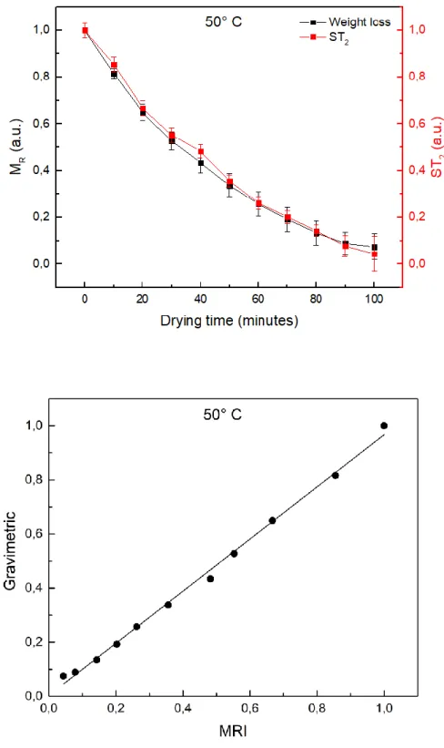
5.5 Results 71

5.6 Spectra 92

6. MRI of plants 105

6.1 Roots water uptake 105

6.2 Experiment 107

MRI protocol 108

3

Conclusion and future perspectives 120

List of acronyms 122

List of figures 124

4

Introduction

Nuclear Magnetic Resonance (NMR) and Magnetic Resonance Imaging (MRI) are techniques that have seen a remarkable success and a fast growth over the past decades.

These techniques, extensively used as survey and investigation tools in several fields, give usually a relatively rapid response, have a good level of accuracy and does not present the harmful disadvantages of other diagnostic approaches based on ionizing radiations.

In particular, MRI emerged as a medical imaging technique to obtain pictures of the anatomy and physiological processes of organs and body structures in both health and disease. Even if originally developed in the medical field, it is nowadays used in a large number of disciplines to study a wide variety of processes and materials.

MRI technique involves a nice combination of superconductivity, cryogenics, quantum physics, digital and computer technology.

Thanks to its non-invasivity and non-descrutivity, the MRI enhances its potential to perform inspections and studies of the internal structure of material samples without modifications caused by the measurements.

In particular, in the field of food science, the understanding of global information about the food matrix and a better identification of the determinants characterizing food quality and safety represent a new challenge and MRI has proven to be a very promising answer.

This technique can be used to acquire 2-dimensional (2D) and 3-dimensional (3D) high spatial resolution images of the internal structure of the material under study. The signal of each voxel depends on the physical properties of the sample such as proton density, relaxation times, temperature and diffusion.

5

Information extracted from the images can be exploited for spatially resolved measurements of concentration, structure, temperature, velocity, and diffusivity.

MRI, as non-destructive technique, allows the study of intact samples such as fruits and vegetables. Due to the presence of a high water content in these products, MRI can be useful to obtain information about tissue properties and, thanks of its sensitivity, can trace water distribution and migration.

MRI shows a great potential for the investigation of the structural changes induced by food processes and allows the characterization of vegetable and plant structure. The characteristic NMR relaxation times are used as parameters for the quantification of water content or for the extraction of information related to changes in microstructure.

Nevertheless, the way to affirm the MRI as a recognized tool for the assessment of food properties, quality, processing and storage is still quite long and the implementation of simple and fast protocols, suitable to respond to food industry demands, is far to be reached. The idea behind this thesis is the investigation of new methodologies intended to carry out fast and accurate evaluation of moisture content in a food matrix through MRI. At the same time the development of appropriate protocols and analysis tools allowing a simple extraction of those information in a reproducible and reliable way.

This thesis work is divided into six chapters.

Chapter 1 and 2 offer a general introduction respectively to the NMR physics and to the imaging technique based on it. In particular, the processes behind the image formation and the used sequences are discussed.

A general description of the instrument is presented in chapter 3.

Chapter 4 provide a short overview of the most prominent applications of MRI and the state of the art in various fields of use.

In chapter 5, we explain our advances in efforts to develop an objective, accurate and non-invasive tool for the detection and quantification of the moisture content in a specific food matrix. Two different approaches have been used, both based on data extracted by MR Imaging and a comparison of the two methods is presented. The goal is to exploit MRI as a real measurement instrument with a simple and

6

fast measurement protocol: to achieve this goal we need to identify quantitative MR parameters that provide the most relevant information with respect to the physical quantities we want to measure.

The final chapter describes a preliminary MRI study of in vivo monitoring of plants behaviour and their growing inside the spectrometer. The determination of roots viability, water uptake and absorption of nutrients can be explored through MRI in a continuous way with very light interference on the plant development. The first results and the perspectives of this kind of studies are presented.

The thesis ends with a general conclusion where are summarized the main results and the key perspectives for future work.

7

1. Principles of Nuclear Magnetic Resonance

The Nuclear Magnetic Resonance (NMR) is a quantum mechanical phenomenon in nature, but at the macroscopic scale, it is possible to describe it quite accurately using semi-classical physics. This point of view allows having a practical and simpler approach to understand the NMR phenomenon.

1.1 A mix description

Electrons, protons and neutrons are particles inherently provided with spin, characterized by quantum behaviour. The angular momentum associated with the spin is:

𝐿 = ℏ √𝐼(𝐼 + 1) ; ℏ = ℎ 2𝜋 ,

(1)

where I is the spin number and ℎ = 6,63 10−34 _𝐽𝑠2 _{is the Plank constant.}

For nuclei possessing an odd mass number, I value is a half-integer, like the hydrogen (1H) which possess a spin of +1/2 (Table 1).

8

Table 1 Spin quantum numbers for some nuclei.

The components measured along the axis are quantized. The quantum number 𝑚 may have only (2I + 1) value and may be any one of a discrete set of integer or half-integer values in the range:

𝑚𝐼= 𝐼, 𝐼 − 1, … . . , −𝐼 , (2)

that correspond to the basis states of the particles.

Atomic nuclei have a magnetic dipole moment proportional to the angular momentum:

𝜇⃗ = 𝛾 𝐿⃗⃗ = 𝛾 ℏ 𝐼⃗ . (3)

The constant of proportionality is the gyromagnetic ratio, γ, it is the ratio of the magnetic moment to the angular momentum and it depends on the considered nuclei, for the proton 𝛾_𝑃 = 268 𝑀𝐻𝑧/𝑇. The gyromagnetic ratio over 2π, gives

most common value used in NMR: 𝛾𝑃= 42,56 𝑀𝐻𝑧/𝑇.

The component of the angular momentum and the corresponding magnetic moment along the z-axis are respectively given by:

𝐿𝑧 = ℏ 𝑚𝐼 ; 𝜇𝑧 = 𝛾 ℏ 𝑚𝐼 . (4)

Applying an external magnetic field 𝐵⃗⃗ the interaction energy of a magnetic dipole 𝜇⃗ with the field is:

9

The consequence is the splitting of the energy levels that occurs because of the interaction of the magnetic moment ⃗⃗⃗ of the atom with the magnetic field 𝐵⃗⃗, slightly shifting the energy of the atomic levels.

Considering 𝐵⃗⃗ oriented on the z-axis,𝐵⃗⃗₀ = 𝐵₀𝑘̂, the (5) reduces to:

𝐸𝐼= −𝜇𝑧𝐵0= −𝛾 ℏ 𝑚𝐼𝐵0 (6)

Remembering that for the proton I=1/2, along the z-axis, m can only result in two values:

𝑚𝐼= 1 2⁄ , − 1 2⁄ (7)

The only two possible energy states for the spin proton are:

𝐸 = { 𝐸1 2⁄ = − 1 2𝛾ℏ𝐵0 𝐸−1 2⁄ = 1 2𝛾ℏ𝐵0 . (8)

The splitting of energy levels due to an external magnetic field is the so-called

Zeeman effect. In the absence of 𝐵⃗⃗₀, the two energy levels are degenerate. The two energy levels for the proton correspond to the two discrete values of I (Figure 1).

10

The proton can swap between the two states simply by gaining or losing a certain amount of energy in the form of a photon. The spin-up state has less energy than the spin-down state:

𝐸1 2⁄ < 𝐸−1 2⁄ (9)

The lower energy level occurs when the proton magnetic moment component and the external magnetic field are parallel while, a higher energy level is obtained if they are anti-parallel. The energy separation between the levels is always 𝛾ℏ𝐵₀, for the proton difference in energy ∆E between these two levels is:

∆𝐸 = 𝐸−1 2⁄ − 𝐸1 2⁄ = 𝛾ℏ𝐵0 = 2𝜇𝐵0 (10)

From the quantic point of view, not only spin angular momentum, but also the transfer of energy, may assume only discrete unit, such a transition can be caused by a photon of light whose frequency, ν, is related to the energy gap, ∆𝐸, between the two levels according to:

∆𝐸 = ℎ 𝜈 = ℏ𝜔, (11)

where ω is called resonance frequency ωR.

Comparing the latter equation and the Zeeman equation (10) it is possible to find:

𝜔𝑅=

∆𝐸

ℏ = 𝛾𝐵0 .

(12)

11

The energy required to the transition from one energy state to the other, corresponds to an electromagnetic wave with an energy ∆𝐸 and a frequency 𝜔_𝑅 proportional to the magnetic field 𝐵⃗⃗₀. The increasing of the magnetic field get a greater resonance frequency.

At the same time, considering the classical description, the proton spin will tend to precess around the magnetic field with a frequency traditionally called the Larmor frequency, ω⃗⃗⃗_L.

Figure 3 Precession of a nucleus.

When the proton interacts with the external magnetic field, B⃗⃗⃗₀ = B₀k̂, it experiences a torque given by:

𝜏⃗ = 𝜇⃗ ∧ 𝐵⃗⃗0 . (13)

This torque acts to rotate the magnetic moment vector of a proton to align it with the external magnetic field. Using the cardinal equation of dynamics:

𝜏⃗ =𝑑𝐿⃗⃗ 𝑑𝑡 ,

(14)

and replacing (3) and (14), follow:

𝑑𝜇⃗

12

The Larmor frequency can be visualized classically in terms of the precession of the magnetic moment around the magnetic field:

𝜔⃗⃗⃗𝐿= −𝛾𝐵⃗⃗0. (16)

The minus sign is there to make sure that ω⃗⃗⃗_L defines a clockwise rotation about the z-axis.

The resonance frequency and the Larmor frequency are the same:

𝜔𝐿 = 𝜔𝑅 , (17)

this is the principal result about the NMR phenomenon.

The link between the classical and quantum mechanical is clear, the precessional frequency of the proton in a magnetic field is the same as the frequency of radiation required to cause transitions between two states.

This is not a rigorous derivation from quantum mechanics but does show how directly the Larmor relation results from very basic concepts. The fact that Planck's constant disappears from the solution implies that a non-quantum explanation using classical physics is possible [1].

Applying a transverse RF wave at the Larmor frequency (usually in the 10 to 103 MHz range) nuclear spins are excited. Successively they return to the lower energy state emitting an electromagnetic wave that can be detected.

1.2 Net Magnetization and Boltzmann distribution

In a macroscopic sample there is a larger number of spins, so it is necessary to use the methods of Statistical Physics and to introduce the macroscopic magnetization. Under the hypothesis of non interacting protons, all of them add up their magnetic moment to the net magnetization M⃗⃗⃗⃗.

Instead of using the individual nuclear spins, it is possible to use M⃗⃗⃗⃗, which can be treated as a vector of the classical physics.

13

In the absence of the external magnetic field (B⃗⃗⃗₀ = 0) there is no preference for ‘spin up’ or ‘spin down’ states, the magnetic dipoles are oriented randomly and there is no net magnetization (M⃗⃗⃗⃗ = 0).

For a population of spins with I = 1/2, only the two spin states are allowed:  μ⃗⃗ parallel to B⃗⃗⃗₀ (m = +1/2)

 μ⃗⃗ antiparallel to B⃗⃗⃗0 (m = -1/2)

Applying an external magnetic field the magnetic moments of the nuclei can align either parallel to the field (lower energy) or antiparallel (higher energy). The two energy levels are respectively referred to “spin-up” (𝛼) and “spin-down” (β) states.

Figure 4 Boltzmann distribution, the net magnetization M0 is proportional to the population difference

(𝑁 𝛼− 𝑁𝛽 ) and it is aligned exactly with the field.

Under thermal equilibrium conditions, these two energy levels are populated according to the Boltzmann probability distribution that describes the number of nuclei in each spin state:

𝑁𝛽

𝑁𝛼

= 𝑒∆𝐸 𝑘⁄ 𝐵𝑇_{= 𝑒}−𝜇𝐵0⁄𝑘𝐵𝑇 (18)

where 𝑁 α and 𝑁β represent the number of spins one would expect to respectively

measure in the spin-up and spin-down configurations, ΔE is the energy separation between the two states, kB= 1.381 x 10−23 J/°K is the Boltzmann constant

and T is the absolute temperature in Kelvin degrees.

At room temperature, the number of spins in the lower energy level, 𝑁_α , slightly outnumbers the number in the upper level, 𝑁 _β, only a small excess of spins can be expected to be found in the lower energy (spin-up) state when measurements

14

occurred. In presence of the main magnetic field 𝐵⃗⃗₀ = 𝐵₀𝑘̂, the net magnetization M0 is proportional to the population difference (𝑁 α− 𝑁β ) and it is aligned

exactly with the field (Figure 5), there is no net transverse component of M as the phase of the spins is randomly distributed.

Figure 5 The applied magnetic field causes an energy difference between aligned (𝛼) and unaligned (𝛽)

nuclei producing the net magnetization 𝑀⃗⃗⃗.

In a magnetic resonance experiment, the energy difference ΔE, between the two energy levels, is proportional to the field strength. Increasing the field strength there is an increasing of the energy difference and hence also of the population difference. Since the intensity of the NMR signal is directly dependent on the population difference, the signal also increases.

In principle to increase the spin polarization (population difference), there are two possibilities: either increase the external magnetic field or low the temperature. In practice, only the former way is exploited in NMR experiments.

For the majority of MR-experiments and for this thesis work, the proton (1H) is the nucleus of interest, because of its high natural abundance (Table 2) under the form of H2O in the biological samples. However, other nuclei such

15

Table 2 summarizes the NMR characteristics of the nuclei studied in vivo (Bernstein, et al., 2004 p. 960; de

Graaf, 2007 p. 9).

1.3 Excitation and Bloch equations

In the case of independent spins, it is possible to describe their motion in terms of the precession of the spins magnetization vector. By equating the torque to the rate of change of angular momentum, follow:

𝑑𝑀⃗⃗⃗

𝑑𝑡 = 𝛾𝑀⃗⃗⃗ ∧ 𝐵⃗⃗0 . (19)

The solution to equation (19), when B0 is a magnetic field, corresponds to a

precession of the magnetization, M⃗⃗⃗⃗0 = M0k̂, at the Larmor frequency ω0 = 𝛾𝐵0.

Remembering B⃗⃗⃗₀ = B₀k̂: 𝑑𝑀𝑥 𝑑𝑡 = 𝛾𝑀𝑦𝐵0 𝑑𝑀𝑦 𝑑𝑡 = −𝛾𝑀𝑥𝐵0 𝑑𝑀𝑧 𝑑𝑡 = 0 . (20) follow:

16

𝑀𝑥(𝑡) = 𝑀𝑥(0) 𝑐𝑜𝑠 𝜔0𝑡 + 𝑀𝑦(0) 𝑠𝑖𝑛 𝜔0𝑡

𝑀𝑥(𝑡) = −𝑀𝑥(0) 𝑠𝑖𝑛 𝜔0𝑡 + 𝑀𝑦(0) 𝑐𝑜𝑠 𝜔0𝑡

𝑀𝑧(𝑡) = 𝑀𝑧(0).

( 21)

To carry out an NMR experiment is necessary to apply a short burst of resonant RF field in order to disturb the spin system from the equilibrium.

Considering the circularly polarized component of a transverse time varying magnetic field 𝐵⃗⃗1, oscillating at 𝜔0, in the same sense as the spin precession, it is

possible to create a resonance phenomenon.

𝐵⃗⃗1(𝑡) = 𝐵1𝑐𝑜𝑠(𝜔0𝑡) 𝑖̂ − 𝐵1𝑠𝑖𝑛(𝜔0𝑡) 𝑗̂ . (22)

The Bloch equations become:

𝑑𝑀𝑥 𝑑𝑡 = 𝛾[𝑀𝑦𝐵0+ 𝑀𝑧𝐵1𝑠𝑖𝑛 𝜔0𝑡] 𝑑𝑀𝑦 𝑑𝑡 = 𝛾[𝑀𝑧𝐵1𝑐𝑜𝑠 𝜔0𝑡 − 𝑀𝑥𝐵0] 𝑑𝑀𝑧 𝑑𝑡 = 𝛾[−𝑀𝑥𝐵1𝑠𝑖𝑛 𝜔0𝑡 − 𝑀𝑦𝐵1]. (23)

Under the initial condition 𝑀⃗⃗⃗(𝑡) = 𝑀₀k̂ the solutions are:

𝑀𝑥(𝑡) = 𝑀0𝑠𝑖𝑛 𝜔1𝑡 𝑠𝑖𝑛 𝜔0𝑡

𝑀𝑦(𝑡) = 𝑀0𝑠𝑖𝑛 𝜔1𝑡 𝑐𝑜𝑠 𝜔0𝑡

𝑀𝑧(𝑡) = 𝑀0𝑐𝑜𝑠 𝜔1𝑡 ,

(24)

where ω₁ = 𝛾𝐵₁.

These equations imply that applying a rotating magnetic field of frequency ω0,

the magnetization simultaneously precess about the longitudinal polarizing 𝐵0 at

17

In the laboratory frame, the motion looks like a spiral since it is also precessing about the z-axis (Figure 6).

Figure 6 Laboratory frame:Evolution of the magnetitation in the presence of B0 and B1 (taken from [1] ).

At this point, it is helpful to make a coordinate transformation to a rotating frame (x’,y’,z’) at the Larmor frequency about the z-axis, which is defined by the direction of 𝐵₀. In this frame, the time dependence from the RF field B is rem oved and 𝐵₁ appear stationary.

The motion of the magnetization 𝑀⃗⃗⃗ in the new rotating frame at 𝜔 frequency can be described by: (𝑑𝑀⃗⃗⃗ 𝑑𝑡) 𝑟𝑜𝑡 = (𝑑𝑀⃗⃗⃗ 𝑑𝑡) 𝑓𝑖𝑥𝑒𝑑 − 𝜔⃗⃗⃗ ∧ 𝑀⃗⃗⃗ . (25)

Comparing this equation with the (19) it is possible to model the motion of the magnetization in the rotating frame by the same equation as in the fixed frame:

(𝑑𝑀⃗⃗⃗ 𝑑𝑡) 𝑟𝑜𝑡 = 𝛾𝑀⃗⃗⃗ ∧ (𝐵⃗⃗0+ 𝜔⃗⃗⃗ 𝛾) . (26)

The term ω γ⁄ represents a fictitious magnetic field due to the rotation. The new expression define a new effective field B⃗⃗⃗_e, experienced by the spins:

𝐵⃗⃗𝑒= (𝐵⃗⃗0+

𝜔⃗⃗⃗ 𝛾)

(27)

18

(𝑑𝑀⃗⃗⃗

𝑑𝑡)_𝑟𝑜𝑡= 𝛾𝑀⃗⃗⃗ ∧ 𝐵⃗⃗𝑒

(28)

So in the rotating frame, the magnetization precede about B⃗⃗⃗_e as shown in the picture (Figure 7):

Figure 7 Rotating frame: precession of the magnetization (taken from [1]).

When the frame rotates at ω⃗⃗⃗ = −γB⃗⃗⃗0, the effective field becomes zero and 𝑀⃗⃗⃗ is a

fixed vector in the rotating frame.

In the real systems the spins interaction have to be take into account.

1.4 Relaxation

When the RF pulse, used to excite the spin system, is over the system tends to recover its original repose state, there must subsequently be a process to restore the equilibrium. This involves the exchange of energy between the spin system and respectively its surroundings and among themselves. Both relaxations occur at the same time.

In the first case, the recovering of M0 to equilibrium means the restoration of the

state of polarization where M0 is directed along the longitudinal magnetic field B0,

this is the reason because of the process is alternatively named longitudinal relaxation. The phenomenological description of this process is defined in a new equation of motion for Mz:

19 𝑑𝑀𝑧 𝑑𝑡 = −(𝑀𝑧− 𝑀0) 𝑇1 (29)

where T1 is known as the spin-lattice or longitudinal relaxation time and the

solution of the (29) is:

𝑀𝑧(𝑡) = (0)𝑒−𝑡 𝑇⁄ 1+ 𝑀0 (1 − 𝑒−𝑡 𝑇⁄ 1). (30)

The process is known as spin-lattice relaxation.

In the second case the process that bring about the nuclear spins to thermal equilibrium among themselves is known as spin-spin relaxation and the time constant involves is called T2 spin-spin relaxation time or transverse relaxation

time (see section 1.4.1).

This phenomenon has a decreasing exponential behaviour described by the equations describingthe evolution of Mx and My:

𝑑𝑀𝑥,𝑦

𝑑𝑡 =

−𝑀𝑥,𝑦

𝑇2

(33)

where the solutions are:

𝑀𝑥,𝑦(𝑡) = 𝑀𝑥,𝑦(0)𝑒−𝑡 𝑇⁄2. (34)

Transverse magnetization corresponds to a state of phase coherence between the nuclear spin states. This means that transverse relaxation is sensitive to interaction terms which cause the nuclear spins to dephase [1].

If the system was initially in equilibrium and RF pulse was a 90° pulse applied along x’-axis: 𝑀𝑥(0) = 𝑀𝑧(0) = 0 ; 𝑀𝑦(0) = 𝑀0, (31) and 𝑀𝑧(𝑡) = 𝑀0(1 − 𝑒 −𝑡 𝑇1 ⁄ _). (32)

20

T2, while the z magnetization simply grows from zero back to M0.

In the rotating frame the Bloch equations become:

𝑑𝑀𝑥 𝑑𝑡 = 𝛾[𝑀𝑦𝐵0+ 𝑀𝑧𝐵1𝑠𝑖𝑛 𝜔0𝑡] − 𝑀𝑥 𝑇2 𝑑𝑀𝑦 𝑑𝑡 = 𝛾[𝑀𝑧𝐵1𝑐𝑜𝑠 𝜔0𝑡 − 𝑀𝑥𝐵0] − 𝑀𝑦 𝑇2 𝑑𝑀𝑧 𝑑𝑡 = 𝛾[−𝑀𝑥𝐵1𝑠𝑖𝑛 𝜔0𝑡 − 𝑀𝑦𝐵1] − (𝑀𝑧− 𝑀0) 𝑇1 . (35)

These set of differential equations describe the changes in the magnetization during excitation and relaxation and describe completely the main phenomena in NMR imaging using classical mechanics [1].

1.4.1 Spin-lattice and spin-spin relaxation

Spin-lattice relaxation

As mentioned before, the exchange of energy between the spin system and its surroundings is the so called spin-lattice relaxation. Since the magnetic field is applied to the sample until the thermal equilibrium is reached, the macroscopic magnetization experiments grow exponentially.

As spins go from a high energy state back to a low energy state, RF energy is released back into the surrounding lattice. The rate at which equilibrium is restored is characterized by the longitudinal relaxation time, T1. The recovery of

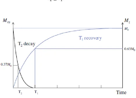
longitudinal magnetization follows an exponential curve (Figure 8).

The recovery rate is characterized by time constant T1 that represents the time

needed to recover the 63% of the longitudinal magnetization Mz.

It depends on the structure and molecular composition, the material state, viscosity and magnetic interactions. It has a lower value in solid than in a liquid state.

21

Figure 8 Spin- lattice relaxation (taken from [2]).

Spin-spin relaxation

The spin-spin relaxation is in general a faster process than spin-lattice relaxation and it is characterized by the spin-spin or transverse relaxation time, T2.

Transverse magnetization decay is described by an exponential curve characterized by the time constant T2 (Figure 9). Protons are influenced by

non-uniform, low magnetic fields produced by the near nuclei, which cause different speed precession. When the RF stops, the proton suffers a phase difference, Mxy

decreases and tend to zero. After time T2, transverse magnetization has reduce its

intensity of 37% of its original value. In the spin-spin interaction, the relaxation time T2 is independent of field strength.

22

Since the longitudinal magnetization cannot be restored, if the transverse magnetization does not disappear, T2 is always shorter than T1 (Figure 10). The

relation between the two time constants is:

𝑇2≤ 𝑇1. (36)

Figure 10 T1 and T2 relaxation occur simultaneously, the T2 decay is much quicker than the T1 recover

(taken from [2]).

In the hypothesis of interacting spins, the decay of the transverse magnetization is caused by the combination of two factors. It is necessary to take into account that in the Mxy decay the time constant T2 due to the molecular interactions is not the

only contribution but also the inhomogeneity due to B0 variations are

characterized by a time constant, T₂′.

The combination of these two factor gives the effective time constant of Mxy

decay called 𝑇₂∗ _{following the relation:}

1 𝑇₂∗= 1 𝑇2 + 1 𝑇₂′ . (37)

23

1.5 Signal detection

The equilibrium is characterized by a state of polarization with M0 directed along

the longitudinal magnetic field B0. M0 is a measurable magnetization of the order

of microtesla (μT), but smaller than the main magnetic field (T) so its detection results really difficult.

M0 becomes a significant signal, easier to record, simply tipping it in the

transverse plane (x-y) and detecting the induced voltage using a receiver coil which measures the magnetic fields only in this plane. To rotate the magnetization a 90° RF pulse is applied, this pulse tips M0 vector from the longitudinal plane

(parallel to B0) to the transverse plane (perpendicular to B0) where it can be

detected.

The semi-classical magnetization approach again gives a complete explanation of the process. The RF pulse creates a magnetic field within the transmit coil which is perpendicular to B0 and oscillating at the Larmor frequency (to respect the

resonance conditions).

In the rotating frame, this is the static field B1 aligned along x’ in the transverse

plane (Figure 11 a). M0 moves away from the z-axis until the RF pulse is switched

off (Figure 11 b). As seen in the previous section (Figure 6) the motion looks like a spiral since it is also precessing about the z-axis.

Figure 11 (a) The RF pulse produces a fixed magnetic field B1 in the rotating frame. (b) M0 precess about B1

until the RF is switched off (taken from [2]).

The RF pulse brings the spins into phase coherence consequently, M0 induce a

24

magnetization perpendicular to B0. In the laboratory frame, M0 is now precessing

in the transverse plane (Figure 12 a), so the coil sees an oscillating magnetic field which induces a voltage varying at the Larmor frequency.

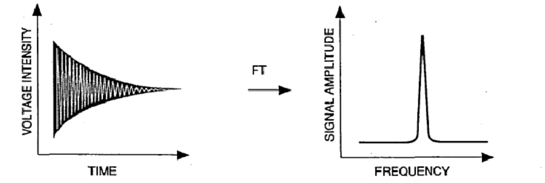
Since the protons rapidly dephase with respect to each other the amplitude of the signal decays exponentially to zero in only a few milliseconds (Figure 12 b). The free precession of magnetization induces a decaying signal known as Free

Induction Decay (FID) that is measured in the time domain and represent the

primary NMR signal.

Figure 12 (a) Precession on the flipped magnetization in the transverse plane. (b) FID- Signal induced in the

receiver coil (taken from [2]).

It is possible to represent this signal in the frequency domain through the Fourier transformations.

Figure 13 The FT process takes the time domain function (the FID) and converts it into a frequency domain

function (the spectrum).

Once all these signals are collected, the application of a Fourier transform converts the spatial frequency distribution into a spatial distribution of the excited nuclei.

25

The FID is never directly measured in a MRI experiments, what happens is described in the next chapter where the MRI principles will be described in detail.

26

2. Imaging by Nuclear Magnetic Resonance

The strength of the magnetic resonance imaging is to exploit linearly varying magnetic fields to enhance a spatial dependence.

Over the static field B0, that points in the longitudinal direction and the transverse

RF field B1 produced by coils tuned to the Larmor frequency, in MR imaging

there are three additional fields that vary spatially, the so called gradients.

The local frequency will vary with position by the linear relation between the Larmor frequency and the nuclear spin coordinates 𝑟⃗ , following the relation:

𝜔(𝑟⃗) = 𝛾(𝐵0+ 𝐺⃗ ∙ 𝑟⃗ ) , (38)

where G⃗⃗⃗ is defined in the usual manner as the grad of pulsed gradient field component parallel to 𝐵⃗⃗₀. This equation describes the frequency precession in presence of a gradient field. The first term comes from the static magnetic field but because of the presence of the gradient field, there is an additional term which adds another element to the Larmor equation that depends on the position.

This simple relation between the Larmor frequency and the nuclear spin coordinates 𝑟⃗ in the sample, lies the fundamental of the imaging principle; the resonance frequency of the magnetization will vary in proportion to the gradient field and this change in frequency can be used for spatial encoding.

27

2.1 Spatial encoding

Spatial encoding consist on successively applying magnetic field gradients. The magnetization precessing close to the resonance frequency is affected by the RF field whereas the pulse does not affect magnetization at distant frequencies. The RF pulse includes a set of frequencies centered on the Larmor frequency; this range of frequencies constitutes the RF bandwidth, ∆𝑓, (expressed in Hertz). In absence of the gradient fields, all the spins experience the same field B0 and

have the same frequency; the application of a gradient causes a protons frequency variation as a function of position along the direction of the gradient.

When a gradient is added for example, on the x direction, the resonance frequency varies with position and the magnetic field produced adds to the main field B0.

Along the x-direction, the MR signal shows higher or lower frequencies, which means that protons can resonate faster or slower depending on their precession position. In this way frequency measurements may be used to distinguish between MR signals at different positions in the space.

Figure 14 All the spins experience the same field and have the same frequency. When the gradient is added

moving along the x direction these protons resonate faster or slower depending upon their position. (Taken from [3].

The sets of gradients give MR its three dimensional capability. Firstly, a slice selection gradient (Gs) is used to select the volume of interest. Within this volume,

28

the position of each point will be encoded vertically and horizontally by respectively applying a phase encoding gradient (GΦ) and a frequency encoding

gradient (Gf). Magnetic field gradients form the basis of MR signal localization.

Slice selection

Through the selection gradient Gs ,applied in the z-direction, a selective excitation

of slice in the x-y plane is possible. The slice selection process is achieved by applying the RF pulse to tip the spins at the same time as the gradient.

The resonance frequency of the spins during the application of the z gradient becomes:

𝜔(𝑧) = 𝛾(𝐵0+ 𝐺𝑧𝑧 ). (39)

The RF excitation pulse contains a narrow range of frequencies centered about the Larmor frequency; at isocentre of the gradient (z = 0) where the effect of the gradient is zero, the frequency is: 𝜔 = 𝛾𝐵₀.

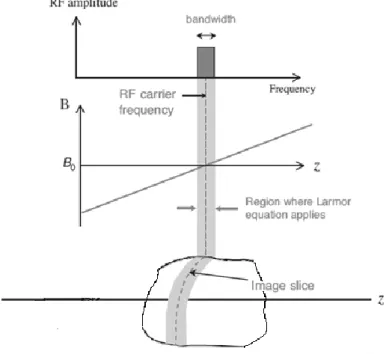
Modulating the RF envelope with a predetermined shape, for example a SINC shaped envelope pulse, a selective RF pulse is generated (Figure 15).

Figure 15 Slice selection gradient Gz (taken from [4]).

The excitation will take place only if the required frequency is present within the RF pulse’s transmit bandwidth (or close to the isocentre) otherwise the resonance does not happen and no MR signal is produced.

29

For extreme points along the gradient axis, in fact, the frequency required for resonance will not be present within the RF pulse bandwidth so no signal will be produced from these points. Only one slice remains selected. The slice-selection gradient translate the desired band of frequencies into the desired band of locations, corresponding to the slice [4].

Figure 16 Selective excitation of an image slice by applying a shaped RF pulse and a field gradient at the

same time.

The amplitude of slice selection gradient Gz and RF pulse bandwidth determine

the slice thickness. For a fixed RF bandwidth ∆𝑓, the increasing of the amplitude of the gradient correspond to a decreasing of the thickness of the slice.

As shown in the Figure 17, the slope of each of the two lines represents the strength of a slice selection gradient (Gz,1 and Gz,2). For a given ∆𝑓 of the RF

30

Figure 17 Larmor frequency versus position along the gradient direction , z-axis (taken from [4]).

By applying the selective gradient and changing the central frequency of the RF pulse it is possible to move the position of the slice. In this way it is possible to make multi-slices acquisitions.

The slice-select gradient is applied simultaneously to the RF pulse and it will not be on during the readout.

Phase encoding

The idea behind phase encoding is to create a linear spatial variation of the phase of the magnetization (the phase is the angle made by the transverse magnetization vector with respect to some fixed axis in the transverse plane). The phase encoding gradient, GΦ, is applied on the y-direction. It modifies the spin

resonance frequencies, inducing dephasing, which persists after the gradient is interrupted. This means that all the protons precess in the same frequency but in different phases: this phase difference lasts until the signal is recorded. The protons in the same row, perpendicular to the gradient direction, will all have the same phase (Figure 18).

31

Figure 18 Phase encoding. The arrows represent transverse magnetization at the center of each pixel.

At the end of the RF excitation pulse, the transverse magnetization has the same phase (direction) in each pixel (Figure 18 a). After a phase-encoding gradient is applied, the phase of the transverse magnetization varies at each location along the phase-encoded direction (Figure 18 b).

In principle, during the gradient pulse spins at different y locations precess at different frequencies, the spins precession will speed up or slow down according to their position along the y-axis. This causes the spins to dephase to a progressively greater degree as long as the gradient is applied, the relative phase shift is linear with y.

When the gradient is interrupted, all the spins come back to their original frequency, but keep their different phase angles, so they are phase encoded: in this way they can be localized on y-axis.

All of them precess in the same frequency but in different phases. This phase difference lasts until the signal is recorded. The MR signal is sampled after the gradient is turned off, so during the sampling there is no spread of frequencies due to the gradient; all the spins are precessing at 𝜔₀ = 𝛾𝐵₀.

The MR sequence consists of multiple repetitions of the excitation process followed by a different phase encode gradient until all possible spatial frequencies are interrogated, a RF pulse is required for every line of data. This is the reason because of in a pulse sequence diagrams the phase-encode steps are represented by a series of parallel lines (Figure 19).

32

Frequency encoding

Frequency-encoding of spatial position is accomplished through the use of a third magnetic field gradient, GF. Applying the frequency encoding gradient, the

Larmor frequency in the horizontal direction is modified becoming a function of the position and the x direction results encoded. It thus creates proton columns, which all have an identical Larmor frequency. The frequency encoding gradient is turn on during the readout, this is the reason because of such time it is known also as read gradient.

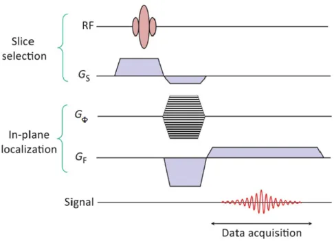
Firstly the slice selection take place applying the RF pulse simultasionely with the slice-selective gradient. After that, the phase encoding is on for a short amount of time and then it is turned off. Finally the frequency encoding is turn on during the readout of the signal (Figure 19).

Figure 19 NMR pulse sequence diagram. In a sequence diagram it is common to find a negative lobe to

correct the phase dispersion of transverse magnetization that occurs concomitant with application of the main Gz gradient (taken from [2]).

The signal is stored in a matrix known as k-space, trough the Fourier transform it the image in the real space is obtained.

33

2.1.1 Readout signal and k-space

The readout MR signal is the combination of plenty RF waves characterized by different amplitudes, frequencies and phases, containing spatial information. The spatial encoded raw data are arranged into an array of numbers representing spatial frequencies in the MR image. This is a matrix of frequencies (kx,ky), the so called k-space.

The k-space is commonly displayed like a rectangular grid where the axes, kx and ky, represent spatial frequencies respectively in the x and y directions rather than positions.

Each k-space point contains spatial frequency and phase information about every pixel in the final image. Conversely, each pixel in the image maps every point in k-space.

Figure 20 Representation of k-space. It is a grid of raw data of the form (kx,ky) obtained directly from the

MR signal.

The k-space grid is filled by frequency and phase encoded with magnetic gradient fields. During frequency encoding, gradient amplitude is constant and different data are acquired along kx at different times of echo sampling. During the phase

34

duration time is constant. Each ky line represent the point that are collected for a

given amplitude of the phase encoding gradient [5].

Data near the centre of k-space corresponds to low spatial frequencies, whereas data from the periphery relates to high-spatial frequencies, different parts of the k-space influence the apparence of MR images: line around the centre determine the contrast of image while the outer lines of the raw data matrix provide information on image spatial resolution.

The individual points (kx,ky) in k-space do not correspond one-to-one with

individual pixels (x, y) in the image, but they may be converted to one another using the FT. To go from a k-space data to an image a 2D inverse FT is required.

2.2 Image contrast

Depending on what it is necessary to visualize in an MR image, it is needed to enhance a type of contrast. The Proton Density (PD), the spin-lattice relaxation time (T1) and the spin-spin relaxation time (T2) are intrinsic properties of the

samples; in general, images have contrast that depends on one of these parameters. The contrast of MR image can be manipulated by varying several parameters among which the main ones the Repetition Time (TR) and the Echo

Time (TE).

 TR is the length of time between corresponding consecutive points on a repeating series of pulses and echoes. It determines how much longitudinal magnetization recovers between each pulse.

 TE refers to the time between the application of the radiofrequency excitation pulse and the peak of the signal induced in the coil. TE controls the amount of T2 relaxation.

The manipulation of these parameters permits to obtain images where contrast depends on the time constants T1 or T2 (that describe how long the magnetization

35

takes to get back to equilibrium after an RF pulse) or on proton density (it is related to the number of hydrogen atoms in a particular volume).

The TR dominates T1-weighted images, in these type of images, a short TE and a

short TR are required. The intensity of the image pixels is proportional to the protons concentration and it depends on the spin-lattice relaxation time of the sample. In presence of a long T1, the magnetization will take longer to recover

back to the equilibrium. This means that a short TR will make dark pixels compared to pixels associated with short T1, like fat, which appears brighter.

Bright pixels on T1 are associated with short T1 values. Water is characterized by

a long T1 giving a weak signal.

In T2-weighted images, water give the highest signal intensities, producing a

bright appearance, because of its long T2.

The intensity of the image pixels is proportional to the protons concentration and it depends on the spin-spin relaxation time of the sample.

The magnetization will take longer to decay and the signal will be grater, so it will appear brighter in the image than the signal from tissue with a short T2 (like fat).

In these type of images, a short TE and a short TR are required. These images are dominated by TE.

In PD weighted images high PDs give high signal intensities which in turn have bright pixels on the image. The signal contrast is derived from the density of spins in a given volume because the intensity of the image pixels is proportional to the protons concentration in a voxel. In these type of images, a short TE and a long TR are chosen to minimize both weightings.

To sum up (Figure 21), sequences with:

 Long TR and short TE return PD weighted images  Short TR and short TE return T1 weighted images

36

Figure 21 Contrast dependence on TR and TE

Maps

It is possible to obtain maps, in which each pixel contains information not about the intensity of the signal, but about relaxation time either T1 or T2. These maps

can be obtained by acquiring series of MR images with different levels of T1 or T2

weighting and performing nonlinear regression on the signal (see section 5.5). In conclusion, starting from an image the extrapolation of the relaxation times and the consequently interpretation of them is a great approach to interpreting MRI images and to attributing physiological meaning to them.

2.3 Sequences

The basic concept of MRI is the magnetic field inhomogeneity that induce spins precess at differing Larmor frequencies according to their location in the sample. All MR images are produced using pulse sequences [4]. The architecture of a sequence consists of radiofrequency pulses and gradient pulses which have carefully controlled durations and timings. There are many different types of sequences, but they all have the timing values TR and TE, which can be modified.

37

Spin echo (SE) pulse sequence is one of the earliest developed and still widely

used of all MRI pulse sequences, it is also known as a Hahn echo. The pulse sequence timing can be adjusted to give T1, PD or T2-weighted images. Dual echo

and multi-echo sequences can be used to obtain both PD and T2-weighted images

simultaneously.

From this point (x,y,z) notation it is referred to the rotating frame.

2.3.1 Spin echo

The SE sequence consists of a 90° applied on the x-axis pulse after which the spins dephase naturally for a certain time. Then a 180° pulse is applied on the y- axis causing the flips of all the spins of an angle of 180° [6].

Following the 90° pulse, spins in a region of relatively high magnetic field precess faster, while those in a region of relatively low magnetic field precess slower. After a certain time t, the phases of the spins across all these regions are sufficiently different to degrade the overall magnetization.

The application of the 180° pulse has the effect of reflecting the spins in the direction of the applied pulse. The spins continue to precess, but their relative motion is now precisely reversed. This means that the 180° pulse does not change the precessional frequencies of the spins, but it does reverse their phase angles. After a time equal to the delay between the 90° and the 180° pulse, those regions which were precessing faster and accumulated more phase difference undo their phase accumulation at a faster rate.

The result is that all the spins are back in phase and the total magnetization reaches a maximum, producing the echo.

The 180° RF pulse is applied at time TE/2, TE being the time between the center of the first RF pulse and the peak of the spin echo. The sequence is repeated at each time interval TR (Figure 22).

38

Figure 22 Spin echo diagram in the rotating frame (taken from Medical Radiation Resources).

The phase-reversal implies that the echo height will only depend on T2 and not on

the magnetic field inhomogeneities (no dependence from T2*) or on tissue

susceptibilities. The spin echo signal is given by:

𝑆𝑆𝐸 = 𝑆0𝑒𝑥 𝑝 (−

𝑇𝐸 𝑇2

) . (40)

2.3.2 Sequences based on the spin echo

The main sequences are based on the SE. A variation on the spin echo sequence is the so called inversion recovery (IR) which has an extra 180° RF before the 90° pulse. An IR pulse sequence is a spin echo pulse sequence preceded by a 180° RF pulse. This pre-pulse flips the longitudinal magnetization to its negative value. The time elapsed between the preparatory 180° pulse and the 90° readout pulse is termed time to inversion (TI) separated a timing parameter, specific of this sequence.

IR is often used to make signal ‘suppression’, since, tissues regain Mz at different

longitudinal relaxation rates determined by their T1 relaxation times. By selecting

39

90° readout pulse is applied at the exact time when longitudinal magnetization reaches the null point for the signal that is necessary to suppress. If a 90° excitation and two 180° refocusing pulses are used it is the so called

double spin-echo method [7].

Figure 23 Double spin echo pulse sequence (taken from [2]).

When after the 90° pulse an echo train by successive 180° is induced, a new sequence is obtained, the so called Carr–Purcell–Meiboom–Gill (CPMG).

The initial 90° pulse is on the x-axis and the train of 180° pulses is on the y-axis and all the echoes are positive. On the CMPG is based the sequence widely used in this work the Multi Slices Multi Echo (MSME).

40

Figure 24 Pulse sequence of MSME (taken from Bruker manual).

RARE (Rapid Acquisition with Refocused Echoes) sequence is based on

multiple-echo sequence filling more than one k-space trajectory in a single excitation this is the reason because of it is also named Fast Spin Echo (FSE) or Rapid Spin Echo (RSE).

Multiple spin echoes are generated using the CPMG sequence with slice selective RF pulses. Each echo is separately phase-encoded, and the phase encoding is incremented within one echo train to accelerate the acquisition. It is possible to obtain two or more echo-images with different effective TEs. The sequence scheme is the same of the MSME (Figure 24).

ZTE (Zero echo time) sequence is based on a non-selective excitation and a signal

acquisition in the presence of a constant gradient, a particular features is zero echo time. ZTE is a radial acquisition method, performing center-out readouts.

2.3.3 Gradient echo

In the gradient echo sequence, the angle used to flip the magnetization in the x-y plane is smaller than 90°. The sequence used in this work is the Fast Low Angle SHot (FLASH).

41

Figure 25 Pulse sequence of FLASH (taken from Bruker manual).

A negative gradient lobe is applied after the RF pulse causing a rapid dephasing of the transverse magnetization Mxy, faster than FID that is acquired in a spin-echo.

To rephasing spins, immediately after the negative lobe a positive gradient is applied. Spins that were precessing at a low frequency due to their position in the gradient will now precess at a higher frequency because the gradient will now add to the main field, and vice versa. After a certain time spins will all come back into phase along the y-axis forming the gradient echo.

A crucial point is that the positive gradient can compensates only the dephasing caused by the negative gradient lobe, it can’t refocus dephasing due to the main magnetic field inhomogeneities or spin-spin relaxation how happens in the spin echo sequences.

If S0 indicate the initial height of the FID, the height of the echo is thus determined by the FID decay curve which depends on T2*:

𝑆𝐺𝐸= 𝑆0𝑒𝑥 𝑝 (

𝑇𝐸

𝑇₂∗) . (41)

Remembering that T2* is a composite relaxation time which includes T2,

inhomogeneities due to the main field and tissue susceptibility, and diffusion of the protons (see section 1.4.1). In this case images acquired using a gradient echo are T2* weighted. Of course playing with the flip angle and the TR, it is possible

42

acquire gradient echo images T1 weighted or PD weighted for more details look at [2].

2.4 Single Voxel Spectroscopy

The single voxel spectroscopy (SVS) is one of the two method through which it is possible to perform the Magnetic Resonance Spectroscopy (MRS); the second method is the multi-voxel spectroscopy.

In the SVS the signal comes from a volume limited to a single voxel, the volume of interest (VOI) is selected and a spectrum obtained from it, whereas in the multi-voxel MRS spectra are obtained from multiple voxels in a single slice of sample.

In this work the MRI technique has been supplied by the SVS as it will be show in the chapters 5 and 6.

The two sequence most widely used in MRS are the PRESS (Point-RESolved Spectroscopy) and the STEAM (STimulated Echo Acquisition Mode). PRESS sequence results really useful for the purposes of this thesis, the acquisition is fairly fast (1 to 3 minutes) and the spectrum is easily obtained, it is the dominant method for ¹H spectroscopy used for single and multi-voxel studies. The sequence is based on the double spin-echo; the RF pulses have flip angles of 90°-180°-180° so the signal emitted by the voxel of interest is thus a spin echo. It works identically as in MR imaging but the signal is sampled without the read out gradient (see section 2.1: Frequency encoding) since the frequency differences are used to constitute the spectrum and not the position. The 90° pulse is followed by two 180° pulses so that the primary spin echo is refocused again by the third pulse. Each pulse has a slice-selective gradient on one of the three principle axes and the protons within the voxel are the only ones to experience all three RF pulses.

So using a combination of magnetic field gradients and frequency-selective 180° pulses, a three-dimensional voxel of well-defined position and size is selected and its spectrum is then collected and analyzed.

43

Figure 26 Selection of a cube with a PRESS sequence. The three RF pulses within the sequence are marked

and the selected regions after each pulse are shown for an cubic object [7].

All the sequences described in this section have been used for the aim of this work. These and many others are implemented in the software package of the Bruker spectrometer used for the experiments. This latest generation instrument make available various acquisition and processing tools and broad spectrum of applications. The experimental setup used to perform the analysis will be describe deeply in the next chapter.

44

3. Experimental Setup

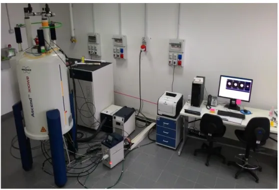
MRI technique has been performed with a Bruker NMR Spectrometer 300 MHz/89 mm ASCENDTM _{. The spectrometer consists of the following subunits:}

• Operator console including the host computer, monitor and the keyboard • Console containing the electronic hardware

• Magnet system including the shim system and the probe.

45

Magnet

The main component of the MR system is the magnet, which generates the magnetic field required to induce NMR transitions.

The Bruker Ascend magnet design features advanced superconductor technology, enabling the design of smaller magnet coils, thus resulting in a significant reduction in physical size and magnetic stray fields [Bruker User Guide].

The Exclusion Zone (the area inside the magnet's 5 Gauss field line) is completely confined inside the instrument, as shown below in Figure 28.

Figure 28 Fringe field plot (taken from Bruker manual).

At MNR Laboratory of Physics Department of Salerno, the spectrometer is equipped with a superconducting magnet that generates a field of 7 Tesla (300 MHz). As known, superconducting magnets at temperatures approaching absolute zero, 0K, have zero electrical resistance. A superconducting wire held below its transition temperature will give the possibility to get a continuously circulating

46

current. To maintain a superconducting system the magnet core is cooled to very low temperature using nitrogen and helium. The spectrometer in our lab requires helium every 6 months and nitrogen every 15 days.

The magnet core consists of a large coil of carrying wire in the shape of a solenoid. At the center of the coil, the static field is very intense, to allow the analysis of the sample placed inside the field.

The superconductive magnet consists of several sections. Like a “thermos” the outer casing of the magnet is evacuated and inner surfaces are silvered. Next comes a bath of nitrogen which reduces the temperature to 77.35 K (195.8°C) and finally a tank of helium in which the superconducting coil is immersed in.

This tank is thermally isolated against the nitrogen bath by a second evacuated section as shown in the picture below [Bruker User Guide].

47

1 Bore insertion 6 Helium Tower

2 Bore 7 Metal Plug

3 Nitrogen Tower 8 Sample insertion

4 Nitrogen Ports 9 Vacuum

5 Helium Ports 10 Magnet

The helium and nitrogen tanks are wrapped around the magnet bore (central column). A metal plug normally closes off the top of the bore. Samples to be analyzed are introduced into the magnet via the top of the bore. Probes, which hold the sample and carry signals to and from the samples are inserted from the bottom, like in the micro-imaging case.

3.1 Probes

The spectrometer is equipped with a MicWB40 Probe in combination with the Micro2.5 Gradient System. The MicWB40 probe has been developed for micro-imaging of small objects (max. diam. 30 mm) in wide bore magnets (89 mm ID). The probe has an outer diameter of 40 mm and fits into the separate Micro2.5 gradient system.

Probe tuning and matching

The sensitivity of any probe will vary with the frequency of the signal transmitted to it and there exists a frequency at which the probe is most sensitive. Furthermore, this frequency may be adjusted over a certain range using capacitors built into the probe circuitry. Tuning involves adjusting the probe circuitry so that the frequency at which it is most sensitive is the relevant transmission frequency. Each coil in the probe will be tuned (and matched) separately. If the probe has been changed or the transmission frequency altered significantly, it may be necessary to retune the probe.

48

Whenever a probe is tuned it should also be matched. Matching involves ensuring that the maximum amount of the power arriving at the probe base is transmitted up to the coil which lies towards the top of the probe. This ensures that the minimum amount of the power arriving at the probe base is reflected back towards the amplifiers (and consequently wasted). It is also possible using an automatic tool ATM (Automated Tuning Routine) [Bruker User Guide].

Four different probes can be interfaced with the spectrometer:

1. Double Resonance Broadband Probe (BBI) – Liquid state

2. Probe Cross Polarization Magic Angle Spinning (CPMAS) - Solid state 3. Probe High Resolution Magic Angle Spinning (HRMAS)

4. Micro-Imaging Probe for Wide Bore Magnets

The latter is the one which has been used in this work (Figure 30, Figure 31).

Figure 30 Exchangeable coil insert.

49

3.2 Gradients

Usually, three sets of gradient coils are used in all MR systems: the x, y and z gradients. The gradient fields are produced by three sets of gradient coils one for each direction, can be applied in any direction or orientation. Each coil set is driven by an independent power amplifier and creates a gradient field whose z-component varies linearly along the x, y, and z-directions, respectively.

These fields are normally applied only for a short time as pulses through large electrical currents applied repeatedly in a carefully controlled pulse sequence. During an image acquisition, when the current is pulsed through the gradient coils in the presence of the static magnetic field, the gradient pulse produce Lorentz force which causes vibrations of the coils against their supports. The characteristic ‘knocking’ noise heard when an images is acquired is due to this reason.

The three sets of gradient coils are included in the MR system: Gx, Gy and Gz

create a linear variation in the longitudinal magnetic field strength as a function of spatial position as seen in the section regarding the spatial encoding (section 2.1).

3.3 Nmr software

TopSpin and ParaVison are two processing software provided by Bruker.

TopSpin is used for NMR data analysis, acquisition and processing every time a spectrum is acquired.

TopSpin is designed with a highly intuitive interface and provides easy access to vast experiment libraries including standard Bruker pulse sequences and user generated experiment libraries. [https://www.bruker.com/products/mr/nmr/nmr-software/nmr-software/topspin/overview.html].

To perform MRI data acquisition and reconstruction has been designed a software package called ParaVision. It can be used to analyse, visualize and manage the data generated on Bruker systems.

50

A sub-package of ParaVision program is the Image Sequence Analysis (ISA) Tool, which provides a general and flexible framework for the visualization and statistical analysis of such sequences of images. It has been used as explained in the chapter 5 and 6.

The Bruker NMR Spectrometer is only one of the wide range of product available as research tool; NMR and MRI technology is continuously developing. Much of the success of these techniques is due to its flexibility and its potential for probing the properties of complex materials.

The use of NMR and MRI has spread from medical area to a large range of application: quality control in industrial, research in building materials, wood, paper and cultural heritage, geohydrology, plant physiology, well logging, cosmetic [8][9], paper industry [10], and food processing.

51

4. MRI Application

MRI born as a “safe” diagnostic protocol to obtain good resolution images of the patient and has gained in the last few years growing interest relying also on the absence of ionizing radiation.

Nowadays is the most dominant imaging method employed in medical investigation. It provides the best soft-tissue contrast among the existing imaging modalities.

The development of superconductive magnets to generate stronger magnetic fields and the new computing technologies have contributed to make MRI ever more performing.

4.1 Medicine

MRI plays an increasingly important role in clinical diagnosis; it helps to visualize the structures of the body that include water and fat molecules. MRI is a technique for taking very clear and detailed pictures of tissues and internal organs. Using different acquisition parameters (TE,TR), MRI allows acquiring high quality images with the possibility to enhance different types of tissues. Because of its high soft-tissue contrast and multiplanar imaging capability, MRI can reach excellent anatomic details. It is more sensitive than computed tomography (CT)

52

and allows differentiation among fat, muscle, tendon, bone and vascular structures based on characteristic signals. Due to these reasons, MRI has a major role in the evaluation of soft tissue tumours, for recognition, staging, and treatment planning of soft tissue and bone tumours [11]. This type of imaging allows also the detection of recurrent tumours in the presence of non-ferromagnetic metallic implants [12].

The appealing properties of imaging by magnetic resonance bring to several application like integration of MRI with PET (Positron Emission Tomography) or in conjunction with radiation therapy treatment.

In medical research, a current and increasingly in development application of high field MRI is the study of the brain. MRI currently is the most versatile and informative imaging modality for the central nervous system (CNS) [13], the investigation of the CNS from microstructure to physiology of the brain is under continuous investigation [14]. Several pathologies, like multiple sclerosis, brain tumours, aging-related changes and cerebrovascular diseases can be studied with high field (7-11 T) technologies [15][16].

One of the latest neuroimaging technique is the functional Magnetic Resonance

Imaging (fMRI), used to visualize functional activity in the brain, investigate

human brain function and cognition, measuring changes in blood flow in different parts of the brain comparing healthy and abnormal brain states. fMRI can detect small changes in the signals, associated with neuronal activity in the brain, which are used to produce magnetic resonance images. The haemoglobin contained in the blood exhibit different properties depending on whether or not it is bound to oxygen. When a specific activity is performed in the area of the brain responsible for that activity, the blood flow increases. This phenomenon is the so called Blood

Oxygen Level Dependent (BOLD) effect. Setting specific parameters MRI can

detect this increasing and BOLD can be used to create maps of brain activity. It is used to observe brain structures and to determine which parts of the brain are handling critical functions. One of the specific applications of fMRI is for example the investigations of abnormal functioning in psychological disorders.

53

fMRI may also be used to evaluate damage from a head injury or Alzheimer's disease.

It is also possible to combine fMRI with complementary imaging modalities, one of these is the use of the Diffusion Tensor Imaging (DTI).

Whereas with the fMRI it is possible to collect information about the synchronization of brain activation across different brain areas during rest or during a specific activity, DTI examines the diffusion of water in the brain to infer the integrity of white matter fibers. This technique allows to measures how water molecules diffuse through brain areas. A disease like stroke or tumor reduce this diffusion, so DTI allows to locate the anomalies. Using diffusion gradients the water diffusion in the brain is examined in several directions. The use of MRI in neuroscience research and in clinical neurological applications is more and more rapidly expanding [17].

4.2 Porous media

It easy to find a wide range of specific application of the NMR technique and of the imaging by magnetic resonace related to the study of porous media [18] [19]. Through the knowledge of the water distribution inside the porous structure, it is possible to identify the degradation processes and understand how to manage it. Relying on the ability of MRI technique to achieve very high resolution images its use has found an interesting application also in the field of the study and preservation of artifacts related to our cultural heritage [20][21][22][23].

MRI results to be a good procedure to investigate the porosity of different lapideous materials (i.e.: marble, granite) as well as monuments or walls of historical buildings. Injecting a water agent contrast liquid in a porous material, the mobile molecules are confined in the matrix of the stones filling the pores. NMR signal shows an intensity that gives quantitative measurements of the content of the liquid.

An example is the study on the damage due to salt coming from seawater and from the environment. Salt crystallisation of porous media is widely recognized as