Indirect microfabrication of biomimetic materials for locomotor tissues regeneration

(1)

University of Pisa

Faculty of Engineering

PhD Course in

Chemical and Material Engineering

XXIV Cycle SSD Ing-Ind 34

PhD Thesis

Indirect microfabrication

of biomimetic materials for

locomotor tissues regeneration

Carmelo De Maria

(2)

(3)

University of Pisa

Faculty of Engineering

PhD Course in

Chemical and Material Engineering

XXIV Cycle SSD Ing-Ind 34

PhD Thesis

Indirect microfabrication

of biomimetic materials for

locomotor tissues regeneration

Tutor PhD student

Ing. Giovanni Vozzi Carmelo De Maria

Prof. Giuliano Cerulli

(4)

(5)

Abstract

Tissue Engineering is a new field of the scientific research with a fi-nal aim to develop techniques for regeneration, repair, maintenance and growth of tissues or organs to overcome the limitations intrin-sic to current therapeutic strategies. A fundamental element of this approach is the scaffold. The scaffold is a 2D and 3D structure, made with natural or synthetic material, that emulates the extra-cellular matrix, that is it offers mechanical, topological, biochemical and chemical stimuli to promote cellular organization, growth and differentiation to create a tissue with adequate functional and mor-phological characteristic. Scaffolds are therefore characterized by peculiar features (e.g. porosity, mechanical properties) determined by the material and by the manufacture process. Nowadays, the ad-ditive Rapid Prototyping (RP) techniques are the best approach to realize complex structures, because overcome all the problem of con-ventional (subtractive) techniques. Despite the high potential, RP techniques are not always compatible with all materials. In particu-lar, hydrogels, an elective class of biomaterial for scaffolds realization because the lot of features in common with the extracellular matrix, results very difficult to be processed. To overcome these limitations and take advantage of all benefits of rapid prototyping, indirect rapid prototyping (iRP) was developed, that is the realization of scaffold or

(6)

iRP offers the benefits to fabricate composite scaffold realized with different materials, with less waste and high fidelity in the realiza-tion of the designed structure. One of the critical aspect of this class of realization process is the extraction of the final object from the mold. A possible solution, proposed in this research, is to realize the mold with low melting point materials, dissolving the mold at the end of the process without damaging the scaffold. Moving in this direction, the attention of this research is focused on two classes of materials, low melting point waxes and agarose. Two alternative RP techniques have been evaluated: new modules of the PAM2 _{, a}

con-tinuous flow system, and a inkjet-based device have been designed and realized to test the feasibility of this approach. In addiction, an alternative approach to fabricate agarose microstructure, by ex-ploiting the different agarose gelling ability in DMSO and water, has been proposed. In a future perspective, casting of the desired ma-terial, which may include also cells, should be performed directly in the surgery room using an anatomical shaped mold designed on the patient needs. Following this approach, two plugins for bioimages de-noising and segmentation, based on the ITK library, have been implemented for the OsiriX software. To further test the versatility of the two microfabrication devices, other applications have been ex-plored, such as the realization of microfluidic circuits using PAM2_or

(7)

(8)

(9)

Done is better than perfect. Mark Zuckerberg

(10)

(11)

Acknowledgements

E’ la prima volta che mi trovo a scrivere i “famosi” ringraziamenti e, sincero, non so proprio come iniziare. Non so neanche se scrivere in italiano o in inglese ... Bah, iniziamo in italiano, magari strada facendo si cambia.

Un enorme grazie a Giovanni: Gio’, facendo due conti sono sei anni! Era il 13 marzo del 2006 (e chi se lo scorda!) quando abbiamo com-pilato i documenti per la tesi triennale!

Grazie al Prof. Cerulli che ha creduto e crede nel valore della ricerca, supportando, attraverso la Nicola’s Foundation, questo lavoro di dot-torato.

Un grazie speciale alla Prof. Arti: se son “salito” al Centro Piaggio `

e perch´e c’era lei.

I would like to thank also Professor Thomas Boland for sharing with me a lot interesting ideas and good coﬀees! I take this opportunity also to thank all the guys of the lab at UTEP: Maria, Sylvia, Julio I hope to see you again!

Un grazie enorme a Daniele “l’elbano”, che ha praticamente salvato il mio dottorato con una gita sul lago di Garda. Un grazie a tutti i ragazzi “bio” del centro: Federico e il Domenici (si lo so che siete CNR), Annalisa, Tommaso, Gianni, Giorgio, Serena, Nicole, Yudan,

(12)

becchiamo come Sandra e Raimondo. E come non ringraziare la mia “pupilla” Aurora ed il mio “angelo custode” Rodrigo, gli ultimi sei mesi al centro Piaggio sono stati fantastici. E poi un mille grazie al mio compagno di tante domeniche, Manuel, al mio salvatore ed alter ego, Fabio, a tutti i ragazzi di robotica, Konan Manolo, Giorgio, Alessandro, Felipe, Matteo, Spillo, Andrea. E Fabio, e le giornate a ragionare su come costruire quella benedetta stampante, con io che mi presentavo con disegni fatti a mano e lui, con santa pazienza, ad ascoltarmi. E poi Agnese, Andrea, Laura, Francesca...

Sto scrivendo queste due righe mentre sono lontano da Pisa: caspita sono passati pi`u di otto anni da quando sono arrivato sotto la torre... Come non ricordare la mitica casa di via Risorgimento con i miei (purtroppo) ex-coinquilini Roberto, Gigi, Peppe, e le mie quasi coin-quiline! A proposito di di amici e coinquilini, un grazie enorme a

Koke, Pedro, Ivan: Hola, ¿qu´e pasa? Afterparty? E poi i

com-pagni degli ultimi due mesi trascorsi a scrivere la tesi, “Dio Mio, dovetelametto” Peppe, “dul¸cao-arpeggio-volluto-indriya” Lorenzo e “Dexter” Riccardo.

Penso di non averlo forse mai detto, sicuramente non l’ho mai scritto, ma ho sempre pensato di avere una famiglia meravigliosa: grazie mamma, grazie pap`a, grazie Anto’ ! Vorrei dire grazie anche a nonna, io ci provo, magari mi sente...

Dulcis in fundo, un bacio a Chiara che ha sopportato i miei cambi-amenti d’umore: non volevo scrivere quest’ultima parte, pare porti sﬁga, incrociamo le dita...

(13)

List of Figures

1 Rapid Prototyping process . . . 7

1.1 Edge preserving plugin organization . . . 16

1.2 Edge preserving plugin panel . . . 17

1.3 Edge preserving ﬁlter performance analysis . . . 18

1.4 Sigmoid ﬁlter transform function . . . 22

1.5 Level Set plugin organization . . . 24

1.6 Level Set plugin ﬁlter panel . . . 25

1.7 EPﬁlter and LSSegmentation plugins . . . 26

2.1 PAM2 _{system . . . .} ₂₉

2.2 PAM2 power supply . . . 30

2.3 TCS module . . . 31

2.4 TDP module . . . 32

2.5 pCam device and software . . . 33

2.6 pCam scheme . . . 35

2.7 Drop formation . . . 38

2.8 Drop diameter . . . 40

2.9 Thickness of solidiﬁed layer . . . 42

(18)

2.11 Wax volumetric shrinking . . . 45

2.12 Wax deposition process . . . 45

2.13 PAM2 _{printing paths . . . .} ₄₆

2.14 Wax line-width characterization . . . 46

2.15 Examples of wax structures . . . 47

2.16 Defect analysis of wax patterns . . . 48

2.17 Filler eﬀects on 3D wax structures . . . 50

2.18 Three dimensional wax structures . . . 50

2.19 Agarose line with PAM2_{system . . . .} ₅₂

2.20 Agarose line-width as function of PAM2 _{working parameters . . .} ₅₃

2.21 Agarose line-width as function of PAM2 working parameters . . . 54

2.22 Agarose microfabrication . . . 54

3.1 Penelope - First prototype . . . 58

3.2 Penelope - Deposition plane . . . 59

3.3 Penelope - Temperature controlled cartridge . . . 60

3.4 Penelope - Second prototype . . . 61

3.5 Penelope - Second prototype improvements . . . 62

3.6 Penelope - Control software . . . 62

3.7 Penelope - Control software architecture . . . 63

3.8 Penelope - Calibration image . . . 67

3.9 Penelope - Horizontal resolution . . . 68

3.10 Penelope - Vertical resolution . . . 69

3.11 Printed agarose structures . . . 69

3.12 FEM geometry of water diﬀusion . . . 71

3.13 FEM results of water diﬀusion . . . 73

(19)

LIST OF FIGURES

3.15 Mechanical behavior of printed structures . . . 76

3.16 Printed agarose line . . . 77

3.17 FEM of drop impact - boundary conditions . . . 81

3.18 FEM of drop impact - Model results . . . 83

3.19 FEM of drop impact - Drop shape . . . 83

3.20 Viability results . . . 86

4.1 Mold design . . . 89

4.2 2D wax mold with ﬁnal part . . . 90

4.3 3D wax mold with ﬁnal part . . . 90

4.4 PDMS microﬂuidic circuits . . . 93

4.5 Gel microﬂuidic circuits . . . 93

4.6 Agarose printing . . . 96

4.7 Gelatin printing . . . 96

4.8 CNTs printing using Penelope . . . 99

(20)

(21)

List of Tables

1 Examples of indirect rapid prototyping . . . 6

2.1 Wax applications in TE . . . 36

2.2 Filler results . . . 49

3.1 Agarose gelation time . . . 68

3.2 FEM of diﬀusion process - Model parameters . . . 72

3.3 FEM of drop impact - Model parameters . . . 82

4.1 Microﬂuidic circuit accuracy . . . 94

(22)

(23)

List of Acronyms

CAD Computer Aided Design

CAM Computer Aided Manufacturing CAx Computer Aided x

CNT Carbon Nanotube

DEA Dielectric Elastomer Actuator DMSO Dimethyl sulfoxide

DOD Drop On Demand dpi Dot per inch

ECM Extra-Cellular Matrix FEM Finite Element Modeling GUI Graphical User Interface HA Hydroxyapatite

(24)

ITK Insight ToolKit

MVC Model-View-Controller PAM Pressure Aided Microsyringe PAM2 Piston Aided Microsyringe

PAM2 PAM modular micro-fabrication system

pCam PAM2 camera

PDMS Polydimethylsiloxane ROI Region Of Interest RP Rapid Prototyping SNR Signal-to-Noise ratio

SWNT Single Walled carbon NanoTube TE Tissue Engineering

(25)

Introduction

Tissue Engineering (TE) is an interdisciplinary field in which knowledges from physics, chemistry, biological sciences and engineering are combined to design, built, modify, growing up and maintenance living tissues (1), with the aim to overcome the intrinsic limits of traditional approaches based on transplants (lack of donors (2) and histocompatibility problems(3)) and of artificial prothesis (in-flammatory response (4) and complexity of biologic systems (5)).

In the scaffold based TE (6, 7), the construction of a bioartificial tissue be-gins with a in-vitro formation, in an environment which provides mechanical and metabolic support, of a tissue construct starting from cells seeded onto a scaffold. The scaffold usually is porous a structure realized in a suitable geom-etry (8) using a degradable biomaterial, often modified to be adhesive for cells or selective for a specific cell type. The scaffold provides mechanical stability to the tissue construct in the short term and gives a support for the three dimen-sional organisation of cells until the tissue completion; as the tissue grows up the material is degraded by hosted cells with a rate similar to the biosynthesis rate of extracellular matrix (ECM). In a second phase, this construct is implanted in the appropriate anatomic site, where there is the in-vivo remodeling for the construction of functional architecture of the tissue or the organ. Some steps can be omitted: for example, to engineer cardiac valves or blood vessels,

(26)

de-cellularized tissues have been used as scaﬀold to attract endogenous cells (9). The realization of 3D tissue substitutes requires also a biological model, i.e. an appropriate source of proliferating not-immunogenic cells, with appropriate bi-ological functions, a protocol for cells expansion which not alters the speciﬁc phenotype, and cell culture techniques which allow to reach high cell densities (> 106_cells/cm3_{). Stem cells could be a solution, but several problems are still}

unsolved (10, 11).

The main challenge of 3D cultures is the accomplishment of a controllable and homogeneous cell behavior within the entire 3D volume. The cell behav-ior is characterized by both an intrinsic variability related with the properties of the cell itself and an extrinsic variability related to the microenvironmental properties. These two sources of variability can both induce heterogeneity of cell fate within the 3D domain, leading to an undesired nonhomogeneous 3D culture structure. The intrinsic variability depends only on the cell source and cannot be controlled during the culture, whereas the extrinsic variability can be minimized by strictly controlling the microenvironmental properties that depend on the experimental setup used for culturing cells. Inside a bioreactor, a “liv-ing organism” simulator, temperature, pH, O2 and metabolites concentration,

waste removal, mechanical loading (12, 13, 14) can be controlled. Biochemi-cal (15, 16, 17), mechaniBiochemi-cal (e.g. stiffness) (18, 19, 20), topologiBiochemi-cal (e.g. pore size) (21, 22, 23, 24) stimuli can be transmitted by the scaffold to correctly engineering a tissue, maintaining a complete functionality. Biocompatibility, bio-degradability and bio-absorbability with a controlled degradation rate bal-anced with cell growth in-vitro and/or in-vivo (25, 26), sterilizability (27) and reproducibility (28) are other fundamental properties of scaffolds.

Research on design and realization of 3D scaﬀold is directed on polymeric materials and bioceramics. Biological (natural) polymers are usually ECM

(27)

com-ponents, as collagen, elastin, hyarulonic acid or can be polysaccharides with vegetal origin, as alginate and agarose (29, 30). The ECM itself was used with some success as scaffold material (31). The main advantage of biological poly-mers is that they mimic ECM and so are an ideal environment for cell growth, ensuring also atoxicity and cellular adhesion. The drawback is that they are less resistant both from mechanical and chemical point of view, are less stable and more expensive. Most of the natural polymers can be formed into hydro-gels, colloids formed by long polymeric chains with high water content (up to 99%), representing an ideal class of material to realize bioinspired scaffold for the strong analogies with ECM (26). Synthetic (man-made) polymers are more flex-ible, more predictable and more processable into different size and shape respect to natural origin polymers. Their physical and chemical properties can be easily modified and the mechanical and degradation characteristics can be altered by their chemical composition of the macromolecules: functional groups and side chains can be linked to peptides or other bioactive molecules (26). The most ex-tensively used synthetic polymers are poly-glicolic acid (PGA), poly-lactic acid (PLA) and their copolymers, polycaprolactone (PCL) and polyethylene glycol (PEG). Hydrogels from synthetic polymers, mainly based on PEG-based poly-mers, result less suitable for scaffold realization respect the natural counterpart, because the citotoxicity of the crosslinking agents. Bioceramic materials, mainly used in bone-tissue engineering applications, includes hydroxyapatite, the inor-ganic component of bone, three calcium phosphate, bioglasses and glass ceramics (24). In general, ceramic biomaterials are able to form bone apatite-like material or carbonate hydroxyapatite on their surface, enhancing their osteointegration. Brittleness and slow degradation rates are disadvantages associated with their use. Examples of combination of natural and synthetic polymers together with

(28)

bioceramic materials are numerous with the aim to integrate the best features of each components (32, 33, 34).

Porosity, biocompatibility and biodegradability, together with other final properties of the scaffold, often, are induced by manufacturing techniques. To realize three dimensional scaffolds can be used several techniques, from more conventional, such as textile techniques, molding processes, until the more re-cent microfabrication techniques which use a Rapid Prototyping approach.

The term Rapid Prototyping (RP) indicates a group of technologies that allows the automatic realization of physical model based on design data using a computer. Rapid prototyping processes belong to the generative1 _(or

addi-tive) production processes. In contrast to abrasive (or subtracaddi-tive) processes such as lathing, milling, drilling, grinding, eroding, and so forth in which the form is shaped by removing material, in rapid prototyping the component is formed by joining volume elements. This approach applied to tissue engineering takes the name of bioprinting (35), deﬁned as the use of computer-aided trans-fer processes for patterning and assembling living and non-living materials with prescribed 2D or 3D organization in order to produce bio-engineered structures serving in regenerative medicine, pharmacokinetic and basic cell biology stud-ies. Bioprinting can be inserted in the broader ﬁeld of Computer Aided Tissue Engineering (CATE), the application of advanced computer-aided technologies to tissue engineering problems (36).

In general, RP techniques follow a CAD/CAM approach (Computer Aided Design/Computer Aided Manufacturing). Practically, the design of the object is done using a computer (CAD) which then sends to the machine the instructions

1_{Generative production processes is the generic (seldom used in practice) to indicate a}

additive production process. More common are the expression solid freeform manufacturing (SFM), or solid freeform fabrication (SFF) which emphasizes the ability to produce framed solids by means of free form surfaces.

(29)

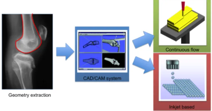
to obtain the desired shape (CAM), fabricated layer by layer. In some cases (especially in biomedical field) the geometry is extrapolated by dedicated seg-mentation algorithms (see sec. 1.3), from CT scan or RM scan. To proceed with the production of a rapid prototyping model it is first necessary to establish the auxiliary geometries (supports, walls, etc) (if) required for the construction and to establish the machine parameters. Finally, all data, the geometry and the supports, are together sliced into layers by mathematical means providing the layer information that, together with machine specific parameters, is necessary for the production of each layer (37). The two-dimensional layer is shaped (con-toured) in an (x-y) plane. The third dimension results from single layers being stacked up on top of each other, but not as a continuous z-coordinate. So, in the strict sense, rapid prototyping processes are therefore 21_/₂_{D processes, that}

is stacked up 2D contours with a constant thickness. Joining the layers in the z-direction with one other is achieved in the same way as joining them in the x-y direction. The energy or the amount of binder necessary for the joining on (it depends on the tecnology used) is proportioned in such a way that not only the layer itself but also part of the preceding layer is aﬀected and thus joined to the new layer. For the implementation of the rapid prototyping principle several fundamentally diﬀerent physical processes are suitable:

• Solidiﬁcation of liquid materials (e.g photo-polymerization process (38)); • Generation from the solid phase:

– incipiently or completely melted solid materials, powder, or powder

mixtures (extrusion (28), ballistic (39) and sinter processes (34));

– conglutination of granules or powders by additional binders (3D printer

(30)

• Precipitation from the gaseous phase (e.g. Laser Chemical Vapor

Deposi-tion (41)).

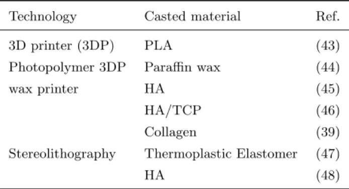
Other classifications have been also proposed (42). An important parameter to choose between different rapid prototyping techniques is the used material, in particular the chemical-physical properties which interact with the working methods of manufacture process. Most of fabrication techniques described above requires particular conditions (of pressure or temperature) which limits the ma-terial choice to realize 3D structure to synthetic polymers; a natural polymer as collagen, which has a low degradation temperature (40◦C), cannot be processed. As alternative, scaffold realization using natural biomaterial can be obtained by indirect fabrication techniques, starting from sacrificial mold realized by RP processes. This techniques, known as indirect Rapid Prototyping (iRP) or in-direct Solid Freeform fabrication (iSFF) (42) seems to be the most promising indirect fabrication technique, which allows in any case a satisfactory control on the external and internal scaffold architecture (tab. 1).

Technology Casted material Ref.

3D printer (3DP) PLA (43)

Photopolymer 3DP Paraﬃn wax (44)

wax printer HA (45)

HA/TCP (46)

Collagen (39)

Stereolithography Thermoplastic Elastomer (47)

HA (48)

Table 1: Examples of indirect rapid prototyping

So, overcoming the limits and taking the advantages of RP, the iRP process allows:

(31)

• realization of composite scaﬀolds, that are scaﬀolds realised with a wide

range of (bio-)material that are incompatible with other fabrication tech-niques;

• less waste of row material;

• high ﬁdelity in the scaﬀold realization respect to other RP techniques.

Figure 1: Rapid Prototyping process - Flow work of a RP process, from

image segmentation to realization.

One of the critical aspect of this approach is the extraction of the scaffold from the mold. Mechanical extraction may result in a damage due to scaffold fragile structure. Another solution is to melt the mold in a solvent (usually organic) and to wash the scaffold to eliminate traces of solvent and of the mold. This approach brings with itself a potential toxicity, and does not allow an immediate extraction of the piece from the mold (melting times are around twelve hours). A possible solution is to realize the mold with low melting point materials, dissolving the mold at the end of the process without damaging the scaffold. Moving in this direction, the attention of this research is focused on two class of materials, low melting point waxes and agarose, and on two microfabrication techniques: new

(32)

modules of the PAM2_{system, and a inkjet-based device have been designed and}

realized to test the feasibility of this approach. In particular, an alternative approach to fabricate agarose microstructure, by exploiting the diﬀerent agarose gelling ability in DMSO and water, have been proposed. In a future perspective, casting of the desired material, which may include also cells, should be performed directly in the surgery room using an anatomical shaped mold designed on the patient needs extrapolated from tomographic data (e.g. CT and MR scan). Following this approach, two plugins for bioimages de-noising and segmentation, based on the ITK library, have been implemented for the OsiriX software. To further test the versatility of the two microfabrication devices, other applications have been explored, such as the realization of microﬂuidic circuits using PAM2

or printing carbon nanotubes suspension for polymeric actuators.

This research project will be deeply described in the various chapter of this book, using ﬁg. 1 as guide. The ﬁrst chapter will describe the procedure to ex-tract geometrical information from bioimages, analyzing in detail two purposely

developed plugins. The second chapter is dedicated to PAM2 _{system, and to}

the micro-processing of paraﬃn wax. The inkjet based device, called Penelope, and the fabrication of agarose microstructures are treated in the third chapter, where the design of the system and mathematical modelling of fabrication pro-cess are described. The analysis of drop impact, to evaluate stress acting on ink-containing-cell, concludes this chapter. The fourth and last chapter gives an overview on possible applications investigated in this work using PAM2_and

(33)

Chapter 1

Image Analysis

Computer-Aided Tissue Engineering (CATE) enables the application of advanced computer-aided technologies and engineering principles to derive systematic so-lutions for complex tissue engineering problems (36). One of the bases of this new field is the representation and modeling of tissues and organs and their 3D reconstruction through design and fabrication of biological tissue systems and scaffolds at different hierarchical levels using a CAD/CAM approach. Virtual reconstruction of an anatomical parts starting from tomographic data is the topic of this chapter, which describes two plugins purposely developed in this research to de-noise and segment bioimages using OsiriX, an opensource image processing software dedicated to DICOM images.

1.1 ITK and OsiriX

In the Rapid Prototyping approach, the realization of custom made scaﬀolds, based on the patient speciﬁc needs and anthropometric data, begins with the virtual reconstruction of the anatomical part to be fabricated. For the extraction

(34)

of topological information from medical images, during this research two OsiriX plugins, based on the ITK library, have been developed.

1.1.1 ITK

The Insight Toolkit (ITK) is an open-source software toolkit (49, 50) for per-forming registration1_{and segmentation}2_{. ITK is implemented in C++, following}

the generic programming approach, so that the same code can be applied

gener-ically to any class or type that supports the operation used; it is so possible to

write software in terms of one or more unknown types T. At compile-time, the compiler makes sure that the templated types T are compatible with the istanti-ated code and the types are supported by the necessary methods and operators. Another important features in ITK is the memory management, which is imple-mented through reference counting, that is a count of the number of references to each instance is kept. When the reference goes to zero, the object destroys itself. In garbage collection, another popular approach in memory management, a background process sweeps the system identifying instances no longer refer-enced in the system and deletes them: the actual point in time at which memory is deleted is variable and this is unacceptable when an object size may be very large (think of a large 3D volume gigabytes in size). Reference counting instead deletes memory immediately (once all references to an object disappear). The ITK subsystems used in the developed plugins are listed below:

Data processing pipeline. The data representation classes (known as data

objects) are operated on by filters that in turn may be organized into data

1_{Registration is the task of aligning or developing correspondences between data.} _For

example, in the medical environment, a CT scan may be aligned with a MRI scan in order to combine the information contained in both.

2_{Segmentation is the process of identifying and classifying data found in a digitally sampled}

(35)

1.1 ITK and OsiriX

ﬂow pipelines. These pipelines maintain state and therefore execute only when necessary;

Level Set Framework. The level set framework is a set of classes for creating

filters to solve partial differential equations on images using an iterative, finite difference solvers including a sparse level set solver, a generic level set segmentation filter.

1.1.2 OsiriX

OsiriX (51) is an image processing software dedicated to DICOM images1 pro-duced by imaging equipment (MRI, CT, PET, PET-CT, SPECT-CT, Ultra-sounds, ...). It is fully compliant with the DICOM standard for image com-munication and image file formats. OsiriX has been specifically designed for navigation and visualization of multimodality and multidimensional images pro-viding 2D, 3D, 4D (3D series with temporal dimension) and 5D Viewer (3D series with temporal and functional dimensions). The 3D Viewer offers several ren-dering modes: Multiplanar reconstruction (MPR), Surface Renren-dering, Volume Rendering and Maximum Intensity Projection (MIP). All these modes support 4D data and are able to produce image fusion between two different series (e.g. PET-CT). OsiriX is so at the same time a DICOM PACS (picture archiving and communication system (52)) workstation for imaging and an image processing software for medical research (radiology and nuclear imaging). It results easy-to-use by clinician in the perspective of an active collaboration for the scaffold design. OsiriX supports a complete plugins architecture that allows to expand

1_{The Digital Imaging and Communication in Medicine (DICOM) Standard allows}

inter-operatibility of medical imaging equipment by specifying a set of media storage services, a file format, and a medical directory structure to facilitate access to the images and related information stored on interchange media.

(36)

the capabilities of OsiriX, using Cocoa framework (Objective-C language), and the ITK library, already embedded into the software.

1.2 Edge Preserving Smoothing Plugin

Real image data has level of uncertainty that is manifested in the variability of measures assigned to pixels. This uncertainty is usually interpreted as noise and considered an undesirable component of the image data. Blurring is the tradi-tional approach for removing noise from images. It is usually implemented in the form of convolution with a kernel. The effect of blurring on the image spec-trum is to attenuate high spatial frequencies. The drawback of image denoising (smoothing) is that it tends to blur away the sharp boundaries in the image that help to distinguish between the larger-scale anatomical structures that one is trying to characterize (which also limits the size of the smoothing kernels in most applications). Even in cases where smoothing does not obliterate bound-aries, it tends to distort the fine structure of the image and thereby changes subtle aspects of the anatomical shapes in question. An alternative approach, proposed with the implemented plugin, is an the so called anisotropic diffusion (also called nonuniform or variable conductance diffusion)(53). The motivation for anisotropic diffusion is that Gaussian smoothed image is a single time slice of the solution to the heat equation, that has the original image as its initial conditions. Thus, the solution to

∂g(x, y, t)

∂t =∇ · ∇g(x, y, t), (1.1)

where g(x, y, 0) = f (x, y) is the input image, is

(37)

1.2 Edge Preserving Smoothing Plugin

where G(σ) is a Gaussian with standard deviation σ. Larger values of σ corre-spond to images at coarser resolutions. Anisotropic diﬀusion includes a variable conductance term that, in turn, depends on the diﬀerential structure of the im-age. Thus the variable conductance can be formulated to limit the smoothing at ”edges” in images, as measured by high gradient magnitude, so encouraging intraregion smoothing in preference to interregion smoothing:

gt=∇ · c (|∇g|) ∇g, (1.3)

where, for notational convenience, the independent parameters of g are implied and the partial derivative is expressed using the subscript notation. The function

c (|∇g|) is a fuzzy cutoﬀ that reduces the conductance at areas of large |∇g|, and

can be any of a number of functions. The literature has shown

c(|∇g|) = e−|∇g|22k2 (1.4)

to be quite effective. Notice that conductance term introduces a free param-eter k, the conductance paramparam-eter, that controls the sensitivity of the process to edge contrast. Thus, anisotropic diffusion entails two free parameters: the conductance parameter, k, and the time parameter, t, that is analogous to σ, the effective width of the filter when using Gaussian kernels. Equation 1.3 is a nonlinear partial differential equation that can be solved on a discrete grid using finite forward differences. Thus, the smoothed image is obtained only by an iterative process, not a convolution or non-stationary, linear filter. Several research groups (54, 55) demonstrated the effectiveness of the anisotropic diffu-sion on medical images. The three anisotropic diffudiffu-sion filters implemented in the proposed plugin are here described.

(38)

Gradient anisotropic diffusion

The gradient anisotropic diffusion filter (53) is based on the itk::Gradient Anisotropic Diffusion Image Filter. The conductance term for this implementation is chosen as a function of the gradient magnitude of the image at each point (eq. 1.5), reducing the strength of diffusion at edge pixels:

c(x) = e−(||∇g(x)||K )

2

(1.5) This ﬁlter requires three parameters, the number of iterations to be performed, the time step and the conductance parameter using in the computation of the level-set evolution. Typical values for the time step are 0.25 in 2D images and 0.125 in 3D images. The number of iterations is typically set to 5; more iterations result in further smoothing and will increase the computing time linearly.

Curvature Anisotropic Diffusion

The Curvature Anisotropic Diffusion filter (56) uses The itk::Curvature Anisotropic Diffusion Image Filter which performs anisotropic diffusion on an image using a modified curvature diffusion equation 1.6:

gt=|∇g|∇ · c (|∇g|) ∇g

|∇g| (1.6)

where the conductance modiﬁed curvature term is

∇ · _|∇g|∇g (1.7)

This ﬁlter requires three parameters, the number of iterations to be performed, the time step used in the computation of level set evolution and the value of conductance. Typical values for the time step are 0.125 in 2D images and 0.0625 in 3D images. The number of iterations can be usually around 5, more iterations will result in further smoothing and will increase linearly the computing time. The conductance parameter is usually around 3.0.

(39)

Curvature flow

The Curvature flow anisotropic filter (57) (itk::Curvature Flow Image Filter) per-forms edge-preserving smoothing in a similar fashion to the classical anisotropic diffusion. The filter uses a level set formulation where the iso-intensity contours in a image are viewed as level sets, where pixels of a particular intensity form one level set. The level set function is the evolved under the control of a diffusion equation where the speed is proportional to the curvature of the contour:

gt= κ|∇g| (1.8)

where κ is the curvature. Areas of high curvature will diffuse faster than areas of low curvature. Hence, small jagged noise artifacts will disappear quickly, while large scale interfaces will be slow to evolve, thereby preserving sharp boundaries between objects. However, it should be noted that although the evolution at boundary is slow, some diffusion still occurs. Thus, continual application of this curvature flow scheme will eventually result in the removal of information as each contour shrink to a point and disappears. The Curvature Flow filter requires two parameters, the number of iterations to be performed and the time step used in the computation of the level set evolution. Typical values for the time step are 0.125 in 2D images and 0.0625 in 3D images. The number of iterations can be usually around 10, more iterations will result in further smoothing and will increase linearly the computing time.

1.2.1 EP-plugin

Edge Preserving plugin (EP-plugin) is written in Objective-C with some parts in C++, to interface OsiriX with ITK library. The plugin is based on the Model-View-Controller (MVC) paradigm (see sec. 3.2.3) which allows to separate the interface (view) from the model (ﬁlters algorithm), thanks to the coordination

(40)

provided by a controller. The plugin architecture is divided into four diﬀerent classes organized as in ﬁg. 1.1:

• EPﬁlter, the plugin entry point; • EPFilterController, the controller class; • ITKEPFilter3D, the model class; • ITKEPImageWrapper.

The last class represent the ﬁrst connection between OsiriX and ITK because the OsiriX image is wrapped and organized as an ITK image, providing the dataset origin and size (width, height and number of slices) and voxel spacing. The image is then processed and given back to OsiriX by the EPFilterController. In the perspective to use this plugin as a pre-process tool for segmentation (see

Figure 1.1: Edge preserving plugin organization - Organization of

EPplu-gin, from OsiriX main window (top) to the image wrapper (bottom) class which takes the image to be ﬁltered. Dashed lines represent the “route” of ﬁltered image

sec. 1.3), EP-Plugin ﬁlter can also perform a convolution with a Gaussian kernel followed by a derivative operator, using the “Gradient Magnitude Recursive Gaussian Image Filter” (58). The σ parameter of this Gaussian mask can be used to control the range of inuence of the image edges. EP-Filter interface can be divided into three functional parts (ﬁg. 1.2):

(41)

• Edge preserving ﬁlter parameters, to choice the ﬁlter algorithm and to set

its parameters;

• Gradient magnitude and gaussian ﬁlter parameters, to enable the gaussian

ﬁlter followed by derivative operator and set σ;

• Action buttons, to trigger the ﬁlter pipeline or restore defaults parameters.

Figure 1.2: Edge preserving plugin panel - Edge preserving plugin panel,

divided into three functional parts: ﬁlters parameters, gradient magnitude and gaussian ﬁlter parameters, and action buttons

1.2.2 Filters performances

Although an analytic analysis of the proposed filters have been performed (59), during the present work it found out that a “practical” index on the performance of these filter should be useful, because in literature usually performance are given as qualitative result in form of restored image. For this purpose, tests were performed on a phantom image (a square wave image with additive gaussian noise equal 0.1 dB, considering the square wave power equal to 0 dB (fig. 1.3)) and the signal to noise ratio (SNR) was evaluated as function of iteration number

(42)

and conductive parameter. SNR was estimate in accord to eq. 1.9, that is as the ratio between the variance of the signal and the variance of the noise:

SN R = V arsignal V arnoise

(1.9) where as noise is considered the analyzed image minus the image without noise. Results, summarized in ﬁg. 1.3, show that for the gradient anisotropic diﬀusion

Figure 1.3: Edge preserving filter performance analysis - Analysis of EP

filters performances on a phantom image (a): gradient anisotropic diffusion (b), curvature anisotropic diffusion (c), and curvature flow (d). The two maps (b, c) have the same scale (from 100 to 150) expressed in dB and represent the SNR. In scatter plot (d) the vertical axis is in dB

and for the curvature anisotropic diffusion filters there is an optimum region (more marked for the latter) in terms of iteration and conductance. For the curvature flow, the SNR increase with iterations is less marked with additional

(43)

1.3 Segmentation

iterations. To take advantage of ﬁg. 1.3, these maps should be read thinking that is possible to have the same SNR just increasing the conductance param-eter rather that number of iteration, because the computational cost (and so computational time) increases linearly this parameter.

1.3 Segmentation

Image segmentation is the task of splitting a digital image into one or more re-gions of interest. It is a fundamental problem in several area such as computer vision, medical imaging, industrial control quality, and many different methods, each with their own advantages and disadvantages, exist for the task. Image segmentation is a particularly difficult task for several reasons. Firstly, the am-biguous nature of splitting up images into objects of interest requires a trade off between making algorithms more generalized or having many user specified parameters. Secondly, image artifacts such as noise, inhomogeneity, acquisition artifacts and poor contrast are very difficult to account for in segmentation al-gorithms without a high level of interactivity from the user. Some common techniques are thresholding based segmentation (60), region based segmenta-tion (61), edge based segmentasegmenta-tion and deformable active contour models (such the snakes (62) and geodesic active contour models (63), analysed in the next section). Segmented images are typically used for applications such as classifica-tion, shape analysis and measurement. In medical image processing, segmented images are used for studying anatomical structures, diagnosis and assisting in surgical planning. In this study, the segmentation results of bioimages are used as input for the design of a anatomically shaped scaffolds.

(44)

1.3.1 Level-set segmentation

The level set method evolves a contour (in two dimensions) or a surface (in three dimensions) implicitly by manipulating an higher dimensional function, called the level set function ψ(x, t). The evolving contour or surface can be

extracted from the zero level set Γ(x, t) = 0. The advantage of using this

method is that topological changes such as merging and splitting of the contour or surface are obtained implicitly. The level set method, initially introduced by (64), finds application in image processing (63) and physical simulation (e.g. multiphase flow (65)). The evolution of the contour or surface is governed by a level set equation, a partial differential equation (eq. 1.10) computed iteratively by updating ψ at each time interval:

∂ψ

∂t =− |∇ψ| · F (1.10)

where F is the velocity term that determines the level set evolution. By ma-nipulating F it is possible to guide the level set evolution to diﬀerent areas and shapes. Typically, for application in image segmentation F is dependent on image features (e.g. intensities of the image in the neighborhood of a point, gradient and edge) and on curvature values of the level set function itself (66), as in eq. 1.11

∂ψ

∂t =−αA (x) · ∇ψ − βP (x) |∇ψ| + γZ (x) κ |∇ψ| (1.11)

where A is an advention term, P is a propagation (expansion) term, and Z is a spatial modiﬁer term for the mean curvature κ. The scalar constants α, β, and

γ weight the relative inﬂuence of each terms on the movement of the interface

(58). A segmentation ﬁlter may use all of these terms in its calculations, or it may omit one or more terms. The meaning of each term is explained in the following list:

(45)

Propagation P ; it is proportional to the value of the feature image. If the

constant of proportionality β is set positive, positive values of the feature image causes the contour to expand, if negative, to contract;

Curvature Z; it controls the shape of the evolving contour, preventing

leak-ing into adjacent structures and avoidleak-ing sharp corners. Its importance increases in case of high curvature slowing down the contour evolution;

Advection A; it is based on the feature image: in qualitative terms, it causes

the contour to slow down as it approaches edges.

Implemented ﬁlters require so two images as input, an initial model ψ(x, t =

0), and a feature image, which is either the original image to be segmented or

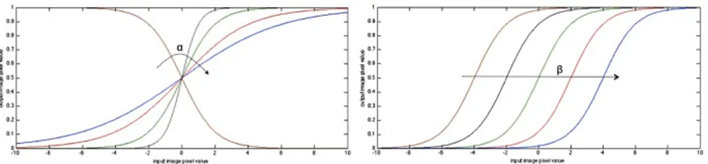
some preprocessed version. In the implemented algorithms, the feature image is computed as function of the gradient magnitude (see sec. 1.2.1) which is passed to a sigmoid ﬁlter. The Sigmoid Filter requires two parameters to deﬁne the linear transformation to be applied to the sigmoid argument (α and β):

I′= (M ax− min)( 1

1 + e−(I−βα )

) + min (1.12)

where I is the intensity of the input pixel, and I′the intensity of the output pixel. In the implemented plugin, the parameters are used to intensify the diﬀerences between regions of low and high values in the speed image. In an ideal case, the speed value should be 1.0 (M ax) in the homogeneous regions of anatomical structures and the value should decay rapidly to 0.0 (min) around the edges of structures. The α parameter deﬁnes the width of the input intensity range, and

β deﬁnes the intensity around which the range is centered1_. _{In this way the}

1_{The heuristic for finding the values is give by (58): from the gradient magnitude image,}

K1 the minimum value along the contour of the anatomical structure to be segmented, and K2 an average value of the gradient magnitude in the middle of the structure; the suggested value for β is (K1+K2)/2 while the suggested value for α is (K2-K1)/6

(46)

Figure 1.4: Sigmoid filter transform function - Intensity transform function

of sigmoid ﬁlter: eﬀect of α (a) and β (b) parameters

propagation speed of the front will be very low close to high image gradients while it will move rather fast in low gradient areas. This arrangement will make the contour propagate until it reaches the edges of anatomical structures in the image and then slow down in front of those edges.

Shape detection algorithm

The shape detection algorithm implementation, based on (67), uses the itk::Shape Detection Level-Set Image Filter. Contour evolution is guided by two terms: a propagation P term based on the feature image and a curvature-based term Z. The latter acts as a smoothing term where areas of high curvature, assumed to be due to noise, are smoothed out. Scaling parameters are used to control the tradeoff between the expansion term and the smoothing term. This filter so ex-pects two inputs, the first being an initial level-set in the form of an itk::Image, and the second being the feature image. The initial level-set is provided using, as proposed in (58), a FastMarchingImageFilter (with a constant speed) as the distance function with a set of user-provided seeds. Once activated, the level set evolution will stop if the convergence criteria or the maximum number of iterations is reached. The convergence criteria are defined in terms of the root mean squared (RMS) change in the level set function. The evolution is said to

(47)

have converged if the RMS change is below a user-speciﬁed threshold.

Geodesic Active Contours algorithm

The Geodesic Active Contours algorithm implementation, based on (68), uses the itk::Geodesic Active Contour Level Set-Image Filter. ITK implementation (58) extends the functionality of the itk::Shape Detection Level Set Image Filter by the addition of a third advection A term which attracts the level set to the object boundaries. This ﬁlter expects two inputs: an initial level set in the form of an itk::Image, and the feature image, both given as for the Shape Detection Level Set Image Filter. Also this algorithm will stop if the convergence criteria (RMS of the change) or the maximum number of iterations is reached.

1.3.2 LS-segmentation plugin

Level set segmentation filter plugin, as the EP filter plugin, is written in Objective-C with some parts in Objective-C++, following the Model-View-Objective-Controller (MVObjective-C) paradigm (see sec. 3.2.3). The plugin architecture is divided into four different classes or-ganized as in fig. 1.5:

• LSSegmentationﬁlter, the plugin entry point; • LSSegmentationController, the controller class; • ITKLSSegmentaionFilter3D, the model class; • ITKLSImageWrapper

In contrast to the EP-ﬁlter which returns an image, LS-segmentation ﬁlter cal-culates and returns to OsiriX a region of interest (ROI). This region is obtained thresholding the level-set function at the zero level: this “binary mask” is then

(48)

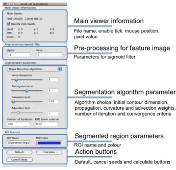
passed to an OsiriX’ ROI object and visualized. The filter implementation fol-lows the suggestion of (58), using the FastMarchingImageFilter to obtain the initial level set. This algorithm requires the user to provide a seed point from which the contour will expand. The user can actually pass not only one seed point but a set of them. A good set of seed points increases the chances of segmenting a complex object without missing parts. The use of multiple seeds also helps to reduce the amount of time needed by the front to visit a whole object and hence reduces the risk of leaks on the edges of regions visited earlier. LSsegmentation plugin panel can be divided into five functional parts (fig. 1.6):

Figure 1.5: Level Set plugin organization - Organization of Level Set

seg-mentation plugin, from OsiriX main window (top) to the image wrapper (bottom) class which takes the image to be segmented. Dashed line represent the “route” of the segmented region.

• Main viewer information, which provide information about the dataset,

mouse position and pixel value, and allows to enable the ﬁlter to collect seeds points;

• Pre-processing parameters for feature image (α and β);

• Segmentation algorithm parameters, which allows to choice segmentation

algorithm and to set its parameters;

(49)

1.4 Concluding remark

• Action buttons, to perform segmetation, to reset parameters or cancel

seeds.

Figure 1.6: Level Set plugin filter panel - Level set plugin panel divided into

ﬁve parts: Main viewer information, pre-processing for the feature image, seg-mentation algorithm parameters, segmented region parameters and action button

1.4 Concluding remark

The edge-preserving smoothing ﬁlter plugin and the Level-Set segmentation plu-gin here presented are already available in the pluplu-gin library of OsiriX software, receiving the approval from the software developer team (ﬁg. 1.7). Following the pipeline smoothing - edge enhancement - segmentation it is possible to obtain the desired ROI. A complete interaction with Penelope inkjet printer (see section 3.2) is already available: the segmented region can be transformed (using tools

(50)

provided by OsiriX) into a black and white image easily printed directly with this rapid prototyping system.

Figure 1.7: EPfilter and LSSegmentation plugins - Edge Preserving ﬁlter

(51)

Chapter 2

Indirect µ-fabrication using

PAM

2

system

Indirect Rapid Prototyping (iRP) consists in the realization of scaffolds starting from sacrificial molds built by RP systems. Because the extraction of the scaffold from the mold is a critical point of this approach, a possible solution might be low-melting point mold. In this perspective, this chapter shows the adaptation of PAM2 _{system to fabricate molds, for gelatin-based materials, using low melting} point wax. Investigation on the fabrication of agarose microstructures, based on its different gelling ability in dimethyl sulfoxide and in water, is shown at the end of this section.

2.1 PAM

2

PAM2_{(69, 70, 71, 72) is a RP system for the fabrication of scaﬀolds with a well}

deﬁned topology, using a variety of biomaterials: synthetic and natural polymers solutions, cellular suspension (bio-ink). This system is characterized by a

(52)

mod-ular architecture: various microfabrication devices can be placed on the vertical axis (z-axis) of robotic positioning system with three orthogonal axis. The x-y plane movement respect to the z-axis traces trajectories to realize a the single layer; to built other layers the microfabrication tool is moved on a ∆z distance which depends on the material used to make the scaffold. All microfabrication modules have a specific mechanical layout, independent reservoirs, specific noz-zles, and all operative parameters are controlled in an independent way. The first extrusion module, PAM (Pressure Activated Microsyringe), uses air-pressure to guide low viscosity solution extrusion. The pressure module is controlled by a pneumatic valve and the solution is extruded through glass micro-needle (with a diameter from 10 µm to 200 µm) when a pressure is applied. A second ex-trusion system, PAM2 (called also Piston Syringe), uses as driving exex-trusion force a piston. The PAM2 modulus is designed to process high viscosity solution

(with viscosity higher than 10 Pa·s). A stepper motor is used to move down

the plunger of a syringe maintaining a constant volumetric ﬂow. The solution, contained into the syringe, is deposited onto the deposition plate through cylin-drical commercial needle (with a variable diameter from 100 µm to 200 µm). Always on the z axis a support for laser pen to superﬁcially modify material, to ablate or to promote chemical reactions (such as for hydrogel polymerization). Two additional devices were purposely designed during this research to control the temperature of the reservoir (TCS - Temperature Controlled Syringe) and of the deposition plane (TDP - Temperature controlled Deposition Plate),

al-lowing PAM2 _{to work as fused deposition modeling system. After extrusion,}

due to loss of heat by conduction the physical model is formed by solidiﬁcation. This process is outstandingly well suited for materials with a low melting point and low heat conduction. Theoretically there is no limit on the type of material used. In practice, however, metals and ceramics with high melting points present

(53)

2.1 PAM2

Figure 2.1: PAM2system - PAM2system with three microfabrication modules mounted on the z-axis, and a hierarchical diagram of PAM2_{working principle. The}

box highlighted in red are investigated in this chapter

enormous problems with regard to the melting, the temperature gradient on the model, and also the required preheating of the workroom, while this approach has very good results with thermoplastic polymers.

2.1.1 PAM

2

_modules

This part of research was included in the publication (72), The PAM2 _{system: a} multilevel approach for fabrication of complex three-dimensional microstructures

Power-supply module

The power supply module was designed to provide power for all devices contained

in the PAM2 _{case (assembled during this work), but in the same time to be}

enough ﬂexible and open to allow connections (also temporary using wires) with other devices. All the PAM2_{devices are characterized by low power and diﬀerent}

(54)

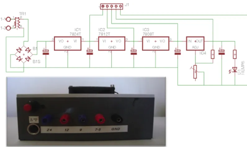
supply voltages: pressure regulator (ITV 2000, 24V, 2A), Phidgets interfaceKit, arduino duemilanove (5V), and a stepper motor (9V). The architecture of the circuit is shown in the upper part of ﬁg. 2.2, and consists of a cascade of LM78xx (7824, 7812, 7809) voltage regulators, and a LM317, an adjustable voltage regulator. A control led is provided at the end of this cascade. As shown in the bottom part of ﬁgure 2.2, connectors are also placed on the panel for an easy connection to experimental devices.

Figure 2.2: PAM2 power supply - PAM2 power supply schematic circuit

(upper part) and the external panel of the case

Temperature controlled syringe - TCS

The temperature controlled syringe (TCS) module was designed to control the temperature of inks. The TCS (ﬁg. 2.3-a) is essentially composed of an alu-minum jacket holding a commercial sterile syringe. Thanks to its design, TCS can be mount or on a position controlled mechanical stage (similar to PAM2), thus both temperature and volumetric ink ﬂow rate can be controlled, or di-rectly on the z-axis, and in this case the extrusion pressure can be controlled

(55)

2.1 PAM2

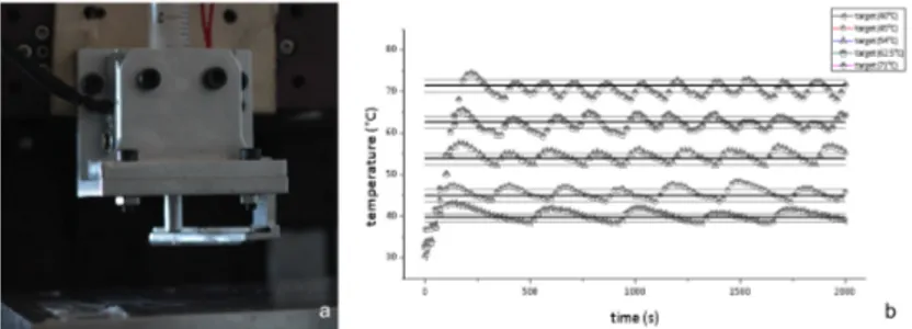
(PAM system). It is important to note that the aluminum jacket was designed to firmly hold the syringe, so no losses (in temperature or outflow resolution) occur during ink extrusion. Commercial syringes (e.g. 1, 2 and 5 ml) and cylindrical nozzles (diameter ranging from 100 µm to 500 µm) can be used with TCS. To control the performance of the TCS device, sensor and heating element are con-nected to the I/O controller (Phidgets InterfaceKit 8/8/8, Phidgets Inc, USA). The temperature control algorithm follows a closed-loop approach to maintain the target temperature in the aluminum jacket during material processing. The control algorithm was based on a step strategy: a specific threshold value (de-fined respect to the initial temperature of the device) was used to enable/disable the heating element. With this approach problems due to thermal conductance were reduced, as demonstrated by the dynamic performance (e.g. heating tem-perature range, temtem-perature error and dynamic interaction) shown in fig. 2.3-b. As shown fig. 2.3-b, once the target temperature is reached a finer temperature

Figure 2.3: TCS module - Temperature controlled syringe module mounted

directly on z-axis of PAM2 _{system (a) and its working performances}

threshold is applied by the control algorithm, and the target temperature can be maintained in time (with error of 1.5◦C respect to target value). The dynamic performance of the TCS module was recorded at diﬀerent target temperatures (i.e. from 40◦C to 70◦C). On the TCS module, in addiction, a blade can be

(56)

mounted (ﬁg. 2.3-a) to remove the excess of deposited material. The blade is took in position thanks to a magnetic ﬁxation device, it is placed at the same height of the tip of the needle, and it is thermally insulated from the rest of TCS device. Thanks to this solution (not unusual with devices that work with wax material (37)), some processing defects (see sec. 2.4) can be eliminated.

Temperature controlled deposition plane - TDP

The Temperature controlled Deposition Plane (TDP) was designed to control the temperature of the deposition plate (ﬁg. 2.4-a) of PAM2_{system. TDP operation}

is based on a Peltier cooler/heater element (or thermoelectric heat pump), a solid-state active heat pump which transfers heat from one side of the device to the other against a temperature gradient (from cold to hot), with consumption

of electrical energy. In TDP, a 10 × 10 mm Peltier element (thermoelectric

module 21.2 W, 2.9 A) is inserted between an aluminum plate (100×100 × 10

mm, used as deposition plane), an a heatsink. A fan (DC radial blower) was used to promote the heat removal from the heatsink and thus help the cooling

phase. To control the temperature of the aluminum plane, a standard NTC

Figure 2.4: TDP module - Temperature controlled deposition plate module

(a): it is possible to note the fan (on the right) to facilitate cooling of the bottom layer of the Peltier cell, and so increasing the device eﬃciency; TDP working performance (b)

(57)

2.1 PAM2

driver (L298) was used to control the direction of current in the Peltier cell switching from cooling to heating, and viceversa. All the devices were connected and controlled through a I/O board (Interface kit 8/8/8, Phidgets Inc., USA). In particular the TDP has cooling and heating rate values respectively of 1◦C·min−1 and 1.5◦C·min−1. Temperatures in the range of 18-45◦C can be controlled with maximum errors of 0.5◦C (ﬁg. 2.4-b).

PAM2 _{Camera - pCam}

pCam is an additional device of PAM2_{system to evaluate the needle-deposition}

plane distance. The pCam module consists of two parts: (a) HD camera

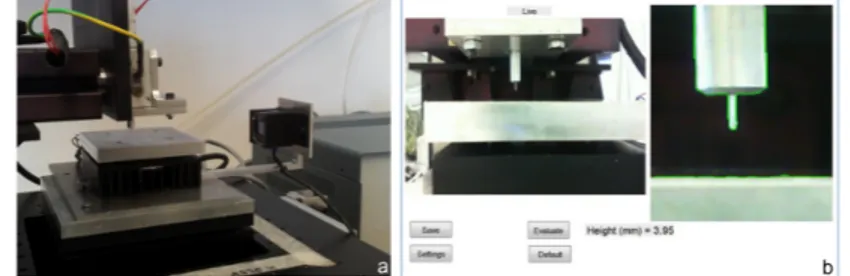
(Mi-Figure 2.5: pCam device and software - pCam: device mounted together

with TCS and TDP modules (a), and software to evaluate the needle-deposition plane distance (b)

crosoft Life Cam HD 6000) with resolution of 1280× 800 px and 66◦ diagonal ﬁeld of view, mounted on a dedicated mechanical frame fastened with the depo-sition plane, and (b) control software written in Matlab (The MathWorks, Inc.). The system (mechanical frame and software) was optimized to work with the TCS and TDP modules (ﬁg. 2.5-a).

pCam uses a HD stream video to acquire a picture of the needle and the deposition plane of PAM2 _{system, and evaluate the distance between these two}

(58)

objects using a segmentation (see sec. 1.3) approach (ﬁg. 2.5-b). An edge de-tection algorithm (Canny) is applied to the region of interest of the image. The revealed edges deﬁne two bigger regions (needle and plane), automatically recog-nized using Matlab regionprops function1_{. The distance between the bounding}

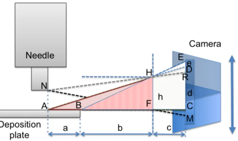
boxes of these regions is the searched distance. Because pCam uses just one camera, some preventive measurements are necessary to avoid perspective er-rors: the distance between the camera and the needle has to be in an optimal range (∼9 cm), the camera optical axis has to lie on the deposition plane. If the latter condition is satisﬁed, the needle-deposition plane distance is, from the camera point of view, equal to the distance between the needle and the edge of deposition plane, which is easy to recognize in the segmented image. To evaluate the error introduced by optical misalignment respect to the deposition plane, optical geometrical calculation were performed, following the scheme of ﬁg. 2.6. When the camera is in the right position, points A and B (the edge of deposition plane) are mapped on the same point C, so the needle - deposition plane distance AN and the needle-B distance BN are mapped into the segment

CM . Instead, when the camera is moved up (or down, for symmetry), A and B

points are mapped in the E and D points respectively: AN is mapped into the segment DR while BN is mapped into ER segment. The error introduced by

this vertical movement of the camera is the equal to ER− DR, named “e” in

the ﬁgure. It is possible to demonstrate basing on similarities between triangles (AFH-AMD and BFH-BME) that

e = h· a · c

b· (a + b) (2.1)

1_{Automatical recognition is it possible thanks to the well defined structure of the region of}

interest: high contrast respect to the background, always same lighting, relative large distance between the two objects

(59)

2.2 Microfabrication of wax material

Inserting in the 2.1 the value of a = 2 cm, b = 0.7 cm, c = 0.1 cm, for a vertical

movement h = 0.1 cm the error is equal to 3 µm. Taking in consideration

the camera technology (CMOS) this error was estimated to correspond at a maximum of 3 pixel, that is 180 µm in the ﬁnal image (60 µm each pixel). Other sources of error are discretization (∼ 20µm) and segmentation algorithm (∼ 20 µm). All these contributes aﬀects the precision of measurement system, that was found experimentally to be 30 µm (expressed as standard deviation of the mean).

Figure 2.6: pCam scheme - pCam scheme for the calculation of the perspective

error

2.2 Microfabrication of wax material

This section, after an introduction on paraﬃn waxes, chosen to realize low melt-ing point molds, describes all preliminary tests necessary to ﬁnd the process parameters for the PAM2 microfabrication system: drop formation, interaction with the deposition plate and volumetric shrinking.

(60)

2.2.1 Paraffin wax

Wax is a generic term with which people use to indicate a material with the following properties:

• workability at room temperature; • average melting point (Tm) at 44◦C; • low viscosity in fused state (5×10−3 _Pa_·s); • not soluble in water;

• hydrophobic, that means a contact angle bigger than 90◦ _{(e.g. for paraﬃn}

wax is 107◦).

From chemical point of view, waxes are a mixture of long chains of fatty acids esters (14 - 30 carbon atoms (C)) and long chain of alcohol (from 16 to 30 C) usually with one group. Waxes can be divided in low or high melting point, or, on the basis of their origin, it is possible to discriminate waxes in animal, vegetable, mineral and synthetic. Some application a wax materials to tissue engineering are listed in table 2.1.

Application Type Fabrication Technique Ref.

Porogen agent Paraﬃn Casting and leaching (73, 74) Sacriﬁcial mold Induracast⃝R

Piezo 3D printer (39, 46)

Paraﬃn Casting into a RP-made mold (44)

Table 2.1: Wax applications in Tissue Engineering

The attention of this research was focused on paraﬃn waxes. Paraﬃn waxes consist of mixtures of mainly normal alkanes (75). The amount of normal alkanes usually exceeds 75% (and may reach almost 100%), with the rest consisting of

(61)

2.2 Microfabrication of wax material

mostly iso-alkanes, cyclo-alkanes, and alkyl benzene. The molecular weight of hydrocarbons in a paraﬃn wax is in the range of about 280-560 (C20-C40), with

each specific wax having a range of about 8 to 15 carbon numbers. Melting point, a cutoff parameter for this research, increases with the number of carbon atoms (75), and restricts the choice to paraffin mainly composed by alkanes with 20 (eicosane, Tmof 36.6◦C) and 26 (exacosane, Tm56.3◦C) carbon atoms.

Experiments were performed using the Erstarr paraﬃn wax (Merck) with melting point comprised between 51-53◦C and density of 900 kg/m3_.

2.2.2 Drop Formation

One of the most important parameter of the continuous flow microfabrication technique is the distance between the needle and the deposition plane. The optimal distance, for PAM2 technique, is of the same order of magnitude of the radium of the drop formed on the tip of the needle. This value depends on the diameter and on the material of the needle, on the extrusion pressure, and on the type of extruded material. Paraffin drop formation at the tip of the needle is depicted in fig. a and a scheme of the physical system is described in fig. 2.7-b. The drop on the top of the needle grows up until its weight exceeds the surface tension forces that keep it attached to the needle, and at this point the drop falls down. The surface tension acts along the contact line between the liquid and the needle, which is a circle of diameter equal to the needle diameter Dc; it induces

a force equal to Fc= σπDc directed along the tangent of the surface liquid/gas

ad the verse is dictated by the fact that surface tension tends to “seal” the drop. In contrast to drops forming from a non-wettable nozzle, drops initially rise due to the capillary force when emerging form a wettable nozzle (the case of this research (76)) Other than surface tension, the gravity and the viscous resistance are the other forces that act the drop formation process. At the beginning the

Indirect microfabrication of biomimetic materials for locomotor tissues regeneration

University of Pisa

Faculty of Engineering

Indirect microfabrication

of biomimetic materials for

locomotor tissues regeneration

University of Pisa

Faculty of Engineering

Indirect microfabrication

of biomimetic materials for

locomotor tissues regeneration

Abstract

Acknowledgements

Contents

List of Figures

List of Tables

List of Acronyms

Introduction

Chapter 1

Image Analysis

1.1

ITK and OsiriX

1.1.1

ITK

1.1.2

OsiriX

1.2

Edge Preserving Smoothing Plugin

1.2.1

EP-plugin

1.2.2

Filters performances

1.3

Segmentation

1.3.1

Level-set segmentation

1.3.2

LS-segmentation plugin

1.4

Concluding remark

Chapter 2

Indirect µ-fabrication using

PAM

2

system

2.1

PAM

2.1.1

PAM

modules

2.2

Microfabrication of wax material

2.2.1

Paraffin wax

2.2.2

Drop Formation

_modules