ISSN: 2037-7738
GRASPA Working Papers
[online]
Web Working Papers
by
The Italian Group of Environmental Statistics
Gruppo di Ricerca per le Applicazioni della Statistica
ai Problemi Ambientali
www.graspa.org
Multivariate hidden dynamic geostatistical model
for analysing and mapping air quality data
in Apulia, Italy
Crescenza Calculli, Alessandro Fassò,
Francesco Finazzi, Alessio Pollice, Annarita Turnone
and mapping air quality data in Apulia, Italy
Crescenza Calculli⇤1, Alessandro Fass`o2, Francesco Finazzi3, Alessio Pollice4, and Annarita
Turnone5
1Italian Institute for Nuclear Physics, INFN - Bari, Via E. Orabona n. 4, 70125 Bari, Italy 2Dept. of Engineering, University of Bergamo, viale Marconi, 5 - 24044 Dalmine (BG), Italy
3Dept. of Management, Economics and Quantitative Methods, University of Bergamo, via dei Caniana 2
-24127 Bergamo (BG), Italy
4Dept. of Economics and Mathematical Methods, University of Bari, Largo Abbazia S. Scolastica, 53
-70124 Bari, Italy
5Agenzia regionale per la prevenzione e la protezione dell’ambiente, ARPA Puglia, Corso Trieste 27
-70126 Bari, Italy
Summary
In this work we propose the multivariate extension of a spatio-temporal model known in the literature and we deduce its maximum likelihood estimator based on the EM algorithm. An illustrating example concerns the joint modeling of air quality and meteorology in Apulia region, Italy. In particular a 8-variate model is fitted for daily particulate matters (PM10) and nitrogen dioxides (NO2) concentrations and six non
co-located meteorological variables, without the need of preliminary data interpolation. Some preliminary evidence of the model capability to detect a Saharan dust event is also given.
We propose an extension of a univariate hierarchical model with a Markovian latent geostatistical com-ponent, which was introduced in the literature as the dynamic spatio-temporal model. Since it is given by a Markovian sequence of spatial random fields plus a measurement error, in this paper we refer to as the hid-den dynamic geostatistical model, or HDG model. In the frame of large datasets, a semi-parametric variant of the HDG model was introduced as the fixed rank smoothing spatio-temporal random effect model (FRS-STRE). The univariate HDG has been addressed by both maximum likelihood and Bayesian techniques and some comparison studies showed its good performance in both cases.
For estimation and prediction we develop an HDG extension of the D-STEM software which is able to handle multiple variables with heterogeneous spatial supports, covariates, heterotopic monitoring networks and missing data. Uncommon in the EM literature, also the standard deviation of parameter estimates are available. In the air quality example, concentration maps and the related uncertainty maps are estimated in order to highlight the potentiality and usefulness of the proposed approach in the context of official environmental communication.
Key words: multivariate hierarchical models, spatio-temporal random effect models, D-STEM, particulate matters, nitrogen dioxides
1 Introduction
Environmental and geophysical phenomena are usually characterized by spatial and temporal variability, whose dynamics gives an opportunity to predict events and assess policies over specified areas. By means of hierarchical multivariate spatio-temporal modeling, this paper provides a framework for the analysis of air pollution phenomena which are often an emergency and one of the greatest factors of environmental risk for the human health. In particular, the European Community has defined a complete and congruent set of rules acknowledged by legislation concerning the environment of all member countries. These rules seek to standardize effective control methodologies which include monitoring, towards the quantification of the
spatial distribution of the concentration of each pollutant and the evaluation of air quality (i.e. method-ologies to measure, calculate, predict or estimate the levels of pollution in the environment). Recently, following the adoption of the new Directive 2008/50/EC of the European Parliament and of the Council of the European Union, the Italian Legislative Decree n. 155/2010 has defined new criteria for the use of evaluation methods different from measurements in fixed sites, with particular reference to modeling techniques. In this Decree potentialities of numerical models are recognized as a valuable approach to the evaluation of the air quality integrated with the analysis of measured data. Modeling techniques can also contribute to the evaluation of plans and programs for pollution reduction, as discussed in Fass`o (2013). Moreover Italian rules give local authorities the possibility to neglect air pollution excesses due to the trans-boundary transport of pollutants. In recent years, a growing number of works has shown the importance of the transboundary contribution to particulate air pollution, especially in Southern Italian regions where dust events due to intrusions of air masses coming from Saharan regions often occur (Amodio et al., 2011; Querol et al., 2004a,b). Therefore the capability to detect dust events is to be considered a relevant feature of numerical models addressing the evaluation of air quality in this area.
In the last decade univariate models for air pollution data have been extensively developed within the hierarchical modelling framework (Sahu et al., 2006; Calder, 2008; McMillan et al., 2010). As far as spatio-temporal data are concerned, univariate hierarchical models are used in several case studies. Smith et al. (2003) deal with high percentages of missing particulate matter (PM10) concentration data by a
sim-plified Expectation-Maximization (EM) algorithm. In the Bayesian framework, univariate spatio-temporal hierarchical models are proposed to account for rural/background and urban/suburban random effects on PM10 concentrations (Sahu et al., 2006), to combine monitoring data and the output from a local-scale
air pollution model for health risk assessment (Pirani et al., 2013) and to measure association of nitrogen dioxide (NO2) data with human activity in European urban areas (Shaddick et al., 2013). Multivariate
spatio-temporal data are increasingly being used in the analysis of air quality. Pollice and Jona Lasinio (2010) propose the use of a multivariate model for normalized daily concentrations of three pollutants in the Taranto area, Italy, within a Bayesian hierarchical setting including time varying weather covariates and a semi-parametric spatial covariance structure. Finazzi et al. (2013) use a three-variate model for mapping daily risk of PM10, NO2and Ozone for an heavily unbalanced monitoring network in Scotland. De Iaco
et al. (2013) implement spatio-temporal cokriging based on the linear coregionalization model (ST-LCM) to obtain prediction maps of PM10using a three-variate model which includes temperature and wind speed
in the Apulia region, Italy.
Suitable software that can handle new univariate and multivariate models with complex spatio-temporal data structures is being developed according to computational improvements. The spacetime package (Pebesma, 2012) enables the definition of data structures in space and time and allows the gstat func-tions (Pebesma, 2004) to run spatio-temporal analysis (Pebesma, 2012) in R. In the Bayesian framework, the R-INLA package (Martino and Rue, 2010) is designed for the Integrated Nested Laplace Approxima-tion (INLA) approach that represents an alternative to inference via MCMC in latent Gaussian models. The approximation of the marginal posteriors of the elements of the latent field, as well as of the model hyperparameters, is based on an efficient combination of Laplace approximations of the full conditionals and numerical integration routines. The R-INLA package provides tools for estimation and prediction within a very wide and flexible class of models ranging from (generalized) linear mixed to spatial and spatio-temporal models and is successfully used in a large amount of applications. Recently D-STEM has been proposed by Finazzi and Fass`o (2014) as a statistical package for multivariate environmental spatio-temporal data analysis and prediction. Like R-INLA this software is based on hierarchical models with latent variables but it uses the EM algorithm for model estimation. D-STEM has been successfully tested with various data structures and in several case studies: at the urban scale (Fass`o, 2013) for assessing traffic policies in Milan, Italy; at the country scale (Finazzi et al., 2013) for evaluating multi-variable air quality indexes in Scotland; and at the continental scale (Fass`o and Finazzi, 2013), considering a large data set of both ground level and remote sensing data over Europe.
In this work we propose to use the EM algorithm for the maximum likelihood estimation of a multi-variate extension of the unimulti-variate dynamic space–time model introduced by Huang and Cressie (1996). Considering snow precipitation, they focus on spatial optimal prediction and propose a simplified method-of-moment estimate which assumes no measurement errors in the response. In this paper we refer to this model as the hidden dynamic geostatistical (HDG) model, since it is given by a Markovian sequence of spatial random fields plus a measurement error. In a large comparison study Huang et al. (2007) conclude that “In terms of computation and the ability to handle large space–time data sets, a separable and flex-ible model, such as our Model I (HDG), would be the choice”. Here parameter estimation is performed using numerical optimization of the log-likelihood, assuming the measurement error variance to be known. Along these lines, considering large datasets such as global CO2on a regular grid, Katzfuss and Cressie
(2011) face the course of dimensionality by fixed rank smoothing (FRS) and a version of HDG called spatio-temporal random effects (STRE) model. The authors propose an EM estimation algorithm which is quite similar to the one in Fass`o and Finazzi (2011), but they do not use a spatial covariance model for the latent component. In a fully Bayesian frame, the same authors (Katzfuss and Cressie, 2012) pro-vide the previous STRE-FRS model with a set of appropriate priors and compare their performances in a simulation study. Cameletti et al. (2011) consider the STRE-FRS model for air quality assessment in the Piemonte Region, Italy, and compare its performance with five alternative models, including non separable covariance models. They conclude that “Model C (HDG) is the only three-star predictor: this suggests that, in our case study, a model with a complex hierarchical structure is globally preferable to one with a complex spatio-temporal covariance function”. References to the previous use of models similar to the one we propose include Cameletti et al. (2013) who consider INLA-SPDE estimation for the Piemonte dataset and Gelfand et al. (2005) who utilize a multivariate dynamic spatial models to analyze precipitations and temperatures in Colorado (USA). The latter is similar to the multivariate HDG model, but it is based a fixed random walk dynamics rather than on the more flexible Markovian one.
Here we do not enter in the unfruitful discussion about full Bayesian versus maximum likelihood estima-tion. Rather we consider HDG a popular model and the EM algorithm a valuable estimation computational tool, which is still being enriched with new features, as for example constrained estimation (Holmes, 2013) and missingness in the covariates (Naranjo et al., 2013). Hence, in this work we develop the extension of the D-STEM software (Finazzi and Fass`o, 2014) for estimation and prediction of the multivariate HDG model with missing data and non co-located monitoring networks. The illustrating example concerns the concentrations of PM10and NO2and the measurements of five meteorological variables in the Apulia
re-gion, Italy. As it is often the case, pollution and meteorological information come from two monitoring networks, differing in the number of stations and their spatial locations. In particular, we consider both pollutant concentrations and meteorological variables as response variables in the model formulation, so that no data imputation or interpolation is required. The Kriging approach is then applied with the esti-mated model for daily mapping pollutant concentrations over the study region. Although not reported in this paper, the model can also be used to obtain daily maps of the meteorological variables.
The remaining part of the paper is structured as follows: the whole Section 2 is dedicated to the defini-tion of the multivariate HDG model and its maximum likelihood estimadefini-tion by means of the EM algorithm. The use of this model is illustrated in Section 3 through a case study concerning air pollution in the Apulia region, Italy. The results of estimation and mapping procedures are discussed in Section 3.1 with particular reference to a Saharan dust event. Finally, Section 4 provides the main concluding considerations and some remarks on the proposed approach.
2 The multivariate hidden dynamic geostatistical model
Let y(s, t) = (y1(s, t), . . . , yq(s, t))0 be the q-variate response variable at site s 2 D ⇢ R2and discrete
hidden dynamic geostatistical (HDG) model if it is defined by y(s, t) = X (s, t) + Xz(s, t) Az(s, t) + "(s, t)
z(s, t) = Gz(s, t 1) + ⌘(s, t) (1)
where z(s, t) = (z1(s, t), ..., zp(s, t))0 is a latent random variable with Markovian dynamics, ⌘(s, t) =
(⌘1(s, t), . . . , ⌘p(s, t))0is the spatially correlated temporal innovation while "(s, t) = ("1(s, t), ..., "q(s, t))0
is the random measurement error.
In general, p and q can be different, but the case p = q is considered here, as discussed in subsection 2.1. In Equation (1) ⌘(s, t) is a Gaussian process, namely ⌘(s, t) ⇠ GPq(0, ), with matrix correlation
function given by
= V⇢(ks s0k; ✓, ⌫)
where V is a valid q dimensional correlation matrix with elements vi,j, while
⇢(ks s0k; ✓, ⌫) = 1 ˜(⌫)2⌫ 1 ✓p 2⌫ks s0k ✓ ◆⌫ K⌫ ✓p 2⌫ks s0k ✓ ◆ (2) is the Mat´ern spatial covariance function. In particular, ks s0k is the distance between two generic spatial
locations, ✓ > 0 and ⌫ > 0 are parameters, ˜ is the gamma function and K⌫is the modified Bessel function
of the second kind. The range parameter ✓ is here assumed unknown while the smoothing parameter ⌫ is fixed. The measurement errors "i(s, t)are independent and white noise in space and time but each variable
retains its own variance, namely Var("(s, t)) = diag( 2) =diag( 2
1, ..., q2).
The fixed effect design matrix X (s, t) is such that each observed variable yi(s, t)can be related to bi
covariates. In particular
X (s, t) =blockdiag (x ,1(s, t), ..., x ,q(s, t))
where blockdiag is the block diagonal operator and x ,i(s, t), i = 1, ..., q are 1⇥bivectors, b1+...+bq = b.
Instead, the random effect design matrix
Xz(s, t) =diag (xz,1(s, t), ..., xz,q(s, t))
is a q ⇥ q diagonal matrix, set to the identity matrix in the present simple case. Finally A = diag (↵1, ..., ↵q), = 01, ..., q0
0
, where i= ( i,1, ..., i,bi)
0are vectors of unknown
coefficients, while G =diag (g1, ...gq)is the diagonal transition matrix.
The parameter set to be estimated is then given by = ↵, , 2, G, V, ✓
where, with abuse of notation, we use V for its lower triangular submatrix and G = (g1, ...gq), which
define the unique parameters to be estimated for these two matrices.
2.1 Comments on some features of the multivariate HDG model
The assumption p = q is made here to ease model interpretability, as it allows to univocally relate each observed variable yi(s, t)to one and only one latent component zi(s, t). In general this assumption is not
necessary, another important special case being the common factor latent model with p = 1: sharing the same z component among different yi’s is useful for example in data fusion, see e.g. Fass`o and Finazzi
(2013) and Berrocal et al. (2012).
Under the assumption that the transition matrix G is diagonal, the q dimensional VAR model for z(s, t) in (1) may be splitted into q separated equations, nonetheless the components zi(s, t)are correlated, due to
the correlation among the components of ⌘tgiven by matrix V. Yule-Walker recursive formulas relating
the auto-covariance matrices of z(s, t) and the variance covariance matrix of the innovation ⌘tare easily
obtained, see e.g. Huang and Cressie (1996).
The HDG model is shown to have a multiplicative separable covariance function by Cameletti et al. (2011). If one prefers additive separability, this is obtained by a variant of HDG model in which the product a (s, t) = Xz(s, t) Az (s, t)is substituted by the sum
a (s, t) = X⇣(s, t) ⇣ (t) + X⌘(s, t) ⌘ (s, t) (3)
where ⇣ (t) is a purely temporal Markovian process common to all locations, ⌘ (s, t) is an iid sequence of random fields defined as in model (1), X⌘(s, t)and X⇣(s, t) are suitable known quantities. This is
essentially the model considered in the original version of D-STEM software.
In the following Apulian case study the identity matrix is a natural choice for Xz(s, t) with p =
q. Nevertheless the role of a more general random effect design matrix Xz(s, t) can be quite relevant.
When xz,i(s, t), i = 1, ..., q are strictu sensu covariates, then the respective zi(s, t) can be seen as the
corresponding spatio-temporal varying coefficients. Moreover, following a semiparametric approach, if ⌘ (s, t) in (1) is white noise in space and time and xz,i(s, t) are some appropriate basis functions, e.g.
splines, the fixed rank smoothing spatio-temporal random effects (FRS-STRE) model of Katzfuss and Cressie (2011) is obtained.
2.2 Complete-data likelihood function
Suppose that the q variables are observed at the sets of spatial locations Si ={si,1, ...si,ni}, i = 1, ..., q and let yi(Si, t) =stack (yi(si,1, t), ..., yi(si,ni, t)), where stack is the stacking operator. Then, for each time t, the following n ⇥ 1 observation vector is obtained
yt = y1(S1, t)0, ..., yq(Sq, t)0 0 (4)
with n = n1+ ... + nq. In general, Si 6= Sj, that is, each variable can be observed at a different set
of spatial locations. Moreover, the vector ytmay include missing values. Model (1) can be given the
following representation yt = µt+ "t
µt = Xt + XtzAz˜ t
zt = Gz˜ t 1+ ⌘t
(5) with Xt =blockdiag (X ,1(S1, t), ..., X ,q(Sq, t)) ,where X ,i(Si, t) =stack (x ,i(si,1, t), ..., x ,i(si,ni, t)) , and Xz
t =blockdiag (Xz,1(S1, t), ..., Xz,q(Sq, t)) ,where Xz,i(Si, t) =diag (xz,i(s1,1, t), ..., xz,i(s1,ni, t)), for i = 1, ..., q. Vectors µt, zt, ⌘tand "tare defined as ytin (4). Finally ˜A =blockdiag ↵1In1, ..., ↵qInq and ˜G =blockdiag g1In1, ..., gqInq , where Iniis the identity matrix of dimension ni. In order to define the complete-data log-likelihood function, notice that the following Gaussian distributions are implied by the model structure:
yt| zt ⇠ Nn(µt, ⌃") zt| zt 1 ⇠ Nn ⇣ ˜ Gzt 1, ⌃⌘ ⌘ z0 ⇠ Nn(µ0, ⌃0)
with variance-covariance matrices given by ⌃"=blockdiag 12In1, ...,
2
qInq and ⌃⌘= (vi,j⇢ (Hij))i,j=1,...,q,
where Hij = d (Si,Sj) is the distance matrix between the spatial locations in Si and in Sj, and the
With this notation, the complete-data log-likelihood function for observations Y = {y1, ..., yT} and Z ={z0, z1, ..., zT} is given by: 2l ( ; Y, Z) = T log|⌃"| + T P t=1 e0 t⌃"1et + log|⌃0| + (z0 µ0)0⌃01(z0 µ0) +T log|⌃⌘| + T P t=1 ⇣ zt Gz˜ t 1 ⌘0 ⌃ 1 ⌘ ⇣ zt Gz˜ t 1 ⌘
where et = yt µt. Notice that, due to the hierarchical structure of HDG model, l ( ; Y, Z) may be
written as l ( ) = l ( 1) + l (µ0, ⌃0) + l ( 2)where 1 = ↵, , 2, G and 2 = (V, ✓), reducing
the optimization dimensionality in the maximization step of the EM algorithm.
2.3 Missing data handling
In order to deal with missing data, the observation vector at time t, yt, is partitioned as
˜ yt= ✓⇣ y(1)t ⌘0 ,⇣y(2)t ⌘0◆0 , where y(1)
t = Ltytis the sub-vector of non-missing data at time t and Ltis the elimination matrix. Vector
˜
ytis thus a permutation of ytand yt= Dt˜yt, with Dtthe commutation matrix. In the sequel, given bt
a generic n ⇥ 1 vector and Bta generic n ⇥ n matrix at time t, b(1)t and B (1)
t will stand for Ltbtand
LtBtL0t, respectively. On the other hand, if Btis a n ⇥ m matrix, then B(1)t = LtBt. Finally, 0n and
0n⇥mwill be used to define the n ⇥ 1 vector and the n ⇥ m matrix of all zeros, respectively.
The first equation in (5) becomes y(l)
t = µ
(l) t + "
(l)
t , l = 1, 2 and the variance-covariance matrix of the
permuted errors is conformably partitioned, namely: Var " (1) t "(2)t ! = ✓ R11 R12 R012 R22 ◆
Since ⌃"is diagonal, it follows that R11and R22are diagonal matrices while R12= 0(n ut)⇥ut, with ut the number of non-missing data at time t.
2.4 EM algorithm
The EM algorithm is considered here to obtain the maximum likelihood estimate of the model parameter set . The algorithm is known to be based on the iteration of an expectation step and a maximization step. The expectation step amounts at computing Q , hmi = E hmi⇥ 2l ( ; Y, Z)| Y(1)⇤where
Y(1) =ny(1) 1 , ..., y
(1) T
o
, and the maximization step, namely hm+1i = arg maxQ , hmi , gives the
updating formulas for the model parameters. A full derivation of the updating formulas is given in the appendix. Interestingly, for the non geostatistical part of , namely 1 = ↵, , 2, G , the updating
formulas are available in closed form, as follows: ↵hm+1ii = T P t=1 tr ˜Ii⇣y(1) t X ,(1) t ⌘ ⇣ Xz,(1)t zTt ⌘0 T P t=1 tr˜IiXz,(1) t ⇣ zT t zTt 0 + PT t ⌘ ⇣ Xz,(1)t ⌘0 , i = 1, ..., q hm+1i = " T X t=1 ⇣ Xt,(1) ⌘0 Xt,(1) # 1 T X t=1 ⇣ Xt,(1) ⌘0h y(1)t X z,(1) t Az˜ T t i! 2 i hm+1i = 1 niT tr " ˜Ii T X t=1 ✓ ⌦(1)t 0ut⇥(n ut) 0ut⇥(n ut) R22 ◆# , i = 1, ..., q ghm+1ii = trh˜IiS10i trh˜IiS00i , i = 1, ..., q µhmi0 = zT0. where zT
t = E zt| Y(1) , PTt =Var zt| Y(1) and PTt,t 1=Cov zt, zt 1| Y(1) denote the output
of the Kalman smoother, S10 = PTt=1zTt zTt 1 0 + PT t,t 1and S00 =PTt=1zTt 1 zTt 1 0 + PT t 1are
the well known EM second moments (see e.g. Shumway and Stoffer (2010)), matrix ⌦(1)
t is given in the
Appendix and ˜Iiis a selector matrix defined by
˜Ii =diag 0 B @00n1, ..., i th position z}|{ 10ni , ..., 0 0 nq 1 C A
and used to set to zero all the diagonal elements of the matrix pre-multiplied by ˜Iiand not related to the i-th
variable. Also notice that µ0is not considered as a model parameter but it is needed to start the Kalman
recursion.
Finally, the geostatistical model parameters 2 = (V, ✓)are updated through numerical optimization.
In particular n
Vhm+1i, ✓hm+1io= arg max
V,✓ T log|⌃⌘| + tr h ⌃⌘1 ⇣ S11 S10G˜0 GS˜ 0 10+ ˜GS00G˜0 ⌘i (6) where S11=PTt=1zTt zTt 0 + PTt.
Starting from an initial value h0i for the model parameter set, the EM algorithm is iterated until
convergence, that is, until the observed data log-likelihood or the elements of the model parameters stop changing significantly.
2.5 Mapping with the HDG model
Given the maximum likelihood estimates of the parameter set , predictions of the i-th response at new sites S0and time t = 1, ..., T are obtained:
ˆ
yi(S0, t) = X ,i(S0, t) ˆi+ Xz,i(S0, t) ˆAi(S0)zT,it (S0) (7)
while the variance-covariance matrix of ˆyi(S0, t)is given by
⌃yˆi(S0, t) = ˆAi(S0)
2X
where zT,i
t (S0)and PT,it,t 1(S0)are the Kalman smoother outputs extended over sites S0and for the i-th
variable while ˆAi(S0) = ˆ↵iI|S0|. If S0overlays the entire region D as a fine regular grid, ˆyi(S0, t)allows to draw a map and the ordered collection
ˆ
Yi(S0) ={ˆyi(S0, 1), . . . , ˆyi(S0, T )} (9)
represents a dynamic map for the i-th variable.
3 The Apulia case study
The methodology discussed in the previous sections is applied to air quality data collected in Apulia for jointly analyzing and mapping concentrations of two troublesome pollutants over the study area: PM10
and NO2. Apulia (South-eastern Italy) is a wide, mostly coastal, territory with a high demographic density.
The region is characterized by some of the highest environmental risk areas in Italy, deeply investigated for the presence of several industrial activities (as petrochemical plants, oil refineries, navy arsenals, electric power plants) near urban centers (Martuzzi et al., 2002). It is well known that high concentrations of both PM10and NO2are measured in those urban areas characterized by high population density, heavy traffic
and industries. Whereas particulate matter and the exceedance of the related limiting values have attracted considerable public attention during the last years, the NO2 problem is a relatively new one becoming
mature through the introduction of new European limiting values in 2010 (EU Directive 2008/50/EC). We analyze the daily average concentrations (in µg/m3) of both PM
10and NO2and the measurements of some
meteorological variables that may drive the pollutant diffusion and advection. Pollutant concentrations and the meteorological data are provided by the Apulia Region Environmental Protection Agency (ARPA Puglia) and by the Agrometeorological Service of the Apulia region (ASSOCODIPUGLIA), respectively. We consider a three months study period (T = 92 days) corresponding to the summer season 2012 (from 1stJuly to 30thSeptember). This period was characterized by high temperatures and an event of intrusion
of long range transported air mass from the African continent, with a large number of monitoring sites exceeding the daily PM10limit value of 50 µg/m3(according to the Legislative Decree 155/2010). The
focus on this time period is particularly relevant as the Italian law gives local authorities the possibility to neglect air pollution excesses due to the transboundary transport that was recently shown to provide a substantial contribution to particulate air pollution in Southern Italian regions, where intrusion of air masses coming from Saharan dust events often occurs (Amodio et al., 2011; Querol et al., 2004a,b).
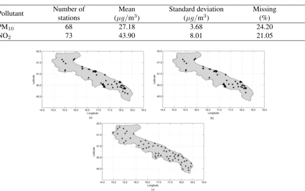
PM10 and NO2 concentrations come respectively from 73 and 68 monitoring sensors of the Apulia
multipollutant air quality network. Figures 1(a) - 1(b) show the spatial distribution of the two pollutants measuring sites. The missing data rates for each pollutant are reported in Table 1. Meteorological data come from 58 stations (Figure 1(c)) and no missing data occur in the period. We consider the daily average temperature (TEMP, in °C), relative humidity (RH, in %), atmospheric pressure (AP, in hPa), wind speed (WINDs, in m/s), east-west (WINDu, in m/s) and north-south wind component (WINDv, in m/s).
Precipitations are not considered, due to the lack of rainy days except for a short rainfall in the last week of July. Pollutant concentrations and meteorological variables are integrated by a set of time invariant covariates as population counts (pop), monitoring station coordinates (lat and lon, UTM coordinates in km) and land elevation (elev, in m). Population data are considered as a proxy of pollution emissions and are drawn from the LandScanTMambient population count database, updated to the year 2008 (Bhaduri
et al., 2007), which provides global population data with approximately 1 km resolution (30”⇥ 30”). Land elevation data come from the GTOPO30 global digital elevation model (DEM) with a horizontal grid spacing of 30 arc-seconds (approximately 1 kilometer).
Pollutant concentrations and meteorological data are obtained by non co-located monitoring networks (see Figure 1), giving an example of heterotopic spatial data, where different variables are observed at different locations (Wackernagel, 2003). In order to exploit the meteorological information avoiding data
Table 1 Summary statistics of the pollutant concentrations from 1stJul to 30thSept, 2012.
Pollutant Number ofstations (µg/mMean3) Standard deviation(µg/m3) Missing(%)
PM10 68 27.18 3.68 24.20
NO2 73 43.90 8.01 21.05
Fig. 1 Spatial distribution of the Apulia region air quality network: (a) NO2(73 sites); (b) PM10(68 sites). Locations
of the meteorological network sites: (c) meteorological stations (58 sites).
interpolation, we choose to consider both air quality and meteorological variables as a 8-dimensional re-sponse vector. Traffic-type stations are excluded from the analysis to avoid possible overestimation of the concentration of the two pollutants over the entire region, as traffic and road data are not currently available.
Maximum likelihood parameter estimation and spatial predictions for the multivariate HDG model are implemented by an extension of the D-STEM software previously introduced by Finazzi and Fass`o (2014), based on the EM algorithm which reaches convergence even when the number of parameters to be esti-mated is high as in the case study. Model estimations and mapping are performed on an Intel(R) Core(TM) i3- 2370M CPU laptop, with 2.40 GHz and 8GB RAM. The estimation time is ⇠ 27 minutes and the EM algorithm takes 42 iterations to converge.
3.1 Estimation and mapping results
In this Section we report the results of the EM maximum likelihood estimation of the multivariate HDG model for the case study. Preliminary data analysis (not reported, but available from the authors upon request) led to log-transform pollutant concentrations to reduce heteroskedasticity and long tails in the data distributions. All response variables and covariates were also standardized in order to improve numerical stability and an simplify the comparison between the parameter values across pollutants and meteorological variables.
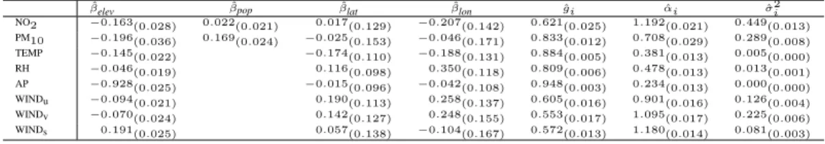
Table 2 reports the maximum likelihood estimates of the parameters in . The estimated ˆ-coefficients suitably describe the physics of air pollution. As expected land elevation (elev) has a significant effect in reducing both PM10and NO2 concentrations. A positive relationship can be seen between the covariate
Table 2 Estimated parameters for the multivariate HDG model. Standard deviations in parentheses.
ˆelev ˆpop ˆlat ˆlon ˆgi ↵iˆ ˆ2i
NO2 0.163(0.028) 0.022(0.021) 0.017(0.129) 0.207(0.142) 0.621(0.025) 1.192(0.021) 0.449(0.013) PM10 0.196(0.036) 0.169(0.024) 0.025(0.153) 0.046(0.171) 0.833(0.012) 0.708(0.029) 0.289(0.008) TEMP 0.145(0.022) 0.174(0.110) 0.188(0.131) 0.884(0.005) 0.381(0.013) 0.005(0.000) RH 0.046(0.019) 0.116(0.098) 0.350(0.118) 0.809(0.006) 0.478(0.013) 0.013(0.001) AP 0.928(0.025) 0.015(0.096) 0.042(0.108) 0.948(0.003) 0.234(0.013) 0.000(0.000) WINDu 0.094(0.021) 0.190(0.113) 0.258(0.137) 0.605(0.016) 0.901(0.016) 0.126(0.004) WINDv 0.070(0.024) 0.142(0.127) 0.248(0.155) 0.553(0.017) 1.095(0.017) 0.225(0.006) WINDs 0.191(0.025) 0.057(0.138) 0.104(0.167) 0.572(0.013) 1.180(0.014) 0.081(0.003)
Table 3 Estimated ˆVcorrelation matrix of the multivariate HDG model. Standard deviations in parentheses.
NO2 PM10 TEMP RH AP WINDu WINDv WINDs
NO2 1.00 0.637(0.033) 0.021(0.073) 0.123(0.057) 0.578(0.094) 0.210(0.031) 0.181(0.026) 0.299(0.021) PM10 1.00 0.223(0.141) 0.089(0.117) 0.001(0.231) 0.270(0.065) 0.002(0.057) 0.515(0.041) TEMP 1.00 0.617(0.079) 0.000(0.192) 0.063(0.068) 0.094(0.056) 0.057(0.044) RH 1.00 0.004(0.163) 0.042(0.056) 0.003(0.046) 0.016(0.036) AP 1.00 0.155(0.102) 0.047(0.087) 0.191(0.064) WINDu 1.00 0.132(0.026) 0.082(0.022) WINDv 1.00 0.524(0.014) WINDs 1.00
pop and PM10, showing higher concentrations of this pollutant in most populated areas. The signs of
esti-mated coefficients related to meteorological variables are also in line with their physical behavior, e.g. the estimated ˆelevis negative for the TEMP, RH and AP responses, representing the tendency of these
vari-ables to decrease with growing altitude. Notice the systematic higher estimated sd’s of the effects of the lon coordinate with respect to lat, possibly highlighting the presence of anisotropy due to the stretched shape characterizing the observation area. The analysis of the ˆgi-values suggests that response variables have
specific temporal dynamics. In particular, the PM10 has a slower temporal dynamics compared to NO2,
while directional wind components are characterized by lower persistence. Estimates of ↵i’s account for
the importance of the spatio-temporal interaction term z(s, t) and show an inverse proportional compen-sation behavior with ˆgi’s. The measurement errors ˆ2i are higher for NO2than PM10and generally lower
for all meteorological variables, except for the North-South wind component, corresponding to peaks of intensity of winds blowing from North-East over the study area. The estimated parameter ˆ✓ represents the range (in km) of the exponential spatial correlation (⌫ = 1/2) common to all response variables and expressed by the latent random vector ⌘(s, t). It amounts to 182.08 km (sd = 4.313), implying a smooth spatial behavior. The estimated matrix ˆVis reported in Table 3, representing the cross-correlations of the elements of ⌘(s, t). A positive correlation between the two pollutants is noticeable, legitimizing the choice of the multivariate model considering the two pollutants altogether.
In order to evaluate the predictive capability of the multivariate HDG model, a leave one site out cross-validation (CV) is used, following the approach proposed in Fass`o et al. (2007). The procedure consists in recursively estimating the multivariate HDG model removing one site at a time, then predicting con-centrations of both pollutants at the removed site for the 92 time points. Cross-validation mean squared errors (CMSE) for the two pollutants, obtained averaging the squared residuals for each day and site, are respectively CMSENO2= 0.663 and CMSEPM10= 0.565, confirming the different predictive capability of the multivariate HDG model shown by the estimated measurement errors ˆ2
i in Table 2.
The descriptive capability of the multivariate HDG model is exemplified focusing on a specific atmo-spheric event by the dynamic maps ˆYN O2(S0)and ˆYP M10(S0)(see Equation 9, Section 2.5) evaluated over a fine regular grid S0 with high spatial resolution (1km ⇥ km approximatively) within the Apulia
boundaries. Maps in Figure 2 show the estimated daily average concentrations of PM10and NO2and the
Fig. 2 Estimated NO2concentration and standard deviation (top and bottom left) and estimated PM10concentration
and standard deviation (top and bottom right) for the dust day (September 29, 2012) over the Apulia region. The ‘+’ symbol represents the air quality network stations.
Fig. 3 Log-transformed standardized concentrations of the two pollutants at the Campi Salentina monitoring station on 21-30 September 2012: observed (solid lines), model predictions (dotted) and CV predictions (dashed).
satellite images (Draxler and Rolph, 2011) and synoptic analysis indicate a probable advection of African dust particles over the the Apulia region reaching its maximum on 29 September. Such events do not have a constant evolution in time and can involve only part of the area under consideration, due to its geographical configuration. Maps obtained by the procedure defined in Section 2.5 focused on the dust event show that on 29 September the estimated PM10concentrations exceed the threshold of 50 µg/m3over the Salento
peninsula (south of Apulia) and in the metropolitan areas of Taranto, Bari and Foggia. NO2 estimated
concentrations are not as high, proving that this pollutant is not as affected by the advection of dust par-ticles. Uncertainties related to both pollutant maps are quite small, excluding the unmonitored areas and those along the borders of the region. A further example of the multivariate HDG model capabilities is obtained comparing observed concentrations of the two pollutants with model predictions obtained as in
(9) and CV predictions at the Campi Salentina monitoring station, located in the Southern part of the study area, mostly exposed to the dust event. As expected, due to the outlying character of particulate matter in these days, the model underestimates PM10. Instead, due to positive cross correlation among pollutants, it
overestimates NO2as shown in Figure 3. This behavior can be considered as the basis to define a statistical
detector of dust events.
4 Conclusion and discussion
In this work we propose the maximum likelihood estimation of a multivariate spatio-temporal model which can be used for the analysis and mapping of air quality data. We consider a model specification based on a first order auto-regressive spatial component to jointly model spatial and temporal dependencies. The use of the multivariate HDG model is illustrated for a case study concerning air quality over the Apulia region, Italy. Concentrations of NO2and PM10and a set of meteorological variables are considered in a
multivariate setting. The proposed approach allows to handle missing data and non co-located monitoring networks in a natural way. For the purpose we extend the D-STEM software based on the EM algorithm giving model parameter estimates, dynamic maps and cross-validation results.
It is worth pointing out that the HDG model provides a flexible structure for the analysis of air quality in several data frameworks. For instance, this modeling approach could be used for the temporal forecasting of concentration levels possibly coupled with a meteorological forecaster. A line of further investigation is related to almost real-time mapping of air quality data, obtained through daily recursive model estimation. This is accomplished considering a sliding data window of size n days in Calculli et al. (2014). The case study suggests that joint HDG modeling of particulate and gaseous air pollutants may be used to detect dust events on a statistical basis and further research on this subject is needed to devise statistical methods for transboundary adjustment of particulate matters. The availability of traffic and road data would allow the integration of the case study data base with traffic-type sensor pollutant concentration data, avoiding possible overestimation of the anthropogenic contribution to NO2and PM10pollution over
the entire region.
Acknowledgements. The authors thank ASSOCODIPUGLIA - Associazione Regionale dei Consorzi di Difesa della Puglia for providing the meteorological data. The analysis utilized the LandScanTMhigh resolution global population
data set copyrighted by UT-Battelle, LLC, operator of Oak Ridge National Laboratory under contract DE-AC05-00OR22725 with the US Department of Energy. The US Government has certain rights on this data set. Neither UT-Battelle, LLC, nor the US Department of Energy, nor any of their employees, makes any warranty, express or implied, or assumes any legal liability or responsibility for the accuracy, completeness, or usefulness of the data set. Finazzi was funded for this work through the FIRB2012 project “Statistical modelling of environmental phenomena: pollution, meteorology, health and their interactions” (RBFR12URQJ).
References
Amodio M, Andriani E, Angiuli L, Assennato G, De Gennaro G, Gilio AD, Giua R, Intini M, Menegotto M, Nocioni A, Palmisani J, Perrone MR, Placentino CM, Tutino M, 2011. Chemical characterization of PM in the Apulia region: local and long-range transport contributions to particulate matter. Boreal Environmental Research16: 251–261.
Berrocal V, Gelfand A, Holland D, 2012. Space-time data fusion under error in computer model output: an application to modeling air quality. Biometrics68: 837–848.
Bhaduri B, Bright E, Coleman P, Urban M, 2007. Landscan USA: a high resolution geospatial and temporal modeling approach for population distribution and dynamics. GeoJournal69: 103–117.
Calculli C, Turnone A, Finazzi F, Pollice A, Morabito A, 2014. Model based spatio-temporal analysis and mapping of Apulia air quality data. Proceedings of 1st International Conference on Atmospheric Dust, Castellaneta Marina - Italy, June 1-6, 2014.
Calder CA, 2008. A dynamic process convolution approach to modeling ambient particulate matter con-centrations. Environmetrics19(1): 39–48.
Cameletti M, Ignaccolo R, Bande S, 2011. Comparing spatio-temporal models for particulate matter in Piemonte. Environmetrics22(8): 985–996.
Cameletti M, Lindgren F, Simpson D, Rue H, 2013. Spatio-temporal modeling of particulate matter con-centration through the SPDE approach. AStA Advances in Statistical Analysis97(2): 109–131.
De Iaco S, Palma M, Posa D, 2013. Prediction of particle pollution through spatio-temporal multivariate geostatistical analysis. AStA Advances in Statistical Analysis97(2): 133–150.
Draxler R, Rolph GD, 2011. HYSPLIT (HYbrid Single-Particle Lagrangian Integrated Trajectory). NOAA Air Resources Laboratory, Silver Spring, MD. Available at: http://ready.arl.noaa.gov/ HYSPLIT.php.
Fass`o A, 2013. Statistical assessment of air quality interventions. Stochastic Environmental Research and Risk Assessment27(7): 1651–1660.
Fass`o A, Cameletti M, Nicolis O, 2007. Air quality monitoring using heterogeneous networks. Environ-metrics18(3): 245–264.
Fass`o A, Finazzi F, 2011. Maximum likelihood estimation of the dynamic coregionalization model with heterotropic data. Environmetrics22(6): 735–748.
Fass`o A, Finazzi F, 2013. A varying coefficients space-time model for ground and satellite air quality data over Europe. Statistica & Applicazioni, Special online issue : 45–56.
Finazzi F, Fass`o A, 2014. D-STEM: A software for the analysis and mapping of environmental space-time variables. Journal of Statistical Software. Accepted.
Finazzi F, Scott EM, Fass`o A, 2013. A model-based framework for air quality indices and population risk evaluation, with an application to the analysis of Scottish air quality data. Journal of The Royal Statistical Society: Series C62(2): 287–308.
Gelfand AE, Banerjee S, Gamerman D, 2005. Spatial process modelling for univariate and multivariate dynamic spatial data. Environmetrics16(5): 465–479.
Holmes E, 2013. Derivation of an EM algorithm for constrained and unconstrained multivariate autore-gressive state-space (MARSS) models. arXiv:1302.3919v1 .
Huang H, Cressie N, 1996. Spatio-temporal prediction of snow equivalent using the Kalman filter. Com-putational Statistics and Data Analysis22: 159–175.
Huang H, Martinez F, Mateu J, Montes F, 2007. Model comparison and selection for stationary space–time models. Computational Statistics and Data Analysis51: 4577–4596.
Katzfuss M, Cressie N, 2011. Spatio-temporal smoothing and EM estimation for massive remote-sensing data sets. Journal of Time Series Analysis4(1): 430–446.
Katzfuss M, Cressie N, 2012. Bayesian hierarchical spatio-temporal smoothing for very large datasets. Environmetrics23(1): 94–107.
Martino S, Rue H, 2010. Implementing approximate Bayesian inference using Integrated Nested Laplace Approximation: a manual for the INLA program. Available at: http://www.math.ntnu.no/ hrue/GMRFsim/manual.pdf.
Martuzzi M, Mitis F, Biggeri A, Terracini B, Bertollini R, 2002. Environment and health status of the population in areas with high risk of environmental crisis in italy. Epidemilogia e Prevenzione26(6): 1–53.
McMillan N, Holland DM, Morara M, Feng J, 2010. Combining numerical model output and particulate data using Bayesian space-time modeling. Environmetrics21: 48–65.
Naranjo A, Trindade A, Casella G, 2013. Extending the state-space model to accommodate missing values in responses and covariates. Journal of the American Statistical Association108(501): 202–216. Pebesma EJ, 2004. Multivariable geostatistics in S: the gstat package. Computers & Geosciences30: 683–
691.
Pebesma EJ, 2012. spacetime: Spatio-temporal data in R. Journal of Statistical Software51(7): 1–30. Pirani M, Gulliver J, Fuller GW, Blangiardo M, 2013. Bayesian spatiotemporal modelling for the
assess-ment of short-term exposure to particle pollution in urban areas. Journal of Exposure Science & Envi-ronmental Epidemiology27: 1–9, doi: 10.1038/jes.2013.85.
Pollice A, Jona Lasinio G, 2010. A multivariate approach to the analysis of air quality in a high environ-mental risk area. Environmetrics21(7-8): 741–754.
Querol X, Alastuey A, Rodr´ıguez S, Viana MM, Art´ınano B, Salvador P, Mantilla E, Santos S, Patier R, De la Rosa J, De la Campa AS, Men´endez M, Gil JJ, 2004a. Levels of PM in rural, urban and industrial sites in Spain. The Science of Total Environment334: 359–376.
Querol X, Alastuey A, Viana MM, Rodr´ıguez S, Art´ınano B, Salvador P, Do Santos SG, Patier R, Ruiz C, De la Rosa J, De la Campa AS, Menendez M, Gil JJ, 2004b. Speciation and origin of PM10 and PM2.5 in Spain. Aerosol Science35: 1151–1172.
Sahu SK, Gelfand AE, Holland D, 2006. Spatio-temporal modeling of fine particulate matter. Journal of Agricultural Biological and Environmental Statistics11(1): 61–86.
Shaddick G, Yan H, Vienneau D, 2013. A Bayesian hierarchical model for assessing the impact of human activity on nitrogen dioxide concentrations in europe. Environmental and Ecological Statistics,20: 553– 570, doi: 10.1007/s10651-012-0234-z.
Shumway R, Stoffer D, 2010. Time series analysis and its applications, with R examples, 3rd edn. Springer, New York.
Smith RL, Kolenikov S, Cox LH, 2003. Spatio-temporal modeling of PM2.5 data with missing values. Journal of Geophysical Research108(D24), doi: 10.1029/2002JD002914.
Wackernagel H, 2003. Multivariate Geostatistics: An introduction with applications, 2nd edn. Springer, New York.
Appendix A
In this appendix a derivation of the closed form formulas of section 2.4 is given. The starting point is the following representation of the conditional expectation of the complete-data log-likelihood, or the E step:
Q⇣ , hmi⌘ = E hmi h 2l ( ; Y, Z)| Y(1)i = E hmi h E hmi h 2l ( ; Y, Z)| Y(1), Zi| Y(1)i.
In what follows let E (· | ·) ⌘ E hmi(· | ·) and Var (· | ·) ⌘ Var hmi(· | ·). Considering the inner conditional expectation, the following result holds
E⇥ 2l ( ; Y, Z)| Y(1), Z⇤= T log|⌃ "| + tr ⌃ 1 " T P t=1 ⇣ E et| Y(1), Z E et| Y(1), Z 0+Var et| Y(1), Z ⌘ + log|⌃0| + tr h ⌃01(z0 µ0) (z0 µ0) 0i +T log|⌃⌘| + tr ⌃ 1 ⌘ T P t=1 ⇣ zt Gz˜ t 1 ⌘ ⇣ zt Gz˜ t 1 ⌘0 (10) where, recalling that R12= 0(n ut)⇥ut, we have
E⇣et| Y(1), Z ⌘ = Dt e (1) t R21R111e (1) t ! = Dt ✓ e(1)t 0(n ut)⇥1 ◆ and Varhet| Y(1), Z i = Dt ✓ 0ut⇥ut 0ut⇥(n ut) 0(n ut)⇥ut R22 R21R 1 11R12 ◆ D0t= Dt ✓ 0ut⇥ut 0ut⇥(n ut) 0(n ut)⇥ut R22 ◆ D0t.
Moreover, µ0⌘ µhmi0 , ˜A⌘ ˜Ahmi, ˜G⌘ ˜Ghmi, ⌃⌘ ⌘ ⌃hmi⌘ and ⌃"⌘ ⌃hmi" , that is, vectors and matrices
are evaluated using the value of the model parameters at the m-th iteration of the EM algorithm. Applying the outer conditional expectation to the right hand side of (10) it follows that
Q , hmi = T log|⌃ "| + tr ✓ ⌃ 1 " T P t=1 ⌦t ◆ + log|⌃0| + tr h ⌃01 n⇥ E z0| Y(1) µ0⇤ ⇥E z0| Y(1) µ0⇤0+Var z0| Y(1) oi +T log|⌃⌘| + tr h ⌃⌘1 ⇣ S11 S10G˜0 GS˜ 0 10+ ˜GS00G˜0 ⌘i . (11)
In Equation (11), S00, S10and S11are EM second moments (Shumway and Stoffer, 2010) and matrix ⌦t
is derived as follows: ⌦t = E E⇣et| Y(1), Z ⌘ E⇣et| Y(1), Z ⌘0 +Var⇣et| Y(1), Z ⌘ | Y(1) = E E⇣et| Y(1), Z ⌘ E⇣et| Y(1), Z ⌘0 | Y(1) +Var⇣e t| Y(1), Z ⌘ = Dt 0 @ ⌦ (1) t ⌦ (1) t R111R21 R12R111 ⇣ ⌦(1)t ⌘0 R21R111⌦ (1) t R111R21 1 A D0 t+ Dt ✓ 0ut⇥ut 0ut⇥(n ut) 0(n ut)⇥ut R22 ◆ D0t = Dt ✓ ⌦(1)t 0ut⇥(n ut) 0ut⇥(n ut) R22 ◆ D0t
In the definition of ⌦tand in the updating formulas in section 2.4, matrix ⌦(1)t is given by ⌦(1)t = E ⇣ e(1)t | Y(1) ⌘ E⇣e(1)t | Y(1) ⌘0 +Var⇣e(1)t | Y(1) ⌘ (12) where E⇣e(1)t | Y(1) ⌘ = E⇣yt(1) µ (1) t | Y(1) ⌘ = yt(1) X ,(1) t X z,(1) t Az˜ T t (13) and Varhe(1)t | Y(1) i =VarhXz,(1)t Az˜ t| Y(1) i = ˜A2Xz,(1)t PTt ⇣ Xz,(1)t ⌘0 . (14)
Notice that, due to the hierarchical structure of HDG model, Q , hmi in (11) is composed by three
summands related to different parameters, say Q⇣ , hmi⌘= Q1 ⇣ 1, hmi ⌘ + Q0 ⇣ (µ0, ⌃0), hmi ⌘ + Q2 ⇣ 2, hmi ⌘ .
This simplifies the maximization step as the closed form updating formulas for 1= ↵, , 2, G can
be derived by solving @ @ 1 Q1 ⇣ 1, hmi ⌘ = @ @ 1 T log|⌃"| + tr ⌃"1 T X t=1 ⌦t ! = 0.
Finally the geostatistical parameters 2 = (V, ✓) are updated through numerical optimization. In
particular n
Vhm+1i, ✓hm+1io= arg max 2 Q2 ⇣ 2, hmi ⌘ = arg max V,✓ T log|⌃⌘|+tr h ⌃⌘1 ⇣ S11 S10G˜0 GS˜ 0 10+ ˜GS00G˜0 ⌘i as in (6).