3D-modeling of Mercury's solar wind sputtered surface-exosphere environment

2015 Publication Year

2021-02-12T11:58:16Z Acceptance in OA@INAF

3D-modeling of Mercury's solar wind sputtered surface-exosphere environment Title

Pfleger, M.; Lichtenegger, H.I.M.; Wurz, P.; Lammer, H.; Kallio, E.; et al. Authors

10.1016/j.pss.2015.04.016 DOI

http://hdl.handle.net/20.500.12386/30353 Handle

PLANETARY AND SPACE SCIENCE Journal

115 Number

3D-modeling of Mercury’s solar wind

sputtered surface-exosphere environment

M. Pfleger

, H. I. M. Lichtenegger

∗, P. Wurz

, H. Lammer

,

E. Kallio

, M. Alho

, A. Mura

, S. McKenna-Lawlor

,

J. A. Mart´ın-Fern´

andez

a_{Space Research Institute, Austrian Academy of Sciences, Schmiedlstrae 6,}

A-8042 Graz, Austria

b_{Physikalisches Institut, University of Bern, Sidlerstrae 5, CH-3012 Bern,}

Switzerland

c_{Aalto University, School of Electrical Engineering, Helsinki, Finland} d_{Department for Computer Science and Applied Mathematics, University of}

Girona, Edifici P-IV, Campus Montilivi, E-17071 Girona, Spain

e_{Istituto Nazionale Di Astrofisica, Viale del Parco Mellini n}◦_{84, 00136 Roma,}

Italy

f_{National University of Ireland, Maynooth, Ireland}

Abstract

The efficiency of sputtered refractory elements by H+ and He++ solar wind ions from Mercury’s surface and their contribution to the exosphere are studied for various solar wind conditions. A 3D solar wind - planetary interaction hybrid model is used for the evaluation of precipitation maps of the sputter agents on Mercury’s surface. By assuming a global mineralogical surface composition, the related sputter

yields are calculated by means of the 2013 SRIM code and are coupled with a 3D exosphere model. Because of Mercury’s magnetic field, for quiet and nominal solar wind conditions the plasma can only precipitate around the polar areas, while for extreme solar events (fast solar wind, coronal mass ejections, interplanetary magnetic clouds) the solar wind plasma has access to the entire dayside. In that case the release of particles form the planet’s surface can result in an exosphere density increase of more than one order of magnitude. The corresponding escape rates are also about an order of magnitude higher. Moreover, the amount of He++

ions in the precipitating solar plasma flow enhances also the release of sputtered elements from the surface in the exosphere. A comparison of our model results with MESSENGER observations of sputtered Mg and Ca elements in the exosphere shows a reasonable quantitative agreement.

Key words: Mercury, Messenger, BepiColombo, surface sputtering, exosphere, particle release

1 Introduction

In the tenuous exosphere of Mercury a number of different species has been detected up to now: H, He, O, Na, Ca, K (e.g. Killen et al. (2007)) and – more recently – Mg (McClintock et al., 2009). However, these species can only constitute some part of Mercury’s exosphere, since their total surface pressure of ∼ 10−12 mbar is about two orders of magnitude lower than the derived upper limit of the exospheric pressure of ∼ 10−10 mbar (Wurz et al., 2010); hence additional yet unobserved volatile material is expected to fill the

∗ Corresponding author.

hermean exosphere.

There is good reason to consider the solar wind and magnetospheric plasma precipitation onto the surface of Mercury to contribute to the population of the exosphere by ion implantation and sputtering processes. Numerical mod-eling of Mercury’s magnetosphere has shown that the weak intrinsic magnetic field of the planet is sufficient to prevent the equatorial regions from being impacted by solar wind ions during moderate solar wind conditions (Kallio and Janhunen, 2004). However, intense fluxes of protons are expected to hit the surface at high northern and southern latitudes, the auroral regions, giv-ing rise to the release of surface elements at high latitudes by ion sputtergiv-ing. During high solar wind dynamic pressure conditions, the solar wind ions will have access to the entire dayside surface of Mercury, which may result in a considerable increase in the particle population of the exosphere by sputtered material from Mercury’s surface.

Ground-based observations of Mercury’s surface can only provide averages of its mineralogical composition over a large area on the surface due to the limited spatial resolution because of atmospheric disturbances (Sprague et al., 2007). Recent measurements of the x-ray and gamma-ray spectrometers aboard the MErcury Surface, Space Environment, GEochemistry, and Ranging (MES-SENGER) spacecraft acquired at different localized areas allowed to estimate the abundances of some elements like Si, Mg, S, Fe, Ti, and Al. Relatively high Mg/Si and S/Si ratios have been found, while Al/Si, Ca/Si, Fe/Si and Ti/Si ratios appear to be low (Nittler et al., 2011; Rhodes et al., 2011; Evans et al., 2012; Starr et al., 2012). Moreover, comparison of the x- and gamma-ray obser-vations indicate that Mercury’s regolith is on average vertically homogenous to a depth of tens of centimeters (Evans et al., 2012).

In this paper we consider only refractory elements that are ejected into the exosphere via solar wind sputtering. For these elements, other release processes like electron and photon stimulating desorption are expected to be of minor importance and may contribute to the exosphere density at most close to the surface of Mercury. Micro-meteorite impact vaporization may result in a surface density comparable to that of sputtering, depending on the assumed impact flux. The initial ejecta can be described by a high-temperature vapor (∼ 4000 K) allowing only a small fraction of non-volatile material to reach higher altitudes and to escape (Killen et al., 2007).

The hermean environment is a complex system immersed in the solar wind, consisting of a surface-bounded exosphere containing volatile and refractory species from the regolith and interplanetary dust. We are not attempting to describe this dynamic system in detail, rather we are aiming to establish a global model of Mercury’s exosphere. For this purpose we start with a plau-sible mineralogical model of the surface consistent with recent observations and consider the precipitation of solar wind ions onto the surface of Mercury for different solar wind conditions. By means of the corresponding sputter rates the 3-dimensional exosphere density of the sputtered species can be es-timated and a self-consistent model of the expected average neutral particle environment of Mercury is obtained.

The paper is structured as follows: Section 2 describes the numerical models used, including the solar wind precipitation (Subsection 2.1), Mercury’s ele-mental surface composition model (Subsection 2.2), the resulting sputter flux (Subsection 2.3), and the exosphere model (Subsection 2.4). Section 3 discusses the simulation results, while the conclusions are outlined in Section 4.

2 Model Description

The sputter contribution to Mercury’s exosphere is considered as the result of three major physical processes: (a) precipitation of solar wind ions, i.e., mainly H+ _{and He}++ _{ions, (b) sputtering of surface elements, and (c) spreading of}

the sputtered particles around the planet.

2.1 Solar wind precipitation

The precipitating solar wind particles (H+ _{and He}++ _{ions) are collected at}

the surface of Mercury, i.e. when absorbed by the obstacle, after the initial transients in the simulation have disappeared. The simulated particles are binned to a 30 × 30 rectangular latitude-longitude grid by species, from which the corresponding fluxes are obtained from a three dimensional self-consistent Mercury hybrid model simulation (HYB-Mercury). In the hybrid model ions are treated as particles while electrons form a massless charge neutralizing fluid (Kallio and Janhunen, 2003a). Earlier HYB-Mercury runs made before MESSENGER observations modeled the Hermean magnetic field by using a magnetic dipole at the center of the planet which gave a 300 nT magnetic field at the equator at the surface (Kallio and Janhunen, 2003a,b, 2004). However, the MESSENGER magnetic field observations indicated a 195 ± 10 nT dipole field which has an offset of 484 ± 11 km northward of the geographic equator (Anderson et al., 2011). Some later studies suggested a 190 nT dipole field (Johnson et al., 2012). In this study the magnetic field of Mercury is modeled in the HYB-Mercury simulation as a dipole, with the dipole source translated 450 km northwards from the center of the planet, with a strength of 190 nT

Table 1

Vectors components ~BIMF of the IMF, solar wind bulk velocity vbulk, solar wind

density nsw and fraction xHe of He++ ions in the solar wind for four considered

cases. ~ BIMF[nT] vbulk [km s−1] nsw [cm−3] xHe [%] Case 1 (12.9, 4.7, 10.3) 400 60 5 Case 2 (0, 0, 15) 400 60 5 Case 3 (26,9,20) 350 90 8 Case 4 (26,9,20) 1200 90 8

on the magnetic equator at Mercury’s surface.

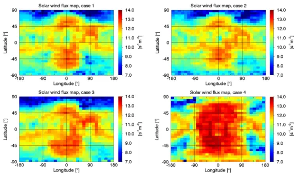
In Table 1 the interplanetary magnetic field (IMF) and solar wind conditions for four different cases used in the present simulations are summarized. Case 1 is intended to simulate ‘mean’ near-Mercury conditions similar to those measured during the first Mercury flyby (M1) of MESSENGER (Baker et al., 2009, 2011; Slavin et al., 2010), case 2 considers a northward directed IMF, and case 3 and case 4 represent solar wind conditions with a stronger IMF and higher solar wind density. Additionally, case 4 corresponds to a very high bulk speed. The calculated solar wind flux onto Mercury’s surface for all four cases is illustrated in Fig. 1.

2.2 Mercury’s surface composition

As outlined in Wurz et al. (2010) - besides disk-averaged spectra from the first MESSENGER flyby and spatially resolved observations from the Mercury

At-Fig. 1. Solar wind flux maps of precipitating H+ and He++ ions onto Mercury’s surface in units of s−1 m−2 for four different cases varying in the strength of the IMF, the solar wind bulk velocity vbulk, the solar wind density (H+ and He++ions)

nswand the helium fraction xHe(see Table 1). The subsolar point lies in the center of

the maps, positive latitudes correspond to Mercury’s northern hemisphere, positive longitudes represent the eastern hemisphere.

mospheric and Surface Composition Spectrometer (MASCS) instrument (Mc-Clintock et al., 2008) - the main knowledge of Mercury’s global average surface composition is mainly inferred from ground-based observations in the visible and IR spectral ranges, as well as from experiments with analogue materials in laboratories (Warell et al., 2006; Sprague et al., 2007, 2009; Wurz et al., 2010). However, ground-based measurements of Mercury’s surface mineralogy are hampered by various circumstances like the absorption features of the ter-restrial atmosphere in the infrared wavelength range or the planet’s closeness to the Sun. Furthermore, Mercury’s surface has experienced space weathering for more than 4 billion years (Hapke, 2001) resulting in a substantial regolith layer, which makes the spectroscopic identification of minerals on the surface

difficult.

Based on this available spectroscopic observations regarding the mineralog-ical information of Mercury’s surface, Wurz et al. (2010) designed a global mineralogical model of the planet’s elemental surface composition. This sur-face composition model consists of a selected group of end-member mineral compositions (∼ 27 mol% feldspar, ∼ 32 mol% pyroxene, ∼ 39 mol% olivine, ∼ 0.07 mol% metallic iron and nickel, ∼ 1.03 mol% sulphides, ∼ 0.07 mol% ilmenite, ∼ 1.45 mol% apatite), which are weighted to be consistent with the available observational constraints and yields an average surface density of ∼ 3.11 g cm−3_{. From this mineralogical model Wurz et al. (2010) obtained the}

elemental composition of Mercury’s surface by applying additive and multi-plicative surface composition modeling techniques. Additionally they applied the multiplicative model with an assumed invariant Ca fraction of 1.67 % to better reproduce ground-based Ca exosphere observations (Bida et al., 2000).

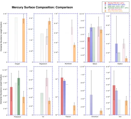
The elemental fractions given in Wurz et al. (2010) have been converted to weight fractions to allow comparison with the published data from the MES-SENGER mission, (Nittler et al., 2011; Rhodes et al., 2011; Peplowski et al., 2011, 2012; Starr et al., 2012; Weider et al., 2012). As can be seen from Fig. 2, the predicted abundances of most of the elements compare pretty well with the observations, which are O, Mg, Si, K, and Fe. For some elements like Ti and Cr, only upper limits are quoted from the measurements, which are com-patible with the predictions by the model. For Ca and Al the model predicted somewhat lower values. The measurements are not global averages, but for restricted areas on the surface, and show some local variation. For example, Peplowski et al. (2012) find that the average K abundance is 1150 and 1280 ppm for the areas sampled in 2011 and 2012, respectively. However, for

in-Fig. 2. Comparison of several measurements of the elemental surface compositions together with the predicted composition.

dividual locations the range of K abundances is between 754 and 1786 ppm. Similarly, Weider et al. (2012) find a range of abundances for many elements varying over a decade, depending on location on the surface. Considering the scatter between different measurements and the limited surface coverage, the agreement between the global abundances from Wurz et al. (2010) and the measurements is satisfactory (cf. Fig. 2).

In the present study we used the elemental surface composition derived from the multiplicative model with fixed Ca fraction of 1.67% from Wurz et al. (2010). The fractions are summarized in Table 2.

Table 2

Elemental surface abundance in units of atom percent as modeled with the mul-tiplicative composition modeling technique with a fixed Ca fraction of 1.67 % by Wurz et al. (2010). Species O Na Mg Al Si P S Abundance [%] 59.42 1.32 15.8 2.62 17.3 0.268 0.591 Species K Ca Ti Cr Fe Ni Zn Abundance [%] 0.030 1.670 0.014 0.041 0.611 0.004 0.285 2.3 Sputter yields

The sputter yields were obtained by means of the 2013 version of the SRIM package (Ziegler et al., 1984; Ziegler, 2004; Ziegler et al., 2013). The calcula-tions were performed for the multiplicative surface composition model with a fixed Ca fraction of 1.67 % (Table 2) with a surface mass density of 3.11 g cm−3 (Wurz et al., 2010) and an incident angle of impacting solar wind ions of 45◦ (Wurz et al., 2007). The sputter yields were calculated for the main constituents of impacting solar wind ions, i.e., for H+ and He++ ions. The contributions of heavier solar wind ions to the flux of sputtered material are less than 1 % (Wurz et al., 2010) because these ion fluxes are very low (Wurz, 2005), thus they were neglected. The total sputter yield Yi of species i was

calculated by: Yi = xHYiH+ xHeYiHe, where xH and xHe are the fractions of H+

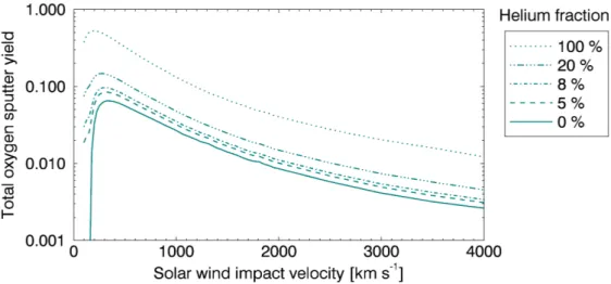
and He++ions in the solar wind, respectively, and Y_iHand Y_iHeare the sputter yields of species i caused by H+ and He++ ions respectively. Fig. 3 illustrates the total oxygen sputter yields for various solar wind helium fractions in the range of the solar wind impact velocity from 100 to 4000 km s−1. Helium

Fig. 3. Total oxygen sputter yields for different solar wind helium fractions.

sputtering is about 8 times more effective than proton-sputtering, thus for a typical solar wind helium fraction of 5%, about 30% of the total sputter yield is caused by helium sputtering. This fraction increases to 40% for a solar wind helium fraction of 8% and to 70% for a solar wind He fraction of 20%. The maximum sputter yield caused by He++ ions is about 0.53 oxygen atoms per impacting helium ion at an impact velocity of about 200 km s−1, whereas pro-tons produce at most 0.065 sputtered oxygen atoms per impacting proton at an impact velocity of about 320 km s−1. For lower impact velocities the sputter yields decrease rather strong, especially in the case of helium sputtering.

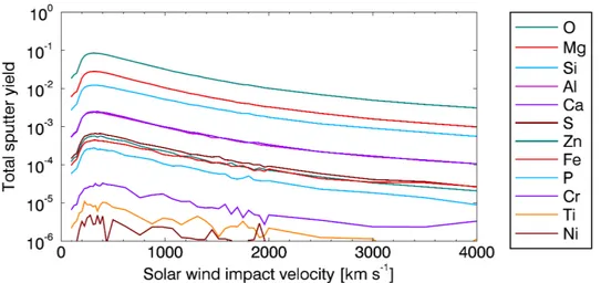
Fig. 4 gives an overview of the total sputter yields of 12 species (without K and Na) according to the multiplicative surface model with fixed Ca frac-tion of 1.67 % (Wurz et al., 2010). The total sputter yields cover a range of more then 4 magnitudes, resulting from the range of elemental abundances. Within a limited abundance range there is a linear relation between the total sputter yields and the elemental atomic surface fraction: Yi = YirelCi (Wurz

et al., 2007), which can be used for surface compositions very similar to the composition assumed used to obtain the total sputter yields.

Fig. 4. Total sputter yields for 12 surface elements obtained by the multiplicative surface composition model with a fixed Ca fraction of 1.67% (Wurz et al., 2010).

Mercury’s resulting sputter flux Φsp_i of species i is obtained by:

Φsp_i (ϑ, ϕ) = Φsw(ϑ, ϕ) Yi (1 − por) , (1)

with Φsw_{(ϑ, ϕ) the solar wind flux (H}+ _{and He}++ _{ions) depending on latitude}

ϑ and longitude ϕ as illustrated in Fig. 1, Yi the total sputter yield of species

i for the surface composition given in Table 2, and por the porosity of the regolith surface which is assumed to be 0.3 (Cassidy and Johnson, 2005; Wurz et al., 2010) and effectively reduces the sputter yield with regard to that of solid grains by 30 %.

2.4 3D exosphere modeling

The sputter yield of 12 chemical elements (see Table 2, without K and Na) caused by solar wind sputtering is the basic source in the modeling of Mer-cury’s exosphere, which depends on latitude and longitude as described by the solar wind flux maps (see Fig. 1).

The production rate Q in units of s−1 of particles generated in a surface element is calculated by

Q =

Z

Φsp_i dA , (2)

where A is the area and Φsp_i (ϑ, ϕ) the corresponding sputter flux of the surface element, given by Eq. (1). We generate a total of about 4×106pseudo particles equally distributed over Mercury’s surface. With N the number of pseudo particles of the considered surface element the production rate Qp, assigned

to each pseudo particle, is given by

Qp =

Q

N . (3)

The energy distribution of the sputtered species is taken from Sigmund (1969) that was extended to account for the maximum energy which can be imparted to a sputtered particle (Wurz and Lammer, 2003; Wurz et al., 2007):

f (Ee) = 6Eb 3 − 8qEb/Ec Ee (Ee+ Eb) 3 1 − s Ee+ Eb Ec ! (4) with Ec= Ei 4m1m2 (m1+ m2)2 , (5)

where Ee and Eb are the kinetic energy and the surface binding energy of

the sputtered particle with mass m2, respectively, and Ei is the energy of the

impacting particle m1. The distribution of the angle θ between the surface

normal and the initial trajectory of the sputtered particle is assumed to follow the Knudsen cosine law (Cassidy and Johnson, 2005):

f (β) ∝ cos θ. (6)

In the horizontal plane the velocity vector is assumed to be distributed uni-formly. Thus, we know the initial position and velocity vectors and the produc-tion rates of all pseudo particles. We divide the spherical space from Mercury’s

surface up to an altitude of 50 000 km into volume cells with a resolution of 200 km vertical, significantly less than the typical scale heights for sputtered species (hO = 1600 km, hMg = 1300 km, and hCa = 890 km, Wurz et al.

(2010)), and 6◦ in latitude and longitude, respectively. The trajectories of the pseudo particles are calculated by means of a second order Runge-Kutta in-tegration routine and the time t that the pseudo particle needs to transverse each cell is determined. The contribution of this pseudo particle to the num-ber of particles Npart inside the cells is then given by Npart = Qpt, and finally

the number density n in the considered cell is obtained by summing up the contributions from all pseudo particles and relating it to the cell volume Vc:

n =

P

Npart

Vc

. (7)

The integration of the particle trajectories is performed up to a distance of 50 000 km which is well within Mercury’s sphere of influence so that the grav-itational perturbation of the Sun can be neglected. The integration is termi-nated either when the particle exceeds this distance or when it falls back onto the surface, where we assume perfect sticking.

Depending on Mercury’s radial velocity with respect to the Sun, which is a function of it’s orbital position, the effect of solar radiation acceleration cannot be neglected for the elements Sodium, Potassium and Calcium (Smyth and Marconi, 1995; Potter et al., 2007; Potter and Killen, 2008; McClintock et al., 2009). Also Magnesium experiences this effect, but it is a factor of 4.7 × 10−3 weaker than Mercury’s surface gravity (McClintock et al., 2009) and will be neglected in this paper. Resonance scattering of solar radiation causes an

Table 3

Photionization rates in 10−6 s−1 for the quiet and active Sun at 1 AU, taken from Huebner et al. (1992)

.

Species O Mg Al Si P S Ca Ti Cr Fe Ni Zn quiet Sun 0.7 0.7 1200 23.2 0.6 1.1 69.6 2.5 3.8 1.8 0.9 0.5 active Sun 1.8 1.1 1300 48.5 1.4 2.3 78.0 5.7 8.9 3.7 1.9 1.4

acceleration a of the considered species

a = πhe 2_ν memc2 πFν f R2; (8)

here, m is the mass of the species, e and me denote charge and mass of an

electron, h is the Planck constant, ν is the frequency and f the oscillator strength of the resonance transition, (πFν) is the solar flux at 1 AU in the rest

frame of the species and R the heliocentric distance in AU.

Photoionization rates are taken from Huebner et al. (1992), and the online tool available at http://phidrates.space.swri.edu/ for both, the quiet and the active Sun and are listed in Table 4. The loss due to photoionization is taken into account by continously reducing the production rate Qp, assigned to the

considered pseudo particle, along its trajectory by the appropriate factor.

Finally the pseudo particles are considered to be lost if they exceed the maxi-mum altitude of 50 000 km, or if they impact on the surface. At this maximaxi-mum altitude more the 99 % of the particles have velocities exceeding the escape velocity, which justifies these particles to be treated as lost.

3 Results

We compare the results for the typical case 1 of all sputtered elements. Mer-cury’s heliocentric distance was chosen in accordance to MESSENGER’s first flyby (M1) as 0.35 AU corresponding to a true anomaly angle (TAA) of 285◦ (Vervack et al., 2010).

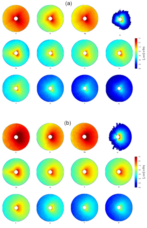
Fig. 5a illustrates the modeled number density in a meridian section (the Sun is to the right) for various refractory elements. Because of its high surface abundance (see Tab. 2), the oxygen density in the exosphere is significantly larger than the density of the other elements. Although the model surface abundances of magnesium and silicon are similar, the magnesium density is enhanced with respect to silicon because it can be released easier due to its lower surface binding energy of 1.54 eV compared to the Si binding energy of 4.7 eV. The density of aluminium rapidly falls off with increasing distance from the planet because its photoionization rate is much larger than that of the other elements (Table 4). Among the elements considered, solar radiation acceleration is only relevant for Ca, yielding to a Ca tail in the anti-sunward direction. It should be noted that the maximum density values obtained for the elements are somewhat higher than those given by Wurz et al. (2010) because the precipitation rates of solar wind ions is not uniform over the surface. Higher ion precipitation fluxes at localized regions can lead to higher exospheric densities at the surface than the average densities published by Wurz et al. (2010). Fig. 5b displays the 3-dimensional exosphere density for the extreme case 4. With respect to case 1, the densities are significantly increased because the solar wind can effectively sputter particles from the whole dayside surface of Mercury (compare Fig. 1).

Fig. 5. Meridian volume density plots with the Sun at the right side for (a) case 1 and (b) case 4 within 6 hermean radii (0 - 15000 km altitude) around the planet. Note that both figures display the same color scaling.

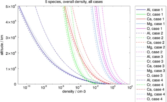
Fig. 6. Altitude density profiles of 5 selected species for all cases.

Fig. 6 shows altitude density profiles averaged over the entire planet of 5 selected species for all 4 cases to compare the differences between them. For all elements case 2 results in lower densities compared to case 1, whereas case 3 shows slightly enhances densities. Case 4 results in density enhancements of one to two orders of magnitude depending on the considered element and the altitude, although the corresponding sputter yields are about three times less than for case 1 (compare with Figs. 3 and 4).

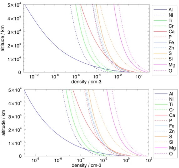
In Fig. 7a,b altitude density profiles averaged over the entire planet are shown for the cases 1 and 4 for all considered species. Al and Ca have lower scale heights than the other elements because of the high photoionization rate for Al and the radiation acceleration effect of Ca which reduces the scale height. Figs. 8a and b display the density profiles of several species for the cases 1 and 4 obtained by averaging the density separately over the day- and night-side. Nightside densities are always lower than the density at dayside with the

Fig. 7. Altitude density profiles of all considered species for case 1 (upper panel) and case 4 (lower panel).

exception of Ca, where the particles are transported into the nightside hemi-sphere due to the solar radiation acceleration. For case 1, at about 8000 km altitude, the nightside Ca-density exceeds the dayside Ca-density, while for case 4, the nightside density starts to exceed the dayside density at 50 000 km height. Figs. 8a,b also include the density profile of aluminium when photoion-ization is neglected (annotated by ”no pi”), showing that Al is diminished at higher altitudes due to photoionization by several orders of magnitude.

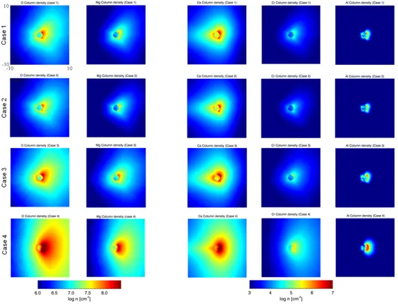
Fig. 9 displays column densities of selected elements obtained by integrating along a line parallel to the Sun-planet line at 10 planetary radii and looking

Fig. 8. Day/nightside profiles for case 1 (upper panel) and case 4 (lower panel). For Al both profiles with and without (no pi) photionization are shown.

towards the noon-midnight plane of the planet. The density integrated along the line of sight is projected onto the plane defined by Mercury’s north pole and the Sun-Mercury line. The four rows correspond to the cases 1–4. Note the different scaling of O and Mg with respect to the other elements. While the column densities are quite similar for case 1 and 2, the calculated column densities increase with increased IMF and solar wind density (case 3) and become significantly larger for the high solar wind bulk velocity (case 4). In the latter case, the entire dayside surface of the planet experiences intense ion sputtering which results in column densities enhanced by more than one order of magnitude with respect to the nominal conditions of case 1. Due to the effective photoionization, even in the extreme case 4 higher Al densities

Fig. 9. Column densities for the cases 1 to 4 obtained by projecting the density integrated along the line of sight onto the plane defined by Mercury’s north pole and the Sun-Mercury line.

are expected only in a relatively small volume above the dayside of Mercury, while the nightside remains almost uneffected by the stronger solar wind.

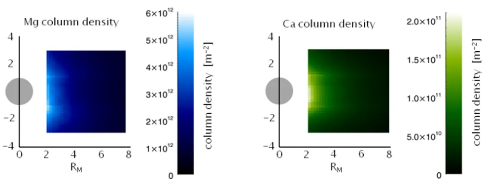
Although the magnetic field configuration was different for M1 and M2, the orbital parameters of Mercury and the radiation acceleration were quite similar (Vervack et al., 2010), suggesting comparable column densities during M1 and M2. Fig. 10 illustrates the simulated column densities of Mg and Ca for case 1 (corresponding to M1 conditions) in the nightside of Mercury by using a linear color scale to allow a better comparison with MESSENGER tail observations, where radiance maps of Mg and Ca were recorded as the spacecraft approached the planet (McClintock et al., 2009). Reported column emissions for Mg and Ca cover a range between 0–250 and 0–600 Rayleighs, respectively, during the

Fig. 10. Column densities of Mg and Ca for case 1 projected onto the plane defined by Mercury’s north pole and the Sun-Mercury line.

second flyby. Using the published g-values of g = 0.318 for Mg and g = 22.07 for Ca (Vervack et al., 2010), this corresponds to a column density range of approximately 0–8 · 1012 _{and 0–3 · 10}11 _m−2 _{and is in reasonable agreement}

with the simulation results displayed in Fig. 10.

The impact rates of sputtered particles falling back on the surface of Mercury and the esacpe rates of exospheric particles are listed in Table 5 for the four cases considered. For oxygen, the escape rates distinctly exceed the impact rates, because the sputter distribution, eq. (4), peaks close to the escape energy so that a considerable amount of sputtered oxygen atoms will acquire velocities above the escape velocity. For the other species, however, the distribution function peaks at lower energies than the escape energy, leading to an increased generation of particles along bound orbits, which eventually fall back onto the surface. Over a long period, the large variation of the escape rates of different species may result in a distinct fractionation of the surface composition, in particular suggesting a strong depletion of the oxygen content of the surface.

Table 4

Impact and escape rates

species Case 1 Case 2 Case 3 Case 4

impact escape impact escape impact escape impact escape [s−1] [s−1] [s−1] [s−1] [s−1] [s−1] [s−1] [s−1] O 4.9 · 1023 _{2.0 · 10}24 _{3.4 · 10}23 _{1.4 · 10}24 _{8.6 · 10}23 _{3.4 · 10}24 _{2.2 · 10}24 _{1.0 · 10}25 Si 6.5 · 1022 _{5.4 · 10}22 _{4.5 · 10}22 _{3.7 · 10}22 _{1.2 · 10}23 _{9.0 · 10}22 _{3.3 · 10}23 _{3.9 · 10}23 Mg 2.6 · 1023 _{5.6 · 10}23 _{1.8 · 10}23 _{3.9 · 10}23 _{4.6 · 10}23 _{9.4 · 10}23 _{1.2 · 10}24 _{2.9 · 10}24 Al 6.7 · 1019 _{3.5 · 10}16 _{4.7 · 10}19 _{2.6 · 10}16 _{1.2 · 10}20 _{3.4 · 10}16 _{3.1 · 10}20 _{4.4 · 10}18 Ca 1.1 · 1022 _{1.2 · 10}21 _{7.6 · 10}21 _{8.7 · 10}20 _{1.9 · 10}22 _{2.1 · 10}21 _{5.7 · 10}22 _{1.0 · 10}22 Fe 8.0 · 1021 _{4.2 · 10}21 _{5.6 · 10}21 _{2.9 · 10}21 _{1.4 · 10}22 _{6.8 · 10}21 _{4.4 · 10}22 _{3.3 · 10}22 S 8.1 · 1021 1.1 · 1022 5.6 · 1021 7.7 · 1021 1.4 · 1022 1.8 · 1022 3.8 · 1022 6.5 · 1022 Zn 1.2 · 1022 _{5.0 · 10}21 _{8.4 · 10}21 _{3.5 · 10}21 _{2.0 · 10}22 _{7.5 · 10}21 _{5.4 · 10}22 _{3.5 · 10}22 P 3.2 · 1021 _{4.6 · 10}21 _{2.2 · 10}21 _{3.2 · 10}21 _{5.5 · 10}21 _{7.6 · 10}21 _{1.6 · 10}22 _{2.9 · 10}22 Cr 5.5 · 1020 _{2.9 · 10}20 _{3.8 · 10}20 _{2.0 · 10}20 _{8.6 · 10}20 _{4.2 · 10}20 _{2.7 · 10}21 _{2.0 · 10}21 Ti 1.7 · 1020 _{1.1 · 10}20 _{1.2 · 10}20 _{7.9 · 10}19 _{1.9 · 10}20 _{1.3 · 10}20 _{7.7 · 10}20 _{7.1 · 10}20 Ni 5.4 · 1019 _{2.7 · 10}19 _{3.8 · 10}19 _{1.9 · 10}19 _{1.6 · 10}20 _{6.9 · 10}19 _{3.6 · 10}20 _{2.6 · 10}20 4 Summary and Conclusion

A 3D hybrid solar wind interaction model has been applied to a global miner-alogical surface composition model of Mercury. The resulting sputtered refrac-tory elements and their release into the planet’s exosphere, the corresponding density distributions from the surface up to 50 000 kilometers and the escape rates have been simulated for various solar wind conditions. It is shown that the exosphere density of O, Mg, Al, Si, P, S, Ca, Ti, Cr, Fe, Ni, and Zn, com-pared to quiet or moderate solar wind conditions, can be enhanced by more than one order of magnitude during fast and denser solar wind events, where Mercury’s magnetosphere is so compressed by the plasma ram pressure that H+ and He++ ions can precipitate onto the planet’s surface over the whole dayside. Our results are also in agreement with MESSENGER observations of exospheric Ca and Mg particles. Less abundant refractory elements, which are difficult to observe during nominal solar wind conditions, may become

temporarily detectable when the planet is hit by a fast and dense plasma cloud.

References

Anderson, B.J., Johnson, C.L., Korth, H., Purucker, M.E., Winslow, R.M., Slavin, J.A., Solomon, S.C., McNutt Jr., R.L., Raines, J.M., Zurbuchen, T.H., 2011. The global magnetic field of Mercury from MESSENGER orbital observations. Science 333, 1859–1862.

Baker, D.N., Odstrcil, D., Anderson, B.J., Arge, C.N., Benna, M., Gloeck-ler, G., Korth, H., Mayer, L.R., Raines, J.M., Schriver, D., Slavin, J.A., Solomon, S.C., Tr´avn´ıˇcek, P.M., Zurbuchen, T.H., 2011. The space envi-ronment of Mercury at the times of the second and third messenger flybys. Planetary and Space Science 59, 2066–2074.

Baker, D.N., Odstrcil, D., Anderson, B.J., Arge, C.N., Benna, M., Gloeckler, G., Raines, J.M., Schriver, D., Slavin, J.A., Solomon, S.C., Killen, R.M., Zurbuchen, T.H., 2009. Space environment of Mercury at the time of the first messenger flyby: solar wind and interplanetary magnetic field modeling of upstream conditions. Journal of Geophysical Research 114, ?–?

Bida, T.A., Killen, R.M., Morgan, T.H., 2000. Discovery of calcium in Mer-cury’s atmosphere. Nature 404, 159–161.

Cassidy, T., Johnson, R., 2005. Monte Carlo model of sputtering and other ejection processes within a regolith. Icarus 176, 499–507.

Evans, L.G., Peplowski, P.N., Rhodes, E.A., Lawrence, D.J., McCoy, T.J., Nit-tler, L.R., Solomon, S., Sprague, A.L., Stockstill-Cahill, K.R., Starr, R.D., Weider, S.Z., Boynton, W.V., Hamara, D.K., Goldsten, J.O., 2012. Major-element abundances on the surface of mercury: Results from the messenger

gamma-ray spectrometer. Journal of Geophysical Research 117, E00L07. doi:10.1029/2012JE004178.

Hapke, B., 2001. Space weathering from Mercury to the asteroid belt. Journal of Geophysical Research 106, 10039–10074.

Huebner, W.F., Keady, J.J., Lyon, S.P., 1992. Solar photo rates for planetary atmospheres and atmospheric pollutants. Astrophysics and Space Science 195, 1–294. doi:10.1007/BF00644558.

Johnson, C.L., Purucker, M.E., Korth, H., Anderson, B.J., Winslow, R.M., Al Asad, M.M.H., Slavin, J.A., Alexeev, I.I., Phillips, R.J., Zuber, M.T., Solomon, S.C., 2012. MESSENGER observations of Mercurys magnetic field structure. Journal of Geophysical Research 117. doi:10.1029/2012JE004217. Kallio, E., Janhunen, P., 2003a. Modelling the solar wind interaction with Mercury by a quasi-neutral hybrid model. Annales Geophysicae 21, 2133– 2145. doi:10.5194/angeo-21-2133-2003.

Kallio, E., Janhunen, P., 2003b. Solar wind and magnetospheric ion im-pact on Mercury’s surface. Geophysical Research Letters 30, 1877. doi:10.1029/2003GL017842.

Kallio, E., Janhunen, P., 2004. The response of the Hermean magnetosphere to the interplanetary magnetic field. Advances in Space research 33, 2176– 2181. doi:10.1016/S0273-1177(03)00447-2.

Killen, R., Cremonese, G., Lammer, H., Orsini, S., Potter, A.E., Sprague, A.L., Wurz, P., Khodachenko, M.L., Lichtenegger, H.I.M., Milillo, A., Mura, A., 2007. Processes that promote and deplete the exosphere of Mercury. Space Science Reviews 132, 433–509. doi:10.1007/s11214-007-9232-0.

McClintock, W.E., Izenberg, N.R., Holsclaw, G.M., Blewett, D.T., Domingue, D.L., Head, J.W., Helbert, J., McCoy, T.J., Murchie, S.L., Robinson, M.S., Solomon, S.C., Sprague, A.L., Vilas, F., 2008. Spectroscopic Observations of

Mercury’s Surface Reflectance During MESSENGER’s First Mercury Flyby. Science 321, 62–65. doi:10.1126/science.1159933.

McClintock, W.E., Vervack, R.J., Bradley, E.T., Killen, R.M., Mouawad, N., Sprague, A.L., Burger, M.H., Solomon, S.C., Izenberg, N.R., 2009. MES-SENGER observations of Mercury’s exosphere: Detection of magnesium and distribution of constituents. Science 324, 610.

Nittler, L.R., Starr, R.D., Weider, S.Z., McCoy, T.J., Boynton, W.V., Ebel, D.S., Ernst, C.M., Evans, L.G., Goldsten, J.O., Hamara, D.K., Lawrence, D.J., McNutt, R.L., Schlemm, C.E., Solomon, S.C., Sprague, A.L., 2011. The Major-Element Composition of Mercury’s Surface from MESSENGER X-ray Spectrometry. Science 333, 1847–1850.

Peplowski, P.N., Evans, L.G., Hauck, S.A., McCoy, T.J., Boynton, W.V., Gillis-Davis, J.J., Ebel, D.S., Goldsten, J.O., Hamara, D.K., Lawrence, D.J., McNutt, R.L., Nittler, L.R., Solomon, S.C., Rhodes, E.A., Sprague, A.L., Starr, R.D., Stockstill-Cahill, K.R., 2011. Radioactive Elements on Mer-curys Surface from MESSENGER: Implications for the Planets Formation and Evolution. Science 333, 1850–1852.

Peplowski, P.N., Lawrence, D.J., Rhodes, E.A., Sprague, A.L., McCoy, T.J., Denevi, B.W., Evans, L.G., Head, J.W., Nittler, L.R., Solomon, S.C., Stockstill-Cahill, K.R., Weider, S.Z., 2012. Variations in the abundances of potassium and thorium on the surface of Mercury: Results from the MES-SENGER Gamma-Ray Spectrometer. Journal of Geophysical Research: Planets 117. doi:10.1029/2012JE004141.

Potter, A.E., Killen, R.M., 2008. Observations of the sodium tail of Mercury. Icarus 194, 1–12. doi:10.1016/j.icarus.2007.09.023.

Potter, A.E., Killen, R.M., Morgan, T.H., 2007. Solar radiation ac-celeration effects on Mercury sodium emission. Icarus 186, 571–580.

doi:10.1016/j.icarus.2006.09.025.

Rhodes, E.A., Evans, L.G., Nittler, L.R., Starr, R.D., Sprague, A.L., Lawrence, D.J., McCoy, T.J., Stockstill-Cahill, K.R., Goldsten, J.O., Peplowski, P.N., Hamara, D.K., Boynton, W.V., Solomon, S.C., 2011. Analysis of MESSEN-GER Gamma-Ray Spectrometer data from the Mercury flybys. Planetary and Space Science 59, 1829–1841.

Sigmund, P., 1969. Theory of sputtering. I. sputtering yield of amor-phous and polycrystalline targets. Physical Review 184, 383–416. doi:10.1103/PhysRev.184.383.

Slavin, J.A., Lepping, R.P., Wu, C.C., Anderson, B.J., Baker, D.N., Benna, M., Boardsen, S.A., Killen, R.M., Korth, H., Krimigis, S.M., et al., 2010. MESSENGER observations of large flux transfer events at Mercury. Geo-physical Research Letters 37, L02105.

Smyth, W.H., Marconi, M.L., 1995. Theoretical overview and modeling of the sodium and potassium atmospheres of Mercury. The Astrophysical Journal 441, 839–864. doi:10.1086/175407.

Sprague, A., Warell, J., Cremonese, G., Langevin, Y., Helbert, J., Wurz, P., Veselovsky, I., Orsinis, S., Milillo, A., 2007. Mercury’s surface composition and character as measured by ground-based observations. Space Science Reviews 132, 399–431.

Sprague, A.L., Donaldson Hanna, K.L., Kozlowsky, R.W.H., Helbert, J., Ma-turilli, A., Warell, J.B., Hora, J.L., 2009. Spectral emissivity measurements of Mercury’s surface indicate Mg- and Ca-rich mineralogy, K-spar, Na-rich plagioclase, rutile, with possible perovskite, and garnet. Planetary and Space Science 57, 364–383.

Starr, R.D., Schriver, D., Nittler, L.R., Weider, S.Z., Byrne, P.K., Ho, G.C., Rhodes, E.A., Schlemm, C.E., Solomon, S.C., Tr´avn´ıˇcek, P.M.,

2012. MESSENGER detection of electron-induced X-ray fluorescence from Mercurys surface. Journal Geophysical Research 117, 1–19. doi:10.1029/2012JE004118.

Vervack, R.J., McClintock, W.E., Killen, R.M., Sprague, A.L., Anderson, B.J., Burger, M.H., Bradley, E.T., Mouawad, N., Solomon, S.C., Izenberg, N.R., 2010. Mercury’s complex exosphere: Results from MESSENGER’s third flyby. Science 329, 672.

Warell, J., Sprague, A.L., Emery, J.P., Kozlowsky, R.W.H., Long, A., 2006. The 0.7-5.3 µm IR spectra of Mercury and the Moon: Evidence for high-Ca clinopyroxene on Mercury. Icarus 180, 281–291.

Weider, S.Z., Nittler, L.R., Starr, R.D., McCoy, T.J., Stockstill-Cahill, K.R., Byrne, P.K., Denevi, B.W., Head, J.W., Solomon, S.C., 2012. Chemical heterogeneity on Mercury’s surface revealed by the MESSENGER X-Ray Spectrometer. Journal of Geophysical Research: Planets 117.

Wurz, P., 2005. Solarwind composition, in: The Dynamic Sun: Challenges for Theory and Observations, ESA. pp. 1–9. doi:2005ESASP.600E..44W. Wurz, P., Lammer, H., 2003. Monte-Carlo simulation of Mercury’s exosphere.

Icarus 164, 1–13. doi:16/S0019-1035(03)00123-4.

Wurz, P., Rohner, U., Whitby, J.A., Kolb, C., Lammer, H., Dobnikar, P., Mart´ın-Fern´andez, J.A., 2007. The lunar exosphere: The sputtering contri-bution. Icarus 191, 486–496.

Wurz, P., Whitby, J.A., Rohner, U., Mart´ın-Fern´andez, J.A., Lammer, H., Kolb, C., 2010. Self-consistent modelling of Mercury’s exosphere by sputter-ing, micro-meteorite impact and photon-stimulated desorption. Planetary and Space Science 58, 1599–1616. doi:16/j.pss.2010.08.003.

Ziegler, J.F., 2004. SRIM-2003. Nuclear Instruments and Methods in Physics Research Section B: Beam Interactions with Materials and Atoms 219-220,

1027–1036. doi:10.1016/j.nimb.2004.01.208.

Ziegler, J.F., Biersack, J.P., Littmark, U., 1984. The Stopping and Range of Ions in Solids. volume 1 of Stopping and Ranges of Ions in Matter. Pergamon Press, New York.

Ziegler, J.F., Biersack, J.P., Ziegler, M.D., 2013. www.srim.org. URL checked on 2014/01/13.