ALMA MATER STUDIORUM
UNIVERSITA' DI BOLOGNA
SCUOLA DI SCIENZE
Corso di laurea magistrale in Biologia Marina
HABITAT USE OF MIGRATING DWARF MINKE WHALES (Balaenoptera
acutorostrata subspecies) IN TASMANIAN WATERS
Tesi di laurea in
Disegni Sperimentali e Analisi Dati
Relatore
Presentata da
Prof. Marina A. Colangelo
Elena Fontanesi
Correlatore
Prof. Mary-Anne Lea
Prof. Mark Hindell
Prof. Russel Andrews
III sessione
1 Table of contents
1. Preface………... 3
2. Literature review………... 4
2.1 Introduction………. 4
2.2 The study of cetacean distribution and habitats... 5
Brief description of cetaceans... 5
Collecting data on cetacean distribution... 6
Collecting habitat data... 8
Modelling cetacean distribution... 10
2.3 Baleen whales in Australian waters... 12
Humpback whale... 12
Pigmy blue whale... 13
Southern right whale... 15
2.4 Dwarf minke whale... 17
Taxonomy... 17 Distribution... 18 Abundance... 19 Biology... 20 2.5 Current study... 20 Chosen methods... 20 3. Scientific paper... 22 Abstract... 22
2
3.1 Introduction... 23
3.2 Materials and methods... 25
Tag deployment... 25
Tracking data processing... 26
Data analysis... 26 Time-spent analysis... 27 Environmental data... 27 Statistical modelling... 29 Regional comparisons... 30 3.3 Results... 31
Dwarf minke whales movements... 32
Time-spent analysis... 33
Statistical modelling... 34
Regional comparisons... 36
3.4 Discussion... 37
Dwarf minke whales habitat use in relation to environmental covariates... 37
Biological relevance of high time-spent areas... 39
Implications for management... 41
Future directions... 42
4. Literature cited... 43
3 1. Preface
This work is the result of my exchange study period at the University of Tasmania, Australia. I spent a semester working at the Institute of Marine and Antarctic Studies supervised by Dr. Mary-Anne Lea, Dr. Mark Hindell, Dr. Russel D. Andrews and followed by email by Prof. Marina A. Colangelo on the first tracking data available for dwarf minke whales (Balaenoptera acutorostrata subspecies). These data were collected thanks to the collaboration of Dr. Russel D. Andrews, Dr. R. Alastair Birtles, Dr. Jimmy White, K. Curt. N. Jenner, and John Rumney and several institutions and funding programs, mentioned in the acknowledgements.
This work is divided in two main parts, according to the project’s development. First, a literature review aiming to give background information on whales around Australia, technologies adopted to study whales’ migrations, modelling frameworks to infer organism’s habitat use and preference related to environmental characteristics. The literature review consisted in a revision of papers available on the topic, and it was of essential importance in the further choice of the best methodologies to deal with my research questions.
The second part is the outcome of the actual work with the tracking data and shows the methods used, the results obtained and the following discussions. I decided to split the contents of the main chapters in smaller sections to allow an easier understanding of the steps undertook.
4 2. Literature review
2.1 Introduction
Krausman (1999) defined habitat as ‘the resources and conditions present in an area that produce occupancy, including survival and reproduction, by a given organism.’ For this reason, habitat is species-specific and includes migration and dispersal corridors as well as areas were the animal feed and breed. Understanding animals distribution and the processes that drive their habitat selection, is of crucial importance for the management and protection of species (Redfern et al. 2006). This is becoming increasingly urgent as the combination of climate change and anthropogenic activities are threatening the existence of many ecosystems as we know them today, with possible implications on species’ wellness.
Marine ecosystems are known to be naturally very dynamic and fluid, with variability operating on diurnal to decadal scales and from meters to 1000s kilometres (Redfern et al. 2006). Long-living, wide-ranging animals such as cetaceans may respond to this variability by changing their distribution patterns (Forney 2000) to avoid changes in survival and reproductive success. Nevertheless, these are unavoidable consequences if new suitable areas with similar characteristics cannot be found. For this reason many studies on cetaceans are addressing the task of understanding their distribution by linking their presence to different environmental variables (Panigada et al. 2008).This is driven by the aim of discerning which habitats are suitable, and subsequently need to be preserved, for each species (Hooker et al. 1999, Bruce et al. 2014).
The methodologies adopted in the collection of data for these kind of studies are quite diverse. They include boat surveys (Panigada et al. 2008), aerial surveys (Gales et al. 2012), acoustic tracking (Mathias et al. 2013) and satellite telemetry (Andrews et al. 2008). Satellite telemetry in particular, is becoming increasingly employed by scientists, predominantly due to technological improvements and its progression in becoming more financially accessible. Environmental and oceanographic data to correlate with animal distribution can either be collected on site or derived from satellite data (Redfern et al. 2006) and are essential to develop explanatory or predictive habitat models.
Many species of baleen whales are known to migrate seasonally from wintering high latitude foraging grounds, to summering tropical mating and breeding grounds (De Sá Alves et al. 2009). Migration routes have been regarded solely as corridors crossed by animals to reach
5
the two most important areas. However, the importance of these routes is being re-evaluated due to the emergence of opportunistic feeding records (Stamation et al. 2007) and longer permanence in some locations where resting behaviours have been documented (Bruce et al. 2014).
Australia is an important feeding, breeding and resting ground or migrating corridor for different baleen whales, including populations of humpback whales (Corkeron et al. 1994), pigmy right whales (Kemper et al. 2013), blue whales (Gill et al. 2011) and dwarf minke whales (Birtles et al. 2002). While the knowledge on some of these species’ life histories is quite detailed, the migration of dwarf minke whales that breed in the Great Barrier Reef is still unknown (Sobtzick 2010). This needs to be investigated to better manage these marine mammals.
This review will explore the current state of knowledge on migrating whales around Australia; the methodologies used to comprehend their movements and their use of various habitats. The ultimate aim of the research is to generate a better understanding of the species’ ecology, as well as provide information to assist in the improved management and protection of migrating whales. It will start with a basic description on cetaceans and examine different approaches employed to study these animals and their relationship with the environment. This will include an examination of which factors determine their distribution and could be employed to provide a sufficient habitat-model. It will then focus on baleen whale populations that use Australian waters during various stages of their life histories, highlighting the missing knowledge for some of them, as the one focus of my study: dwarf minke whales.
2.2 The study of cetacean distribution and habitats Brief description of cetaceans
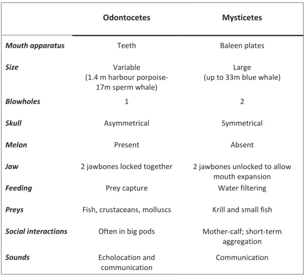
Cetaceans are, with sirenians, the only mammals that spend their entire life cycle in the water, as predisposed by their unique anatomical and physiological adaptations to the marine environment (Jefferson et al. 2011). The infraorder Cetacea currently includes 93 species of dolphins, whales and porpoises inhabiting oceans, lakes and rivers (Perrin 2009). It comprises the superfamily Misticetes, also known as baleen whales and the superfamily Odontocetes or toothed whales. The main difference between the two is the foraging strategies due to their dissimilar mouth apparatus: baleen whales have baleen plates to filter water and feed mainly
6
on krill and small fish, while dolphins and toothed whales use their homodont teeth to forage on fish, molluscs and crustaceans. Apart from great differences in size and anatomy, they have also diverse behaviours, life histories and social structures (Table 1).
Odontocetes Mysticetes
Mouth apparatus Teeth Baleen plates
Size Variable
(1.4 m harbour porpoise- 17m sperm whale)
Large
(up to 33m blue whale)
Blowholes 1 2
Skull Asymmetrical Symmetrical
Melon Present Absent
Jaw 2 jawbones locked together 2 jawbones unlocked to allow mouth expansion
Feeding Prey capture Water filtering
Preys Fish, crustaceans, molluscs Krill and small fish
Social interactions Often in big pods Mother-calf; short-term aggregation
Sounds Echolocation and
communication
Communication
Table 1: main differences between Odontocetes and Mysticetes, adapted from Birds and Mammals of the Southern Ocean lecture material, Mary-Anne Lea.
Collecting data on cetacean distribution
Conducting research on cetaceans presents many difficulties due to both the environment they live in and their behaviours. Being highly mobile and spending the majority of time underwater, detecting them and accurately estimating the group size can be quite demanding (Redfern et al. 2006). Scientists have developed various techniques of collecting data on cetacean distribution and environmental features. These have predominantly been developed through adapting methodologies used with other animals, to suit these particular mammals and environments.
7
There are several approaches that can be adopted in the collection of data about marine mammals’ distribution, the selection of which method to employ depends mainly on the study question, the species and the available funding. These include ship, aerial and acoustic surveys, tagging studies as well as opportunistic data.
Ship and aerial visual surveys with dedicated platforms can provide useful estimates of cetacean distribution, even if they often impose limitations on spatial and temporal extent because of the high costs (Evans & Hammond 2004). These surveys are based on linear transect sampling methods (Buckland et al. 2001), generated through the extrapolation of species density in the study area, from the number of animals counted in a series of transects. For this reason, the transects need to be designed to allow for the entire study area to have the same probability of being sampled (Redfern et al. 2006). Common sampling designs consist of a series of parallel and equally spaced lines or zigzag patterns (Figure 1), starting from a random point of the survey area borders (Evans & Hammond 2004).
Usually, the actual realisation of these transects is likely to be compromised by logistical problems such as the weather and mechanical difficulties (Redfern et al. 2006).The use of aircrafts might be more effective in the detection of animals, however prevents the collection of local environmental data. In these types of surveys, there is a possibility for perception bias where animals may not be counted even if present, due to either animal behaviours and group size or survey conditions such as sea state, swell, visibility, and availability bias where the animals are not detected because they are submerged (Marsh & Sinclair 1989).
Acoustical surveys are less expensive than visual ones, but at the moment do not provide a quantitative estimation on animal density because it is still unknown whether vocalisation varies within different age, gender, single individuals and seasons (Redfern et al. 2006). Barlow and Taylor (2005) used acoustic methods as well as visual sampling to detect the presence of sperm whales during ship surveys. They concluded that the use of towed hydrophone arrays increased the number of animals detected and allowed night-time surveys, but at the same time a combination of the two methodologies was needed to assess the group size. Besides the clear limitations of acoustic surveys, they can provide information about species habitat use or migration on large spatial and temporal scales.
Tagging studies can provide information on long distance movements as well as on fine-scale data on behaviour, physiology and ecology (Costa 1993). Rapid technology developments in recent years have led to a variety of different bio-logging devices with increased capabilities.
8
From a first time-depth recorder lasting one hour used on Weddel seals in 1963, we now have satellite transmitters that can quite precisely identify the animals’ position, and can also be combined with camcorders to generate data on animal behaviour underwater (Kooyman 2004). Thanks to the possibility of accessing animals on shore to deploy the devices, these technologies have been extensively used on pinnipeds (Hindell et al. 1991, Bradshaw 2002, McMahon et al. 2008). These are also popular tools among cetacean researchers, despite the marine environment being more demanding than land-based tagging scenarios (Goldbogen et al. 2008, Gales et al. 2012, Vikingsson & Heide-Jorgensen 2015). Nowadays, tagging devices can also collect information on the environment, providing fine-scale habitat data (Roquet et al. 2013). Recording greater quantities of data requires greater-capacity batteries and consequently bigger tags, and this is likely to affect organisms’ wellness and fitness (Watkins & Tyack 1991). Due to financial and time constraints placed on tagging data collection techniques, the sample size is often quite small and extrapolation of results to a population level needs to be proceeded with caution (Redfern et al. 2006). Five main types of tags exist :very-high frequency (VHF), geolocation, acoustic, Argos and global positioning system (GPS). The selection of which tagging system to employ depends on species, research aims, temporal and spatial scales and consequently on how important size, memory, longevity and resolution are to the specific study (Green et al. 2009) . Photo-identification and focal follows are other types of tagging which are significantly less expensive and invasive, and can provide good data about animal distribution and migration patterns (Carlson et al. 1990) . Data on cetacean distribution can also be opportunistically collected. Many studies are performed on platforms of opportunity such as ferries, research vessels, merchant marine ship or fishing vessels providing a large amount of data at low cost (Kiszka et al. 2007). In this case, disadvantages are associated with the varying levels of observer experience and the distance animals are being observed at, which can cause bias on species identification and group size. Whaling records can provide information about past trends in large whale distribution. Redfern et al. (2006) argued that whaling record data must be treated with caution, as it is not possible to assess whether whales were absent in some areas or simply the fishing effort presided greater concentration in other areas.
Collecting habitat data
Understanding what drives cetacean distribution requires an in-depth knowledge of the characteristics associated with the habitat where they are detected. It is not always possible to
9
have a priori knowledge of which environmental covariates are important in creating a habitat suitable for a particular population in a particular area, and the same species might prefer different environments throughout the varying life stages. Usually, physical oceanographic data are used as proxies for prey distribution, which is likely to be the greatest determinant for animal distribution (Redfern et al. 2006). However, during mating and reproductive seasons, there may be other motivations not related to food presence which drive animals’ habitat choice.
Data on environmental parameters can be collected in situ during cetacean surveys. Commonly measured variables include: surface water conditions like salinity, temperature, fluorescence, chlorophyll-a, dissolved oxygen content, as well as water column properties like depth of thermocline, mixed layer and euphotic zone (D'Amico et al. 2003, Tynan et al. 2005). Interestingly, it is also possible to broadly describe the ecological community, for example during humpback whale sightings on the east coast of Tasmania, Gill et al. (1998) collected water samples from the water column by towing a net, in order to determine whether the whales were feeding and what prey they were targeting during their migration. Acoustic devices such as echo sounders can be another methodology to study prey density and distribution (Murase et al. 2002). Requiring substantial investments of resources, in situ data collection often results in limited or infrequent areas surveyed, but can provide very accurate measurements of water properties and oceanographic characteristics.
Some tagging devices are programmed to collect data on sea temperature and salinity, allowing researchers to derive in situ conditions directly from the animals (Roquet et al. 2013). It is important to note that the use of these data in the study of habitat preferences can be misleading, as no comparative data of unused areas are recorded (Redfern et al. 2006). In studies where the methodology does not permit the collection of environmental data, it is possible to derive this data from bathymetric datasets, remotely sensed data and oceanographic processes models. Bathymetry is often openly accessible with a variety of data available on numerous global locations. From this, it is possible to calculate other variables such as bottom slope, distance to shore and distance to shelf break that might be important in the evaluation of marine mammals’ distribution (Gill et al. 2011, Muelbert et al. 2013). Chlorophyll-a, sea surface temperature, sea surface height can be easily obtained from satellite-derived data. They can be used to infer the presence of upwelling (Gill et al. 2011), fronts (Baumgartner et al. 2001) and other oceanographic features that can enhance the
10
productivity or concentration of preys. The main disadvantage of remote sensed data, is that the spatial and temporal resolution might not be fine enough to be coupled with animal sightings. Moreover, areas with frequent cloud cover can lack data for several days or weeks and only averages on longer periods can be used (Redfern et al. 2006). Ocean circulation models can also be an important source of environmental data. Models that couple circulation to biological processes are also available, making it possible to interfere the distribution of nutrients and phytoplankton (Moore et al. 2001) or the transport of zooplankton and fish larvae (Carlotti et al. 2000).
Modelling cetacean distribution
Cetacean-habitat modelling aims to reveal the mechanisms that drive animal distribution and has the potential to be a very powerful tool for cetacean conservation and mitigation of anthropogenic impacts on both species and the environment. Modelling is a mathematical interpretation of the relationship within a response variable and some predictors and is becoming increasingly employed in cetacean studies. The response variable can be the presence/absence of animals or the time spent by animals in a particular area, so indications of animals distribution as obtained during surveys or from tagging devices. The predictors can be any oceanographic or habitat features that have some influences on animal distribution either collected in the field or derived from remote sensed data.
Not many are the cetacean species where a priori knowledge of the ecological processes affecting allocation patterns are present. Extensive knowledge of the main oceanographic features in the study area, as well as the incorporation of existing data on similar species ecology, can be important tools in the selection of the habitat variables to be used in the modelling (Redfern et al. 2006). It is important to note that in the modelling of migrating species distribution, the environmental variables correlated to the response variable (the species distribution) often differ when considering breeding, feeding grounds and migrating routes.
Statistical models in ecology can be explanatory or predictive. The former aim to provide explanations of the ecological processes that produce observed patterns (Austin et al. 1990). The latter seek to describe a statistical relationship between response and predictors to be used in predicting species occurrence at unsampled locations (Guisan et al. 2002).
11
One of the most used techniques in cetacean modelling is regression. The simplest form of regression are general linear models. In these models, the response variable is a direct estimate of a linear predictor, which results from the sum of the predictor variables, each one multiplied by a coefficient (Clark 2013). These models are simple to interpret but have a series of limiting assumptions, such as the response variable to be normally distributed, that make them often unsuitable to be used with field collected data (Clark 2013). Hooker et al. (1999) used general linear models to investigate the correlation of cetacean distribution with bathymetry, slope, month and sea surface temperature around a canyon in the Scotian shelf. They found depth to be significant in determining animals’ distribution, and were then able to propose the boundaries for a marine protected area.
Generalized linear models (GLM) are considered a generalization of general linear models. In this case, other types of distribution for the response variable are incorporated while the predictor variables and the expected values of the response variable are connected by a link function (Clark 2013). These models are quite popular for cetacean modelling. For example Tynan et al. (2005) used a logistic GLM to correlate the presence/absence of several cetacean species to some environmental variables and were able to explain a high percentage of organism’s presence variability. Different variables were included in each model for each species and the authors concluded that the animals actively selected habitats with certain, favourable characteristics.
Both linear regression and GLM assume the relationship between predictors and response variable to be parametric(for example linear or quadratic), which could possibly be unrealistic for habitat-modelling relationships (Redfern et al. 2006). Due to these limitations, a third, wider generalized approach is often used in ecological modelling: generalized additive models (GAM). GAMs are very useful in detecting ecological interactions as they can fit non-parametric relationship between the response variable and predictors (Hastie et al. 2005). Instead of a linear function they use smoothing functions of the predictor variables. Not imposing the form of the functions, GAMs can often better capture the processes driving the variability in cetaceans’ relative abundance. Hastie et al. (2005) argued that it is always important to be careful when interpreting results from GAMs as their flexibility could potentially lead to an over-fitting of the data and deceptive considerations. Moreover, assuming that the effects of predictors are additive, GAMs might be less efficient than GLMs whenever interactions within predictors are present (Redfern et al. 2006).
12 2.3Baleen whales in Australian waters
Many whale species are supported by Australian waters. depends on the life history of the species, and it can include calving, resting, breeding, feeding and migrating.
Humpback whale
Megaptera novaeangliae (Borowski, 1781) is probably one of the most well studied cetacean
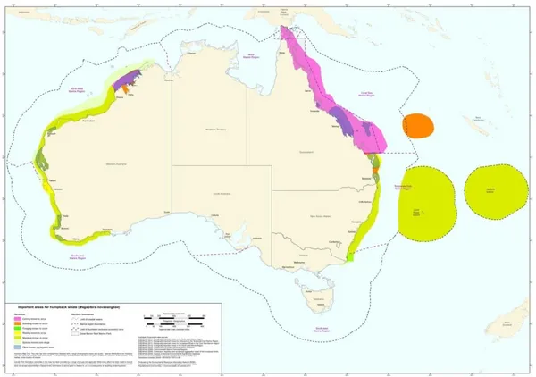
species. Humpback whales are known to undertake predictable migrations from high latitude where they forage in summer, to tropical grounds where they calve and breed (Clapham et al. 1993).They seem to exhibit high fidelity to these areas (Stevick et al. 2004) and to follow the same near shore migration corridors each year (Bryden 1985). For these reasons two different populations occur along Australia (Figure 2). The first population migrates on the eastern seaboard and mates and calves in the Great Barrier Reef (Smith et al. 2012) and the second population migrates along the western coast with calving and mating occurring off the Kimberley coast (Jenner et al. 2001). Recent genetic studies by Schmitt et al. (2014) show a lower differentiation between the two populations than the one expected due to the great spatial separation, suggesting that some individuals move between the two breeding grounds.
Figure 1: map showing humpback whales distribution around Australia: calving areas (pink), breeding areas (orange), foraging during migration (green), resting areas (yellow) source:
http://cutlass.deh.gov.au/coasts/species/cetaceans/australia/index.html
Feeding has long been considered to occur only in the highly productive polar regions where the two populations’ distribution is overlapped, but there is increasing evidence that this
13
behaviour occurs also during transit. Dawbin (1956) reported humpback whales feeding on euphausiids Nichtiphanes australis close to New Zealand in their northward migration, as well as feeding in surface plankton patches in their southward one. Gill et al. (1998) described the first confirmed humpback whales’ feeding behaviour in Tasmanian waters during their southward migration. Through the use of net tows samplings, it was also hypothesized that the whales were feeding on a mixed assemblage of zooplankton, which included aggregations of N. australis. Humpbacks were observed feeding on bait fish in low latitude waters around Moreton Island, Queensland (Stockin & Burgess 2005). More recently, Stamation et al. (2007) described observations of M. novaeangliae feeding along the south-eastern coast of New South Wales as reported by commercial whale watching boats. They found greater quantities of feeding events were recorded in years of higher productivity in the area, which was related to changes in the current systems. Gill et al. (1998) underlined that, as the energetic demand is quite high for migrating individuals, it is unsurprising that animals forage during their migration, especially as it may have been several months since they last fed.
Australia is also very important for these populations as it provides shallow-water, protected bays to mother and calf aggregations in the early stages of their southern migration. These areas are defined as resting grounds. On the east coast, Hervey Bay, Queensland (Franklin et al. 2011) and Jervis Bay, New South Wales (Bruce et al. 2014) are very important stopovers for females travelling with their calves before beginning their first long journey to Antarctica. The equivalent stopover sites on the west coast have being identified as Exmouth Gulf and Shark Bay (Jenner et al. 2001).
Pigmy blue whale
Balaenoptera musculus (Linnaeus, 1758) which can exceed 33 m in length and 180 t in
weight, is the biggest animal on earth (Yochem & Leatherwood 1985). Blue whales occur worldwide with 3 different subspecies . The Southern Hemisphere is known to host two of these subspecies: the Antarctic blue whale, Balaenoptera musculus intermedia and the pigmy blue whale, Balaenoptera musculus brevicauda.
The Antarctic blue whale is predominantly found in waters south of 60°S, while pigmy blue whales are mostly sighted north of 55°S (DEWHA 2008). For this reason, blue whales seen in waters around Australia are regarded as pigmy blue whales.
14
Information on seasonal distribution and movements of pigmy blue whales remains largely undocumented. It has been hypothesised that the animals occurring in Australia during summer months migrate to Indonesia following the western coast of Australia (Branch et al. 2007). Using satellite telemetry, Double et al. (2014) were able to describe the movements of some whales which indicated a migration following the western Australian coastline, leading to a possible breeding ground in Indonesia, reached by June.
Australia has been recognised as an important summer feeding ground (Figure 3) for the subspecies (Double et al. 2014). Many individuals aggregate each year to forage in two distinct feeding areas characterised by seasonal upwelling systems which support high prey densities (Gill 2002, Rennie et al. 2009). Pigmy blue whales are found off southern Australia between November-May, where they prey on the neritic euphausiid N. australis which concentrate in dense but patchy spots thanks to the nutrients brought to the surface by the Bonney Upwelling (Lewis 1981).
Figure 2: map showing pigmy blue whale use of Australian waters. Foraging areas (green), resting areas (yellow). Source:http://cutlass.deh.gov.au/coasts/species/cetaceans/australia/index.html
Through conducting aerial surveys, Gill et al. (2011) found that 23% of blue whales sighted in the region were feeding. Additionally, in 48% of these sightings, euphausiids surface swarms were identified in the surroundings (and the presence of submerged swarms cannot be excluded in the rest of them). The same study showed also a close association of whales
15
with upwelling surface plume visible fronts where they can probably find food more easily. It’s been estimated that the Bonney Upwelling feeding area (from Robe, South Australia, to Cape Otway, Victoria, and seawards to just beyond the shelf break) covers approximately 200000km² (Butler et al. 2002). Feeding blue whales have also been found in the eastern Great Australian Bight (GAB), indicating a significantly extended feeding ground in the southern Australia (Morrice et al. 2004). The second important feeding ground in Australian waters is found in the Perth Canyon, where pigmy blue whales aggregate between November and May (Rennie et al. 2009). This foraging area covers around 2300 km² (Department of the Department of the Environment 2015a).
Southern right whale
Eubalaena australis (Desmoulins, 1822) known as southern right whale, has several
populations with a circumpolar distribution in the southern hemisphere (Rice 1998). There is no spatial overlap between E. australis and the other two species of the genus Eubalaena, E.
glacialis and E. japonica. This could provide an explanation for the genetic differentiation
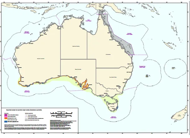
within the 3 different species of right whales, even if morphological and physiological characteristics have limited dissimilarities (Rosenbaum et al. 2000). This species was drastically exploited in the last two centuries and some populations might have been completely extirpated; while some populations seem to be recovering, others have not and there is ongoing concern for the preservation of their populations (Carroll et al. 2011). There remains a shortage of comprehensive knowledge on migratory routes, feeding and calving areas for the species (Department of the Environment 2015b). Australia is known to be an important breeding and calving area (Figure 4) for the species (Bannister 2001).
Dawbin (1986) hypothesised the existence of two different migration patterns from high latitude feeding grounds to Australia, where animals are seen from May to November. The study suggested that some whales migrate north along the east coast of Tasmania and then move up the coast of Victoria and New South Wales, while others migrate north along the west coast of Tasmania and then move westerly along the southern coast of South and Western Australia. Currently, only the second pattern is believed to occur (Carroll et al. 2011) with Warrnambool ( Victoria) considered to be the only calving area in the Southeast of the continent (Kemper et al. 1997).
16
Figure 3: map showing Southern right whale use of Australian waters. Calving areas (violet), breeding areas (orange). Source:http://cutlass.deh.gov.au/coasts/species/cetaceans/australia/index.html
Burnell and Bryden (1997) described the area at the Head of the Great Australian Bight, South Australia, as one of the largest, densest and most consistent aggregation areas in Australian waters for southern right whales. The same study investigated the difference in movements between calving and non-calving whales and found that unaccompanied whales spent significant less time in the area than females with calves, and that unaccompanied adults would leave and return to the area during a single season, probably for visiting other calving areas.
Bannister (1990) in an aerial counts study on southern right whales found a population increase in Southern-Western Australia and recorded both calving and mating, with reproduction occurring far from the coast.
17 2.4 Dwarf minke whale
Taxonomy
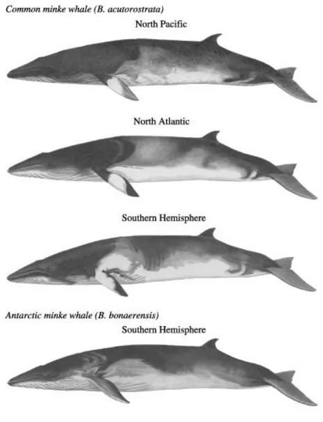
Minke whales are Mysticeti (baleen whales) of the genus Balaenoptera which includes blue, fin, sei, Bryde’s whales. Until recently, they were thought to be a single species with a cosmopolitan distribution (Murphy 1995). Rice (1998) reviewed morphological, genetic and osteological data for minke whales and suggested the separation into two species:
Balaenoptera acutorostrata (Lacépède,1804), the common minke whale occurring worldwide
and Balaenoptera bonaerensis (Burmeister, 1867), the Antarctic minke whale occurring only in the Southern Hemisphere. Furthermore, he recognised the North Atlantic B. acutorostrata
acutorostrata, North Pacific B. acutorostrata scammoni and Southern Hemisphere B. acutorostrata (unnamed) subspecies as three subspecies of the cosmopolitan minke whale
(Figure 5). B. acutorostrata (unnamed) subspecies is referred as dwarf minke whale and was first identify by Best ( 1985) as a diminutive form of southern minke whales, characterised by several diagnostic features such as coloration and dimensions. The International Whaling Commission recognised the two species in 2001 (IWC 2001), but has not yet listed the subspecies. Nevertheless, for management purposes it has been suggested that Antarctic and dwarf minke whale stocks should be regarded separately even if sympatric (Bannister et al. 1996, Acevedo et al. 2011).
Studying mitochondrial DNA, Pastene et al. (2010) found several populations of B.
acutorostrata subsp. in the Southern Hemisphere and suggested further examination of their
common sub-species status. The culmination of these factors and gaps in research has dictated the taxonomy of common minke whales to remain uncertain and yet to be determined (Reilly et al. 2008).
18
Figure 4: morphological differences between the three subspecies of common minke whale and the Antarctic minke whale.
Distribution
Dwarf minke whales have been recorded mostly in coastal habitat spanning the Southern Hemisphere in between 7° and 41°S, with sightings in South Africa (Best 1985), Australia (Arnold et al. 1987), New Zealand (Dawson & Slooten 1990) and South America (Zerbini et al. 1996). There have also been southern observations in the sub-Antarctic and Antarctic (Kasamatsu et al. 1993, Acevedo et al. 2011). Between April and October these animals are regularly seen in the Great Barrier Reef (Figure 6), where they are significantly relied upon for swim-with-whale programs (Birtles et al. 2002). Ninety per cent of the encounters in this area occurs in June and July (Birtles et al. 2014), while sightings in sub-Antarctic and Antarctic waters occur mainly between December and March (Kato et al. 1989, Kasamatsu et
19
al. 1993). The timing of these observations allow hypothesising a North/South migration from high latitude feeding grounds to mating and calving areas in the Tropics, but no large scale movement study has yet been conducted to test this theory (Pastene et al. 2010, Sobtzick 2010).
Figure 5: map of the Great Barrier Reef region where dwarf minke whales are encountered during Australian winter months (Sobtzick et al.,2010)
Abundance
Estimates of abundance and population size for dwarf minke whales do not exist. It has been reported that in the years from 1987/88 to 1998/99, 50 dwarf minke whales were sighted during the Japanese Research Whaling Program in the Antarctic (JARPA) surveys in the Indian/Pacific Ocean region and 16 of these were killed (Kato & Fujise 2000). Sobtzick (2010) indicated that the size of interacting individuals in the Great Barrier Reef consisted of several hundred animals each winter.
20 Biology
With a maximum recorded length of 7.8 m for females, 6.8 m for males and calves of around 2 m at birth (Best 1985, Birtles & Arnold 2008), dwarf minke whales are the smallest of the genus Balaenoptera.
The life span of these animals is unknown. Counting growth laminae on earplug core, Kato
and Fujise (2000) found an animal of aged 26 years and estimated a maximum value of roughly 46 years for the subspecies. However, the northern Hemisphere minke whales, which are currently considered the closest relative of the dwarf minke whale, live up to 60 years (Hoelzel & Stern 2000).
Dwarf minke whales present the most complex colouration of all mysticete (Arnold et al. 2005) and this can be used to distinguish single individuals with photo-identification as well as to discriminate within the two sympatric forms of minke whales in the Southern Hemisphere.
Studies on stomach contents revealed that the main prey found in animals around or north of 60°S were mychtophiids (Kato & Fujise 2000), but they are known to feed also on euphausiids (Zerbini et al. 1996, Secchi et al. 2003, Birtles & Arnold 2008), which suggests that the whales might be opportunistic feeders depending on the most abundant species they find (Kato & Fujise 2000).
2.5 Current study
While many baleen whale populations around Australia have been extensively studied and their migration routes are at least partially understood, there is a very limited knowledge base on the dwarf minke whale population wintering in the Great Barrier Reef (GBR). Migration towards Antarctic waters has been hypothesized, but not yet tested and no information exists about the presence of other significant areas in Australian waters for this population.
Chosen methods
To gain a deeper understanding of dwarf minke whale movements after their permanence in the GBR, some animals were equipped with satellite tags using Argos System to collect the data, before they started their displacement. This technology has been used in a variety of other studies on toothed and baleen whales (Andrews et al. 2008, Gales et al. 2012, Double et al. 2014, Vikingsson & Heide-Jorgensen 2015) as it provides reliable data for understanding large-scale movements and transmits locations directly to satellites without requiring devices
21
recovery. Using these locations, my project aims to understand dwarf minke whales use of Tasmanian waters during their southward migration. In order to answer this question, I will undertake 3 main steps: 1)along animals tracks, discriminate between areas of transit and longer residency, 2)characterise these areas’ environmental and oceanographic features, 3)create a model that correlates the time spent to the habitat characteristics.
The first step will require dividing the entire study area in 10km² cells and calculating the time spent by each individual in each cell, and then averaging it on the number of whales using the cell. The methodology of creating a grid to estimate the time spent by animals in different areas, has been used in several studies on cetacean distribution using satellite telemetry (Panigada et al. 2008, Gales et al. 2012, Double et al. 2014) as it is not affected by missing locations due to devices duty cycle or bad functioning.
Once areas of higher and lower residency are detected, importance will be given to understanding the environmental characteristics. As the tags did not collect any habitat information, I will use satellite derived and bathymetric data. Numerous variables have been used in cetacean studies to correlate their presence to particular habitat characteristics, but as highlighted by Hastie et al. (2005) the significance of these features varies between region and species, resulting in the importance of selecting environmental characteristics on a regional basis. For this reason, it will be important to assess which variable to include in the analysis, taking into account the particularities of the study area.
For the last step, I will model the relationships within the time spent by whales in each cell and each one of the variables extracted, using generalised additive models (GAMs). I will assume that the ex situ environmental data explanatory power does not differ significantly from in situ ones, as shown in Becker et al. (2010). Interpreting the model, it will be possible to determine the importance of particular environmental parameters in whales’ habitat use and speculate on what is the biological reason of this different use, either for foraging or resting reasons.
22 3. Scientific paper
Abstract
The Great Barrier Reef hosts the only known reliable aggregation of dwarf minke whale (Balaenoptera acutorostrata subspecies) in Australian waters. While this short seasonal aggregation is quite predictable, the distribution and movements of the whales during the rest of their annual cycle are poorly understood. In particular, feeding and resting areas on their southward migration which are likely to be important have not been described. Using satellite telemetry data, I modelled the habitat use of seven whales during their southward migration through waters surrounding Tasmania. The whales were tagged with LIMPET satellite tags in the GBR in July 2013 (2 individuals) and 2014 (5 individuals). The study area around Tasmania was divided into 10km² cells and the time spent by each individual in each cell was calculated and averaged based on the number of animals using the cell. Two areas of high residency time were highlighted: south-western Bass Strait and Storm Bay (SE Tasmania). Remotely sensed ocean data were extracted for each cell and averaged temporally during the entire period of residency. Using Generalised Additive Models I explored the influence of key environmental characteristics. Nine predictors (bathymetry, distance from coast, distance from shore, gradient of sea surface temperature, sea surface height (absolute and variance), gradient of current speed, wind speed and chlorophyll-a concentration) were retained in the final model which explained 68% of the total variance. Regions of higher time-spent values were characterised by shallow waters, proximity to the coast (but not to the shelf break), high winds and sea surface height but low gradient of sea surface temperature. Given that the two high residency areas corresponded with regions where other marine predators also forage in Bass Strait and Storm Bay, I suggest the whales were probably feeding, rather than resting in these areas.
23 3.1 Introduction
Many species of baleen whales migrate annually from high latitude summer foraging grounds to tropical mating and breeding grounds during winter (De Sá Alves et al. 2009). Migration routes were once regarded as simple corridors crossed by animals to reach the two most important areas, but the importance of these routes is being re-evaluated with increased appreciation of the degree of opportunistic feeding (Stamation et al. 2007) and resting behaviours (Bruce et al. 2014).
The conservation and management of highly migratory species whose migration routes are poorly understood, as is the case for many cetaceans, is a significant challenge (Hyrenbach et al. 2000). Consequently, studies that explore whale movements during migration and their habitat use are of particular relevance as they can enrich knowledge on species’ ecology as well as distinguish critical habitats, defined as the habitats necessary for the persistence of a population, thus feeding, breeding grounds and common migratory routes (Gregr & Trites 2001). Moreover, they can reveal potential direct and indirect negative human impacts on animals or their environment and resources, and thus guide appropriate management and conservation efforts (Redfern et al. 2006).
Habitat modelling techniques have proven to be effective tools to understand how species distributions are related to environmental characteristics (Hastie et al. 2005, Panigada et al. 2008, Pirotta et al. 2011) and have therefore been used to gain a deeper knowledge on species ecology, habitat use and to predict distribution patterns (Redfern et al. 2006). Bathymetric and oceanographic features are often used as proxies of other factors which are likely to have a significant and direct influence on animal movements and distribution but are not easily quantifiable, such as prey availability, interspecific relationships, competition, predation risk and behavioural needs (Pirotta et al. 2011).
The development of habitat models requires data on animal distribution, which can be difficult to obtain for cetaceans due to the environment where they live and the elusive nature of their behaviour (Redfern et al. 2006). Traditional techniques including land-based, ship and aerial visual surveys can provide data on cetacean presence and distribution on very small portions of their total habitat range (e.g. Barlow & Taylor 2005, Tynan et al. 2005, Bruce et al. 2014). The more recent satellite telemetry is considered the most efficient option
24
whenever fine-scale and long-term movement data are necessary (Gillespie 2001). Relying on devices temporarily deployed on animals, it is often utilised to understand cetacean migratory patterns (e.g. Double et al. 2014, Vikingsson & Heide-Jorgensen 2015) and habitat use (e.g. Andrews et al. 2008, Gales et al. 2012).
Tagging, distribution studies and whaling records from the past have demonstrated the importance of south-eastern Australian waters for several species of baleen whales. Humpback whales, Megaptera novaeangliae, migrate along the east coast of Australia to reach high latitude foraging grounds (Chittleborough 1965, Stevick et al. 2004, Stamation et al. 2007). In particular, their migration routes encompass Tasmanian waters both on the east and west coasts and there are regions around the island where they pause their migration and spend days to weeks (Gales et al. 2009). Catch reports of southern right whales, Eubalaena
australis suggested the existence of two different migration patterns from high latitude
feeding grounds to Australia with some animals migrating north along the east coast of Tasmania and then moving up the coast of Victoria and New South Wales, and others migrating north along the west coast of Tasmania and then moving westerly along the southern coast of South and Western Australia (Dawbin 1986). Currently, only the second pattern seems to occur (Carroll et al. 2011) with Warrnambool (Victoria) considered to be the only calving area in the Southeast of Australia(Kemper et al. 1997). In contrast, pigmy blue whales Balaenoptera musculus brevicauda use south-east Australia for feeding purposes, aggregating in the surrounding of the Bonney Upwelling to prey on dense but patchy krill aggregations (Gill 2002).
The use of south-eastern Australian waters by dwarf minke whales Balaenoptera
acutorostrata undescribed subspecies wintering in the Great Barrier Reef is poorly
understood. A north-south movement from high latitude feeding grounds to mating and calving areas in the tropics has been hypothesized because of the timing of sightings in sub -Antarctic and -Antarctic waters, which occur mainly between December and March (Kato et al. 1989, Kasamatsu et al. 1993) and in warmer waters, which occur mainly between April and October (Arnold et al. 1987, Birtles & Arnold 2008). Ninety percent of dwarf minke whales in the Great Barrier Reef, the world’s only predictable aggregation of this subspecies, occur between June and July (Birtles et al. 2014). No large scale movement study has been done to prove this migration pattern (Pastene et al. 2010, Sobtzick 2010) and considering the deficiency of knowledge on global population size and conservation status for this
25
undescribed subspecies, addressing questions on biology and spatial ecology of dwarf minke whales it’s of primary importance to protect the subspecies and identify where critical areas are and whether any overlap with anthropogenic threats occur or is likely to occur.
In order to provide insights into dwarf minke whale migration routes and their use of south-eastern Australian waters, this study combined satellite telemetry data with habitat modelling techniques. The objective of this study was therefore to understand how individuals from the dwarf minke whale population wintering in the Great Barrier Reef, used waters surrounding Tasmania, assessing the presence of areas of particular importance during their southward migration. Specifically, I aimed to: i) quantify the dissimilarities in time-spent in different regions of the study area; ii) determine what environmental features characterised these regions; and iii) find regional differences between the environmental characteristics in the higher time-spent areas. The results of this study will provide the first baseline information on dwarf minke whales habitat use in Tasmanian waters.
3.2 Materials and methods Tag deployment
An estimated population of several hundreds of dwarf minke whales seasonally occur in the Great Barrier Reef Marine Park, Queensland. Whales visiting the waters surrounding Lizard Island in the northern region of the Great Barrier Reef Marine Park (Figure 6) in July 2013 (n=4) and 2014 (n=10) were tagged by in-water researchers using modified spear guns using tags in the Low-Impact Minimally Percutaneous External Transmitter (LIMPET) configuration (Andrews et al. 2008) . The tags were SPOT (location-only, 55x35x22 mm) and SPLASH (location/dive tags, 57x45x26 mm) tags (Wildlife Computers, Redmond, WA, USA). The satellite tags had two sub-dermal attachments and a 17cm long antenna and maximum mass of 69 grams.
26
Figure 6: map showing the study area. The inserted map of Australia shows the tagging area in the circle.
Tracking data processing
Satellite position estimates received from the Service Argos have an estimated error associated with them ranging from 250 m to >1.5 km (location class 3, 2, 1, 0, A, B) (Argos user's manual, 2011). To remove unlikely locations, the plausibility of each position estimate was assessed using the Douglas Argos Filter v.8.05 (Douglas et al. 2012), which is a systematic algorithm that considers different user-defined thresholds for location class, swimming speeds, distances between successive locations and turning angles to filter the locations. The filter was set to retain all locations with location classes of 3 or 2 or within a distance <3 km from the immediately previous or subsequent location, all other locations were subject to filtering. These locations were removed if the rate of movement between consecutive locations was higher than 25 km/h or if the angle between 3 subsequent locations was unrealistic (Andrews et al. 2008).
Data analysis
The data analysis was performed using R (R Development Core Team, 2015) version 3.1.3. The entire tracking dataset was subset to include only locations around Tasmania within longitude 140°E to 150°Eand latitude 34°S to45°S (Figure1). I first analysed the animal movements by plotting the tracks and producing heatmaps showing the latitudinal and longitudinal positions along time. Using the package ‘sp’ version 1.1-0 (developed by
27
Pebesma et al., 2015) the distance between animals occurring in the study area in similar days was calculated as the distance between an average position for each animal each day.
Time-spent analysis
The entire study area was divided in 10x10km grids by using the package ‘trip’ (developed by Sumner, 2011) to enumerate how the whales spent their time in the area. The 10-km spatial scale was chosen after trying different grid dimensions, and was found to be the best for identifying whales residency in an area (Dalla Rosa et al. 2012, Double et al. 2014). The total time spent by each individual whale in each cell was calculated. Then, this was averaged amongst whales within each cell. A spatial smoother was applied to reduce the noise component due to possible different spatial resolutions between the whales’ tracks and the environmental covariates extracted in the subsequent steps. The smoothing process involved initially aggregating 3 cells by 3 cells by their time-spent mean value, and then resampling them with again 10km2 cells.
Environmental data
Environmental covariates were extracted for the entire study domain using the Rpackage ‘Raadtools’ version 0.2-5 (developed by Sumner, 2015) (Table 2). Remotely
sensed data for each variable that I planned to consider for the entire study period were derived at the finest temporal and spatial resolution available and then averaged to create a single raster for each covariate that showed the mean values of the variable over the total time of the study. Finally, a single value for each of the environmental covariates was attributed to each of the cells used by the whales producing the dataset utilised in the statistical modelling. The variables extracted have proven valuable in other studies on marine mammal distribution and habitat use, showing specific correlations with the presence of animals varying with the species, the ocean basin and the natural history of the organism. Bottom depth (bathy) and topographic characteristics, which include distance to the coast (dscst) and to the shelf break (dsshb), have proven to be important proxies for general habitat suitability (Kaschner et al. 2006) as related to prey bathymetric zonation (Pirotta et al. 2011) or social behaviour needs (Franklin et al. 2011). Sea surface temperature (SST), gradient of sea surface temperature (gSST), sea surface height (SSH), sea surface height variance (vSSH) can provide information on upwelling and other oceanographic processes that enhance primary productivity and thus sustain rich trophic webs (Tynan et al. 2005) which are likely to attract foraging animals. Similarily, chlorophyll-a concentration (chl-a) is an indicator of primary productivity (Dalla
28
Rosa, 2012). Winds (wind) and currents (gcurr) can influence water vertical stratification affecting vertical migration and surface patchiness of prey species (Littaye et al. 2004) targeted by whales.
Covariate Unit Source Spatial scale Temporal
scale
Chlorophyll-a mg/m3 Calculated with Johnson et al. (2013) algorithm from MODIS/Aqua Level-3-binned data
http://oceancolor.gsfc.nasa.gov/
4.63x4.63km Daily
Sea surface temperature
°C NOAA Optimum Interpolation ¼ Degree Daily Sea Surface Temperature Analysis
http://www.ncdc.noaa.gov/oa/climate/research/sst/oi-daily-information.php
0.25 × 0.25° Daily
Sea surface
temperature gradient
°C Calculated from extracted sea surface temperature values using the Rpackage ‘raster’ (Hijmans et
al.,2015)
/ /
Sea surface height m AVISO
http://www.aviso.oceanobs.com/en/data/products/sea -surface-height-products/global/index.html
0.25 × 0.25° Daily
Sea surface variance m Calculated from extracted sea surface height values using the Rpackage ‘raster’ (Hijmans et al.,2015)
/ /
Currents magnitude m/s SSALTO/DUACS - DT Geostrophic Velocities - Up-to-date Global Processing
http://www.aviso.oceanobs.com/en/data/products/sea -surface-height-products/global/index.html
0.25 × 0.25° Daily
Currents gradient m/s Calculated from extracted currents magnitude values using the Rpackage ‘raster’ (Hijmans et al.,2015)
/ /
Wind speed m/s NCEP 2
http://www.esrl.noaa.gov/psd/data/gridded/data.ncep .reanalysis.derived.surface.html
2.5x2.5° Daily
Bathymetry m GEBCO_2008 Grid
http://www.gebco.net/data_and_products/gridded_ba thymetry_data/gebco_update_history/version_20100 927/ 30x30arc-second /
Distance from shelf break
km Calculated from extracted bathymetric values / /
Distance from coast km Calculated from extracted bathymetric values / /
Table 2: environmental covariates derived or calculated from satellite repository dataset with their unit, source and spatial and temporal resolution.
29 Statistical modelling
A generalized additive modelling framework was used to assess the relationships between the mean time-spent in each cell and its environmental variables. Such models are commonly applied in ecological studies (Hastie et al. 2005, Friedlaender et al. 2006, Pirotta et al. 2011) because they don’t impose limitations on the form of the relationships within a response variable (in this case the time-spent) and a series of predictors (the environmental characteristics) (Hastie & Tibshirani 1990). For the purpose of this thesis, to avoid the use of unnecessary overcomplicated modelling techniques, it was decided not to include any term to deal with spatial auto-correlation issues, intrinsic to the dataset. Further data analysis will be undertaken with the collaboration of statisticians to implement the data frame here utilised. The variables were first centred around their mean. Their distribution was checked plotting histograms for each one. Only the response variable (mean time-spent) required log transformation to gain distribution normality. Outlying values of chl-a greater than 4 mg/cm³ were removed to avoid undue leverage (Zuur et al. 2007). I also tested Pearson’s correlation among variables to avoid collinearity which might have affected the model performances resulting in overfitting the data without detecting the effective relationships among response variable and predictors (Zuur et al. 2007). When two variables were highly correlated (|r|>0.8) the variable with lower temporal or spatial resolution was not included in the modelling.
The mgcv package version 1.8-6 (developed by Simon Wood, 2015) of the R program was
used in the modelling. First, a single generalised additive model (family: Gaussian, link function: identity) for each possible predictor was built to assess the importance of each factor in determining the mean time-spent. More complex GAMs were produced including all the variables and removing one variable per time in a backward stepwise selection (Zuur et al. 2007) and assessing which variables had to be retained in the final model by comparing the AICs (Akaike 1987).
Finally, smoothed GAM plots were used to visualize the relationship between each predictor and the response variable. The flexibility of GAMs can lead to an overfit of the data (Hastie et al. 2005), making it essential to approach the interpretation of distribution-environment relationships with caution. When interpreting the plots, I focused on the portion of the curve
30
where the majority of the sample points were, that is where I have a higher confidence due to the narrower confidence intervals.
Regional comparisons
Once the most informative environmental covariates were selected using the GAM, I assessed the importance of each of them in the different high residency areas, in particular Bass Strait and southern Tasmania. Cells were divided into ‘high use’ and ‘low use’ bins based on the 75% quantiles mean time-spent, where 0-75% quantiles corresponded to low use and 75-100% quantiles to high use. For each variable, boxplots were produced to compare values between ‘high use’ and ‘low use’ cells in the north and south regions.
31 3.3 Results
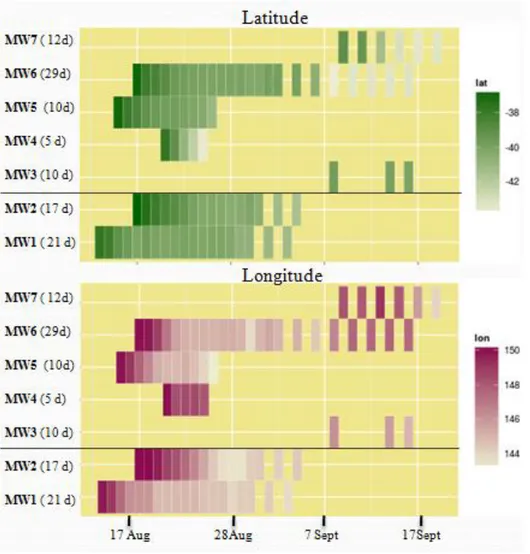
Some tags stopped transmitting after less than 50 days, when the whales were still following the eastern coast of mainland Australia. Seven whales transmitted for long enough to reach south-eastern Australia,(n=2 in 2013, n=5 in 2014) and were included in the analysis as they spent considerable time in waters surrounding Tasmania. All of them carried SPOT location-only tags. The seven whales spent from 5 to 29 days in the area, While in the study area, five of the tags switched from a schedule in which they transmitted every day to a duty cycle in which they did not transmit every day in order to conserve battery power for attachments that exceeded the number of consecutive transmission days that the battery could provide power for. Four tags stopped transmitting while the whale was still in the study area (Figure 7).
Figure 7: heatmaps showing whales movement in latitude (decreasing green intensity= decreasing in latitude) and longitude (decreasing purple intensity= decreasing in longitude). On the left the name of the animal and number of days spent in the study area, the black line separates animals from 2013 and 2014. On the y-axis the day, each rectangle represents a day spent in the study area. Clear is the start of duty cycle for some tags.
32 Dwarf minke whales movements
Once the whales arrived at the northern end of Bass Strait, different routes were chosen: (i) the majority of them (2 whales in 2013 and 3 whales in 2014) crossed Bass Strait in a westward direction, spent some time in between King Island and north-west Tasmania where they moved in a less clear and straight way, or moved out of the study area heading south or followed the Tasmania western coast reaching Storm Bay (1 animal),(ii) two whales moved south following the Tasmania eastern coast (Figure 8).
Figure 8 : whales tracks, in red animals tagged in 2013, in blue animals tagged in 2014.
The mean distance on a given day between the two whales in 2013 was 223.7 km (s.e. 51.5 km), with a minimum recorded distance of 21.7 km. The mean distance between animals in 2014, not including the distances between animals on the opposite sites of the island, was 309.1 km (s.e. 33.7 km), with a minimum recorded distances of 16.8 km, 305.7 km, 239.8 km between pairs of animals.
33 Time-spent analysis
A total of 785 10 km² cells were used by at least one whale, with 2 cells being used by 5 whales and 16 used by 4 whales (Figure 9). Approximately 68 hours was the maximum time spent in a single cell by a single whale. The time-spent analysis averaged on all the individuals clearly highlighted the presence of areas with higher residency time compared with the surrounding areas: the maximum value was 22 hours spent by whales in a cell. The higher values of time-spent were recorded in central-western Bass Strait and Storm Bay. In contrast, the time-spent in cells along the east and west coast of Tasmania was considerably lower, with values varying from 3 to 10 hours.
Figure9: a) map showing the hours spent per cell of 10x10km, red cells indicate higher time spent. b) map showing the number of animals that used each cell during the two years combined.
34 Statistical modelling
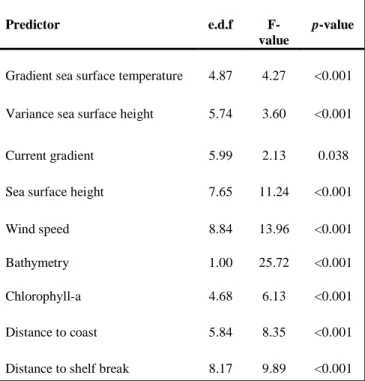
The use of GAMs suggested that several environmental variables influenced the amount of time spent by whales in an area: gSST, SSH, vSSH, chl-a, gcurr, wind, bathy, dscst and dsshb were all found in the final model. Only bathy showed a linear relationship with the time-spent, while all the other values were clearly non-linear. The final model explained 67.9% of variance. The majority of smoothed variables were highly significant with p-values <0.001 (Table 3).
Predictor e.d.f
F-value
p-value
Gradient sea surface temperature 4.87 4.27 <0.001 Variance sea surface height 5.74 3.60 <0.001
Current gradient 5.99 2.13 0.038
Sea surface height 7.65 11.24 <0.001
Wind speed 8.84 13.96 <0.001
Bathymetry 1.00 25.72 <0.001
Chlorophyll-a 4.68 6.13 <0.001
Distance to coast 5.84 8.35 <0.001 Distance to shelf break 8.17 9.89 <0.001
Table 3: estimated degrees of freedom (e.d.f), F-values and p-values for each smoothed predictor as evaluated during the modelling.
There was a generally negative relationship between gSST, dscst and mean time-spent in a cell (Figure 10). Bathy had a linear positive effect, with whales spending more time in shallow waters. SSH and wind displayed bimodal relationship with mean time-spent, which increased with mid and high values of the two predictors. Dsshb and chla-a were generally positively related to mean time-spent. While contributing to the final model, there was no obvious relationship between SSH and gCurr and mean time-spent.
35
Figure 10: Generalized additive model functions of dwarf minke whales time spent in relation to environmental variables. Continuous lines: smoothing curve; grey shading: 95% confidence limits. x-axis = centred variable, y-axis fitted smooth function; along x-axis indicate individual sample points.
36 Regional comparisons
The regional comparisons highlighted important differences between the northern and southern regions. gSST and bathy had similar relationships to mean time-spent in the two regions, with high time-spent cells characterised by lower values of the two variables (Table 4). In contrast, chl-a and dsshb had opposite relationships with mean time-spent in the north and south, with high time-spent cells in the south characterised by high values of chl-a and low dsshb, and high time-spent cells in the north showing low values of chl-a and high dsshb.
SSH, vSSH, gcurr and dscst values did not show significant differences in high and low
time-spent in the north, but were important in discriminating the use of cells in the south. Oppositely, wind values differed between high and low time-spent cells in the north but not in the south.
Table 4: differences between the correlation of each variable with low time spent (cold) and high time spent (hot) cells in the north and south regions, where the separation was determined by using lat=42°S as threshold
NORTH SOUTH
Variables COLD HOT COLD HOT
Gradient SST + - + -
Sea surface height = = + -
Variance sea surface height = = - +
Bathymetry + - + -
Wind speed - + = =
Current gradient = = + -
Chlorophyll-a + - - +
Distance coast = = + -