Scuola di Scienze
Corso di Laurea Magistrale in Fisica
Multicentre study for a robust protocol in
single-voxel spectroscopy: quantification of
MRS signals by time-domain fitting
algorithms
Relatore:
Prof.ssa Paola Fantazzini
Correlatori:
Dott.ssa Paola Berardi Dott.ssa Emma Fabbri
Presentata da: Nicola Mordini
Sessione II
La Spettroscopia di Risonanza Magnetica (MRS) `e un’applicazione avanzata cli-nica e di ricerca che consente una specifica caratterizzazione biochimica e meta-bolica dei tessuti tramite l’identificazione e la quantificazione di metaboliti chiave per la diagnosi e la stadiazione della malattia.
L’ ”Associazione Italiana di Fisica Medica (AIFM)” ha promosso l’attivit´a del gruppo di lavoro ”Interconfronto di spettroscopia in RM”. Lo scopo dello studio `e il confronto e l’analisi dei risultati ottenuti dall’esecuzione di MRS su scanner di diversi ospedali per redigere un protocollo robusto per esami spettroscopici per la pratica clinica. Questa tesi s’inserisce nel progetto tramite l’utilizzo dello scanner GE Signa HDxt 1.5 T presso il Padiglione 11 dell’Ospedale S.Orsola-Malpighi di Bologna.
Le analisi degli spettri, acquisiti su due distinti fantocci, sono state eseguite con il pacchetto jMRUI, che offre una vasta gamma di algoritmi di preprocessing e quantificazione per l’analisi di segnali nel dominio del tempo. Dopo il controllo di qualit´a con metodi standard e innovativi, sono stati acquisiti spettri con e senza soppressione dell’acqua sul fantoccio di prova GE. Il confronto fra i rapporti delle ampiezze dei metaboliti rispetto alla Creatina calcolati dal software della workstation, che opera sulle frequenze, e da jMRUI mostrano un buon accordo, suggerendo che le quantificazioni in entrambi i domini possano condurre a risultati consistenti.
La caratterizzazione di un secondo fantoccio, fornito dal gruppo di lavoro, ha raggiunto il proprio obiettivo, cio´e la valutazione del contenuto della soluzione e delle concentrazioni dei metaboliti con buona accuratezza. La bont´a della proce-dura sperimentale e dell’analisi dati `e stata dimostrata dalla corretta stima del T2 dell’acqua, dall’osservazione della curva di rilassamento biesponenziale della
Creatina e dal corretto valore del TE in corrispondenza del quale la modulazione del J coupling causa l’inversione del doppietto del Lattato nello spettro.
Il lavoro di questa tesi ha dimostrato che `e possibile eseguire misure e pianificare protocolli per l’analisi dati, basati sui principi NMR, che possano fornire valori robusti per i parametri dello spettro di uso clinico.
Magnetic Resonance Spectroscopy (MRS) is an advanced clinical and research application which guarantees a specific biochemical and metabolic characterization of tissues by the detection and quantification of key metabolites for diagnosis and disease staging.
The ”Associazione Italiana di Fisica Medica (AIFM)” has promoted the activ-ity of the ”Interconfronto di spettroscopia in RM” working group. The purpose of the study is to compare and analyze results obtained by perfoming MRS on scanners of different manufacturing in order to compile a robust protocol for spec-troscopic examinations in clinical routines. This thesis takes part into this project by using the GE Signa HDxt 1.5 T at the Pavillion no. 11 of the S.Orsola-Malpighi hospital in Bologna.
The spectral analyses have been performed with the jMRUI package, which includes a wide range of preprocessing and quantification algorithms for signal analysis in the time domain. After the quality assurance on the scanner with standard and innovative methods, both spectra with and without suppression of the water peak have been acquired on the GE test phantom. The comparison of the ratios of the metabolite amplitudes over Creatine computed by the worksta-tion software, which works on the frequencies, and jMRUI shows good agreement, suggesting that quantifications in both domains may lead to consistent results.
The characterization of an in-house phantom provided by the working group has achieved its goal of assessing the solution content and the metabolite concen-trations with good accuracy. The goodness of the experimental procedure and data analysis has been demonstrated by the correct estimation of the T2 of water,
the observed biexponential relaxation curve of Creatine and the correct TE value at which the modulation by J coupling causes the Lactate doublet to be inverted in the spectrum.
The work of this thesis has demonstrated that it is possible to perform measure-ments and establish protocols for data analysis, based on the physical principles of NMR, which are able to provide robust values for the spectral parameters of clinical use.
Introduzione 1
1 Magnetic Resonance Spectroscopy 5
1.1 The physical basis . . . 5
1.1.1 A brief history . . . 5
1.1.2 The Larmor resonance frequency . . . 6
1.1.3 Chemical shift . . . 8
1.1.4 J coupling . . . 10
1.1.5 Nuclear Overhauser effect . . . 15
1.1.6 Spectrum formation . . . 17
1.2 Magnetic field gradients in MRI and MRS . . . 25
1.2.1 Field gradients in MRI . . . 25
1.2.2 Field gradients in MRS . . . 27
1.3 Single-volume localization sequences . . . 31
1.3.1 Selective pulses and relaxation times . . . 31
1.3.2 ISIS . . . 32
1.3.3 STEAM . . . 34
1.3.4 PRESS . . . 36
1.3.5 Imperfect RF pulses . . . 38
1.3.6 Signal suppression methods . . . 39
1.3.7 Non-water-suppressed MRS . . . 43
1.4 Chemical shift imaging . . . 44
1.4.1 Multi-voxel techniques . . . 44 i
1.4.2 Comparison of single-voxel and CSI techniques . . . 45
2 MRS applications in diagnostic medicine 47 2.1 MRS clinical studies . . . 47
2.1.1 Diagnostic utility of MRS . . . 47
2.1.2 Clinical relevance of 1H MRS studies . . . . 48
2.1.3 Principal metabolites in 1H MRS . . . . 51
2.1.4 Temperature dependence of the water peak position . . 58
2.1.5 31P MRS studies . . . . 60
2.1.6 13C MRS studies . . . . 63
2.2 Biological effects related to magnetic field exposure . . . 63
2.2.1 Interactions of magnetic fields with human tissues and safety . . . 63
2.2.2 Tissue heating . . . 65
3 Data acquisition system and instrumentation 67 3.1 The MR scanner . . . 67
3.1.1 Characteristics of GE Signa HDxt 1.5 T scanner . . . . 67
3.1.2 GE Signa HDxt 1.5 T workstation . . . 69
3.2 Additional instrumentation . . . 72
3.2.1 Head coil . . . 72
3.2.2 GE spherical test phantom . . . 74
3.2.3 In-house phantom . . . 76
4 Spectroscopic quality assurance 77 4.1 Concerns in MRS quality control . . . 77
4.1.1 The compiling of the acceptance report . . . 77
4.1.2 Image quality . . . 78
4.1.3 Spectral quality . . . 79
4.2 Quality assurance on GE spherical phantom . . . 81
4.2.1 Signal localization . . . 81
4.2.3 Estimation of image uniformity . . . 86
4.2.4 Dependence of the signal intensity on the excited volume 87 4.2.5 Evaluation of the homogeneity of the static and the RF magnetic fields . . . 89
4.2.6 SNR and concentration measurements in the spectra . 93 5 Time-domain preprocessing and fitting algorithms 97 5.1 Time-domain quantification . . . 97
5.1.1 Comparison of spectral analysis in the time domain and in the frequency domain . . . 97
5.1.2 Quantification in the time domain . . . 98
5.1.3 Introduction to the jMRUI software . . . 99
5.2 A noniterative algorithm: HLSVD . . . 102
5.2.1 Singular value decomposition of a Hankel matrix . . . . 102
5.2.2 Application of the Lanczos algorithm to the Hankel matrix . . . 104
5.3 An iterative algorithm: AMARES . . . 105
5.3.1 Fitting of the nonlinear model function by least-mean-square method . . . 105
5.3.2 Maximum likelihood estimates . . . 106
5.3.3 Prior knowledge in AMARES . . . 108
6 Analyses of the water peak 109 6.1 Quantification of the water peak and experimental settings . . 109
6.1.1 The usefulness of non-water-suppressed spectra . . . . 109
6.1.2 Experimental settings and parameters . . . 110
6.1.3 Quantification operations and error estimation . . . 111
6.2 Results of quantification of spectra without water suppression 114 6.2.1 Signal response for VOIs at different positions . . . 114
6.2.2 Quantification of the water peak at increasing VOI di-mensions . . . 117
6.2.3 Quantification of the water peak at varying TEs and
T2 relaxation time extrapolation . . . 120
7 Quantification of metabolite spectra 123 7.1 Residual water peak removal from the metabolite spectrum . . 123
7.1.1 HLSVD peak remover . . . 123
7.1.2 Effects of the removal of the water peak from the metabo-lite spectrum . . . 125
7.2 Quantification of metabolite amplitudes by AMARES . . . 127
7.2.1 Peak picking on the spectrum . . . 127
7.2.2 Metabolite amplitude quantification settings and oper-ations . . . 128
7.2.3 Results of the quantification of metabolite peaks . . . . 131
8 Characterization of the in-house phantom 137 8.1 Spectral analyses . . . 137
8.1.1 Identification of the phantom content by MRS . . . 137
8.1.2 Quantification of the solvent . . . 138
8.1.3 Quantification of the solutes . . . 142
8.2 Internal concentration reference method . . . 149
8.2.1 Water content estimation . . . 149
8.2.2 Determination of metabolite concentrations . . . 150
Conclusions 153
Bibliography 155
1.1 Electron shielding of the nucleus. . . 8
1.2 Different shielding in the acetaldehyde molecule. . . 10
1.3 Rearrangement of nuclear and electronic spins through J cou-pling. . . 12
1.4 Resonance peaks of two coupled spins. . . 14
1.5 Roof effect in strongly-coupled spins. . . 14
1.6 Energetic level and transition diagram for two uncoupled spins exhibiting nuclear Overhauser effect. . . 16
1.7 Precession of magnetization in the rotating frame when the RF pulse is off-resonant. . . 18
1.8 Free induction decay following an excitation pulse. . . 19
1.9 Lorentzian lineshape in the frequency domain. . . 20
1.10 Spectrum and covalent structure of Lactate. . . 22
1.11 Filtering of the FID through weighting function for noise re-duction. . . 23
1.12 Lorentzian and Gaussian resonance lines of equal FWHM and integrated amplitude. . . 24
1.13 Position and frequency ranges excited through slice-selective gradient. . . 26
1.14 Fat voxel offset location with respect to the water voxel. . . . 29
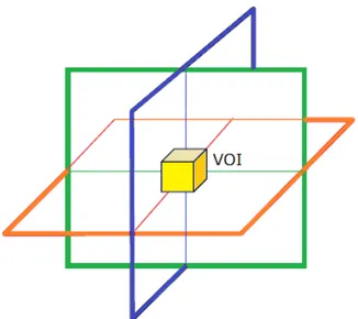
1.15 Defined VOI from intersection of the three slice-selective RF pulses applied in orthogonal directions. . . 31
1.16 Pulse sequence for ISIS. . . 33 v
1.17 Pulse sequence for STEAM. . . 35
1.18 Pulse sequence for PRESS. . . 37
1.19 Spatial localization by PRESS pulses. . . 38
1.20 CHESS water suppression sequence repeated three times. . . . 40
1.21 Pulse sequence for WEFT. . . 41
1.22 Null point for water magnetization after the application of a 180◦ pulse. . . 42
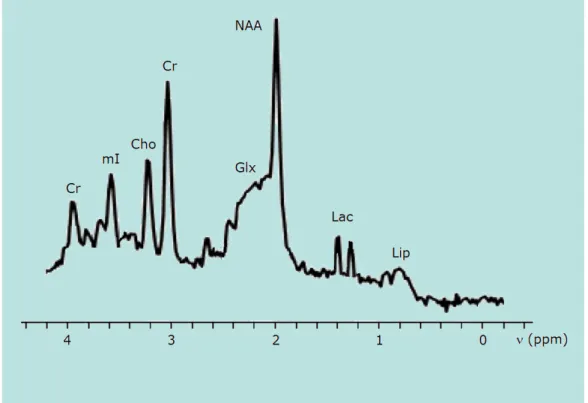
2.1 In vivo proton spectrum of the main metabolites with fre-quency range of 4 ppm. . . 49
2.2 Chemical structure of N-acetyl aspartate. . . 52
2.3 Chemical structure of Choline. . . 53
2.4 Creatine kinase reaction. . . 54
2.5 Chemical structure of Lactate. . . 54
2.6 Proton spectra acquired using PRESS at 30 ms and 150 ms displaying the inversion of Lac doublet. . . 56
2.7 Chemical structure of Myo-Inositol. . . 56
2.8 Chemical structures of Glutamate and Glutamine. . . 57
2.9 In vivo phosphorous spectrum of the main metabolites with frequency range of 30 ppm. . . 60
2.10 Chemical structure of ATP with its three phosphate groups. . 62
3.1 GE Signa HDxt 1.5 T. . . 68
3.2 Monitor screen for protocol downloading. . . 70
3.3 GE 1.5 T MRI classic quad head coil no. 2384268. . . 73
3.4 GE spherical test phantom with its base. . . 74
3.5 In-house phantom with its measuring cylinder for filling. . . . 76
4.1 Examples of axial, sagittal and coronal scout images. . . 81
4.2 Images of the whole phantom, the selected ROI and the local-ization of the ROI within the phantom. . . 82
4.4 Signal and noise ROIs in the spin-echo image and in the
sub-traction image. . . 84
4.5 Selection of concentric square ROIs at the centre of the phantom. 87 4.6 Proportionality of the total signal intensity at varying ROI areas. . . 89
4.7 Steps in mm in the displacement of the selected ROI along the A/P and R/L axes. . . 90
4.8 ROI signal intensity along the A/P axis. . . 91
4.9 ROI signal intensity along the R/L axis. . . 92
4.10 STEAM and PRESS spectra acquired during QA. . . 96
5.1 A water signal viewed in the time domain (top), in its absolute value (black) (middle )and in its real and imaginary compo-nents (red and green) (bottom) in the frequency domain on jMRUI-5.1 time-series screen. . . 101
6.1 From bottom to top: Original, estimated, individual compo-nents and residue spectra viewed on the HLSVD result window over a non-water-suppressed spectrum. . . 112
6.2 VOIs selected at different locations in the axial image. . . 114
6.3 Amplitude linear trend at increasing VOI dimensions. . . 118
6.4 Linear trend of the water peak linewidth at increasing VOI dimensions. . . 119
6.5 Amplitude exponential decay of the water peak in function of TE. . . 122
7.1 jMRUI screen views of the spectrum before the application of HLSVD peak remover (top), the zoomed selected frequency region for elimination (middle) and the spectrum after the pro-cessing and the shifting of the reference zero frequency (bottom).126 7.2 jMRUI screen views of a metabolite spectrum acquired by PRESS before (top) and after the Gaussian apodization (bot-tom). . . 130
7.3 jMRUI screen views of the peaks picked on a QA spectrum (top) and the graphical results by AMARES (bottom). . . 132 8.1 VOI positioning in the axial image of the in-house phantom. . 140 8.2 Water peak amplitude in function of TE values. . . 141 8.3 GE workstation (top) and jMRUI screen views (bottom) of
the metabolite spectrum acquired at TE = 35 ms. . . 144 8.4 Creatine peak amplitude in function of TE values. . . 146 8.5 Lactate doublet amplitude in function of TE values. . . 147
1.1 Larmor frequencies of different isotopes at various values of B0. 7
1.2 Reference compounds for different MRS investigations. . . 11 1.3 Scalar coupling constant values for different chemical bonds. . 13 1.4 Energies for a two coupled spin system. . . 13 1.5 Values for nuclear Overhauser enhancement for typical in vivo
MRS nuclei. . . 17 1.6 Switching of the inversion pulses in ISIS scans. . . 34 2.1 Average concentrations of metabolites revealed in 1H brain
MRS in healthy subjects. . . 51 2.2 Average concentrations of metabolites revealed in 1H brain
MRS in healthy subjects. . . 58 2.3 Resonance frequencies of water at different temperatures. . . . 59 2.4 Temperature rise and SAR limits at different operating modes
(IEC values). . . 66 3.1 Gradient intensity and slew rate values for GE Signa HDxt 1.5
T in the three directions. . . 69 3.2 Concentration and T2 values for GE spherical phantom content. 75
4.1 SNR values calculated by signal-background and NEMA meth-ods. . . 85 4.2 Uniformity values for the acquired spin-echo images. . . 86 4.3 ROI area and total signal intensity values. . . 88
4.4 ROI signal intensity values at different locations along the A/P axis. . . 91 4.5 ROI signal intensity values at different locations along the R/L
axis. . . 92 4.6 Relaxation times for the main brain biochemical compounds
at 1.5 T. . . 94 4.7 Compound concentrations with STEAM and PRESS
automat-ically computed by GE workstation software and their mean values with their ratios over Cr. . . 95 4.8 GE workstation software RMS noise and Cr SNR calculations
in STEAM and PRESS spectra. . . 96 6.1 Fixed parameters for single-voxel acquisitions of water spectra. 110 6.2 HLSVD results for spectra acquired at different VOI positions. 115 6.3 Peak heights for spectra at different VOI position. . . 115 6.4 HLSVD results for spectra with greater dimensions for VOIs. . 118 6.5 HLSVD results for spectra acquired at different TE values. . . 121 7.1 Fixed parameters for single-voxel acquisitions of metabolite
spectra during QA. . . 129 7.2 Key for the label numbers associated to the metabolite peaks
in Figure 7.3. . . 131 7.3 Centre frequencies for the peaks of interest for AMARES
quan-tification in QA spectra. . . 133 7.4 AMARES an HLSVD amplitude calculations and mean values
for metabolites and water in the QA spectra. . . 134 7.5 Comparison of the results for ratios over Cr for metabolites
and water computed by GE workstation software and jMRUI. 135 7.6 Noise and Cr SNR over the STEAM and PRESS QA spectra
using the results of AMARES. . . 135 8.1 Fixed parameters for single-voxel acquisitions of the water
8.2 HLSVD results for water peak amplitudes at varying TEs. . . 140 8.3 Fixed parameters for single-voxel acquisitions of the
metabo-lite peaks of the in-house phantom. . . 142 8.4 AMARES results for peak amplitudes for Cr and Lac at
vary-ing TEs. . . 145 8.5 Relaxation times constants for Cr and PCr in bulk conditions
[70]. . . 146 8.6 Density at 22◦C and molar mass values of water. . . 150
Magnetic Resonance Spectroscopy (MRS) is an advanced clinical and research application which guarantees a specific biochemical and metabolic characterization of tissues. Its usefulness has led to successful results in the examination of several pathologies in soft tissues, most notably in the brain, for which conventional Magnetic Resonance Imaging (MRI) is not sufficiently discriminating.
Basically, this technique is based on the chemical shift phenomenon: nu-clei in different chemical environments experience shielding of the static mag-netic field by the electron clouds of the neighbouring atoms. Consequently, these nuclei will exhibit different resonance frequencies, which can be iden-tified by the peaks in the spectrum after the Fourier transform of the time-domain signal.
The clinical power of MRS is based on the detection and quantification of key metabolites for diagnosis and disease staging, e.g. Creatine, Choline, N-Acetyl Aspartate, myo-Inositol and Lactate. For example, the anomalous reduction of the N-Acetyl Aspartate peak in cortical areas is a marker for the Alzheimer’s disease.
An important feature of this application is the possibility of analyzing spectra in well-defined areas in the tissues (especially in the brain), using MRI techniques. In particular, the single-voxel MRS technique applied in this work is able to acquire NMR signals from 10×10×10 mm3 to 30×30×30 mm3
volumes of interest. A special characteristic of the employed sequences is the possibility of analyzing the signal in the frequency domain, obtained after
the spatial localization.
The MR spectra acquired at static field strengths in clinical use require discerning observation of the detected peaks. Several experimental factors and physical phenomena contribute to the spectrum formation, making the correct identification of peaks in the spectrum more complicated.
The ”Associazione Italiana di Fisica Medica (AIFM)” has promoted the activity of the ”Interconfronto di spettroscopia in RM” working group, in which several Medical Physics units from Italian hospitals are involved. A participant is the Medical Physics unit of the S.Orsola-Malpighi hospital in Bologna. The purpose of the study is to compare and analyze results obtained by perfoming MRS on scanners of different manufacturing in order to compile a robust and accurate protocol for spectroscopic examinations in clinical routines. This research aims to establish the experimental conditions which ensure the most accurate, unbiased and artifact-free spectra as achievable to allow the clinician to formulate an efficient diagnosis.
This thesis takes part into this project by using the GE Signa HDxt 1.5 T at the Pavillion no. 11 of the S.Orsola-Malpighi hospital in Bologna. The experiments have been carried out on the GE MRS test phantom and on an in-house phantom provided by the AIFM group, whose content has been determined by dedicated spectroscopic acquisitions. These phantoms contain different concentrations (already known in the GE MRS test phantom, not known in the in-house phantom) of metabolites that are markers of specific brain pathologies. The results of these measurements will be included in a database in which measurements from all the other units will come together. The spectral analyses have been performed with the jMRUI package. This software includes a wide range of preprocessing and quantification algorithms for signal analysis in the time domain. The most renowned method for spectral quantification is the integration of the area below the peak of interest in the frequency domain. This approach is prone to inaccurate results because of the difficulty of disentangling the peaks from the noise baseline. On the contrary, quantification of MRS data in the time domain leads to better
results in terms of preprocessing and fitting of signal components by directly analyzing the acquired NMR signal.
This thesis is organized as follows. The first chapter introduces the phys-ical basis of MRS: the phenomena which take part into the spectrum for-mation and the specific pulse sequences applied for signal acquisition are described. The second chapter discusses the clinical applications of MRS in medicine and their diagnostic added value. In the third one, the character-istics of the experimental acquisition system are presented.
The fourth chapter focuses on the results of the analysis of the spec-troscopic quality assurance on the MR scanner, evaluated by standard and advanced methods. The fifth chapter discusses the time-domain algorithms which have been used for spectral quantification. In the sixth chapter, the results of the quantification of parameters of interest in non-water-suppressed spectra of the GE phantom are reported. The seventh lists the quantification results of the analyses of metabolite spectra in the GE test phantom. The eighth chapter discusses the experimental trials for the characterization of the in-house phantom content.
Magnetic Resonance
Spectroscopy
1.1
The physical basis
1.1.1
A brief history
Nuclear Magnetic Resonance (NMR) is a physical phenomenon in which a nucleus with a non-zero spin placed in a magnetic field B0 absorbs and emits
electromagnetic radiation. This phenomenon, which is quantum in nature, occurs if the nucleus is submitted to a radio frequency (RF) field B1 with a
characteristic frequency depending both on the strength of the magnetic field B0 and the nature of the nucleus. Since its discovery in 1946 by Bloch and
Purcell (Nobel Prize in 1952), this phenomenon has led to several applications which are still relevant nowadays, the most famous of which is the possibility to acquire tomographic images of human body (Magnetic Resonance Imaging, MRI).
One of these applications is Magnetic Resonance Spectroscopy (MRS), which is capable of determining the physical, chemical, electronic and struc-tural properties of the atoms and the molecules in which they are contained. Thanks to the studies of Richard Ernst (Nobel Prize in 1991), who
tributed to the development of high-resolution NMR spectroscopy, this tech-nique has become relevant in chemistry and biochemistry for the analysis of the properties of organic molecules of interest and retrieve structural infor-mation.
The first MRS experiments in biology were carried out on cell cultures and micro-organisms. Later on, researches were conducted on test animals in laboratory to retrieve information on tissues. More recently, MR Spec-troscopy has proven its usefulness in medicine to offer valuable information about living tissues and their metabolism for diagnosis and prognosis of sev-eral pathologies (often as a complementary adjunct to MRI). Nowadays MRS (or better ”In vivo MRS”) has become a clinical method to assess the alter-ations in neurodegenerative diseases [1] and metabolic functions of organs such as muscles or heart.
1.1.2
The Larmor resonance frequency
According to the physical principles of NMR, each nucleus at a particular magnetic field intensity absorbs and emits electromagnetic radiation at the typical Larmor resonance frequency ν0:
ν0 =
γ
2πB0 (1.1)
where γ is the magnetogyric ratio, which is typical of the nuclear isotope under investigation, and B0 is the applied magnetic field. Thus, the
corre-sponding pulsation ω0 is:
ω0 = γB0 (1.2)
In NMR research field it is customary to refer to the pulsation ω0 as the
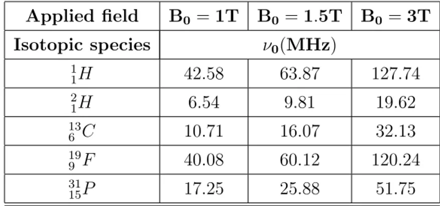
”Larmor frequency”, therefore this expression will be used at times in this thesis when there is no ambiguity. In Table 1.1 the Larmor frequencies ν0 of
different nuclear isotopes used in MR Spectroscopy at various values of B0
Applied field B0 = 1T B0 = 1.5T B0 = 3T Isotopic species ν0(MHz) 1 1H 42.58 63.87 127.74 2 1H 6.54 9.81 19.62 13 6 C 10.71 16.07 32.13 19 9 F 40.08 60.12 120.24 31 15P 17.25 25.88 51.75
Table 1.1: Larmor frequencies of different isotopes at various values of B0.
It is important to mention that, given B0, the nuclei with the higher
intensity in the resonance frequency also provide the more intense NMR signal. Indeed, the advantages of using higher field strength are a linear increase in the signal-to-noise ratio (SNR) and better separation of peaks in the spectrum. More specifically, in clinical applications the most interesting nuclei are1
1H, 136 C and3115P:
• 1
1H-MRS is the more diffuse type of investigation, especially in brain
spectroscopy, mostly because of the natural abundance of protons both in the human body (∼ 62 %) and in organic compounds and also be-cause the proton is the most NMR-sensitive nucleus [2].
• 13
1 C-MRS is interesting in the study of the carbon-containing compound
metabolism (e.g. carbohydrates), even though it occurs at a low aver-age abundance (1,1 %) in relation to the major isotope 12
1 C, which has
a null spin value and therefore is NMR-inactive.
• 31
15P-MRS is important in the analysis of Adenosine TriPhosphate (ATP)
functions and other energetically important metabolites, especially in muscles, and has a moderate NMR-sensitivity.
1.1.3
Chemical shift
Indeed, if all the protons in a mixture of molecules resonated at the same Larmor frequency, magnetic resonance spectra would be limited to a single peak centred on that particular frequency value. However, the resonance fre-quency is highly dependent on the surrounding chemical environment, which is locally variable. In fact, the electronic cloud has a shielding effect on the nucleus, since electrons generate a secondary induced magnetic field which opposes the external field B0. This is because electrons rotate about B0 in
the opposite sense to nucleus spin precession and consequently their magnetic moment µe is aligned against B0, as Figure 1.1 illustrates.
Figure 1.1: Electron shielding of the nucleus.
Therefore, the outcome is that the nucleus senses a magnetic field B0
with reduced intensity because of the shielding given by the electronic cloud. This behaviour, called ”chemical shift”, is expressed as:
Bef f = B0(1 − σ) (1.3)
number (σ < 1), shielding or screening constant, which is dependent on the chemical environment of the nucleus and its relative position within the molecule. Typical values for σ are 10−5 for protons and 10−2 for heavier nuclei. Thus, the frequency at which the nucleus resonates becomes:
νef f =
γ
2πB0(1 − σ) (1.4)
As the equation above indicates, the Larmor precession frequency of the nu-cleus under investigation is slightly displaced. The outcome of the reduction of the magnetic field strength sensed by the nucleus is that the energy differ-ence ∆E of two adjacent Zeeman levels is reduced. Thus, the photon energy required for a transition is lower than in absence of chemical shift.
∆E = −~γBef f (1.5)
Different effective magnetic field will lead to different energies required for the nucleus to flip between Zeeman levels.
It should be outlined that each atom contained in the molecule influ-ences to a certain extent the sensed shielding because it contributes to the overall electronic density. For instance, if the molecule contains one or more electronegative atoms (e.g. Nitrogen, Oxygen, Fluorine, Clorine), the electrons will be pulled away from atoms with less electronegativity (e.g. Hydrogen). Therefore, this resulting electron withdrawal will make the pro-tons deshielded. This phenomenon occurs in molecules in which covalent bonds between atomic electrons are established. A graphical representation can be viewed in Figure 1.2.
The electronegativity of oxygen in the acetaldehyde molecule is such in-tense that it attracts much of the electron cloud. Therefore, protons closer to oxygen are unshielded, while the more distant ones are more shielded [3]. It is common practice not to express chemical shifts in Hertz units since this choice would make chemical shifts dependent on the applied magnetic field strength. Therefore, chemical shift δ are conventionally expressed in
Figure 1.2: Different shielding in the acetaldehyde molecule.
terms of ppm in function of the displacement from the frequency of a refer-ence compound νref measured by the spectrometer [4].
δ(ppm) = ν − νref νref
· 106 (1.6)
Indeed, the reference compound should be chemically inert and the posi-tion of its chemical shift should not fluctuate remarkably because of external variables such as temperature and should produce an evident resonance peak well separated from the other ones. The reference compound is conventionally assigned a 0.00 ppm chemical shift δ. For in vivo applications, compounds whose concentrations do not vary significantly in pathological patients are used. Commonly used reference compounds for different investigations are given in Table 1.2. It is important to underline that in vivo 11H-MRS does not make use of tetramethylsilane, (CH3)4Si, because of its toxicity.
1.1.4
J coupling
A common phenomenon which is observed in spectroscopic analysis is the splitting of resonance peaks into several smaller peaks. This is due to an effect
A
ZX − MRS Reference compound
1
1H − MRS tetramethylsilane (TMS)
in vivo 11H − MRS creatine (Cr)
CH3 peak of N-acetyl aspartate (NAA)
water 13 6 C − MRS tetramethylsilane (TMS) in vivo 31 15P − MRS phosphocreatine (PCr) ATP
Table 1.2: Reference compounds for different MRS investigations.
called ”J coupling” (or ”spin-spin coupling”). The interactions of magnetic moments of the nuclei can occur through space (dipolar coupling) or indi-rectly through electron shared in chemical bonds (scalar coupling). Indeed, even though dipolar interactions between nuclei are important for the relax-ation process in liquids, there is no net contribution to the spectrum thanks to the rapid molecular tumbling which averages these interactions to zero [2]. Meanwhile, overall scalar coupling interactions are not null since they do not depend on the relative distance of the nuclei, but on the intramolecular dis-tance. Therefore, the nearest chemical groups strongly determine the peak displacement observed in the spectrum.
J coupling is established between nuclei with magnetic moments both parallel or antiparallel to the magnetic field and can be homonuclear or het-eronuclear [5]. In addition, scalar coupling is an intramolecular phenomenon since it requires a molecular orbital as a medium for interaction [6]. This characteristic can be exploited to identify the molecular species and their covalent structure.
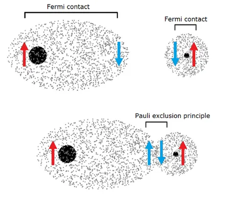
The hyperfine interaction between nuclear and electron spins is governed by the Fermi contact, which energetically favours an antiparallel spin orien-tation. Meanwhile, the Pauli exclusion principle implies that electron spins in the molecular orbital are antiparallel, forcing nuclear and electron spins in
an energetically higher orientation. The relative orientation of spins under J coupling is represented in Figure 1.3.
Figure 1.3: Rearrangement of nuclear and electronic spins through J cou-pling.
As Figure 1.3 displays, one of the two electron spins is parallel to the nuclear spins because of Pauli exclusion principle. This setting leads to an energetically less favourable state.
Because of scalar coupling, a new term must be added to the spin-spin hamiltonian H0, Hscalar:
H = H0+ Hscalar = H0+ 2πJ I1· I2 (1.7)
where J is the coupling constant, which is independent on the applied mag-netic field and is proportional to the proximity of the coupled nuclei. This is an especially interesting feature at high-field MRS since J-coupled multiplets will stay at the same separation, but displaying them in a ppm scale they
will appear closer, thus leading to a more accurate discrimination from the other compounds. Furthermore, the intensity of scalar coupling constants rapidly decrease as the number of bonds increases and can be negligible for more than four bounds [2]. Coupling constant values for chemical bonds commonly found in biomolecules studied in MRS are listed in Table 1.3 [2].
Chemical bond Coupling constant (Hz)
1 1H −11H 1 - 15 1 1H −136 C 100 - 200 1 1H −3115P 10 - 20 13 6 C −136 C 30 - 80 31 15P −168 O −3115P 15 - 20
Table 1.3: Scalar coupling constant values for different chemical bonds.
Taking into account spin-half nuclei for which there are a low energy spin-up state α (m = +12) and a high energy spin-down state β (m = −12), the spin-spin coupling gives rise to four energy levels (αα, αβ, βα, ββ) [7]. The expressions for energies (listed in Table 1.4) depend on the effective resonance frequencies of both nuclei (ωef f,1, ωef f,2) and the correspondent
coupling constant J1,2.
Spin state |m1, m2 > Energy
αα | +1 2, + 1 2 > (− 1 2ωef f,1− 1 2ωef f,2+ 1 4J1,2)~ αβ | +1 2, − 1 2 > (− 1 2ωef f,1+ 1 2ωef f,2− 1 4J1,2)~ βα | − 1 2, + 1 2 > (+ 1 2ωef f,1− 1 2ωef f,2− 1 4J1,2)~ ββ | −1 2, − 1 2 > (+ 1 2ωef f,1+ 1 2ωef f,2+ 1 4J1,2)~
Table 1.4: Energies for a two coupled spin system.
The spectrum of two coupled spins 1, 2 is composed of two doublets each split by the same amount, J1,2, centred at the chemical shift frequencies of
Figure 1.4: Resonance peaks of two coupled spins.
The spectrum shown in Figure 1.4 is a first-order spectrum, which cor-respond to a spin system with |ν2 − ν1| J1,2 and is considered a weakly
coupled spin system. On the other hand, when |ν2− ν1| ∼ J1,2, the system is
strongly coupled, i.e. the αβ and βα states become mixed, and the result is a second-order spectrum. The appearance of the peaks is commonly referred to as the ”roof effect”, which is common in multiplets belonging to the same molecule [7]. This behaviour is represented in Figure 1.5. The inner lines are higher, while the outer are shorter. When the two Larmor frequencies are identical, there is only one peak in the spectrum located at that frequency.
Figure 1.5: Roof effect in strongly-coupled spins. For nuclei with I > 1
rank terms must be taken into account. For instance, the deuteron has I = 1, thus a triplet centred on the effective resonance frequency will be observed in its spectrum.
1.1.5
Nuclear Overhauser effect
According to NMR theory, the strength of a signal is highly dependent on the difference in the Boltzmann level populations. After a perturbating pulse, the magnetization returns back to alignment with B0 through T1 relaxation,
in which nuclei make transitions to reestablish the equilibrium. In uncou-pled spins it may occur that an increase in the signal is observed thanks to a polarization transfer from one nuclear spin population to another saturated one via cross-relaxation. This is known as the ”nuclear Overhauser ef-fect” (nOe). This phenomenon is established through intramolecular dipolar interactions in space, not through chemical bonds as in spin-spin coupling. Therefore, nOe depends on:
• the nature of the nuclei
• the distance between nuclei (the proximity favours dipolar interactions) • the correlation time τC, i.e. the time between two relative
consecu-tive orientations of the dipoles (if it is too long, other effects, such as intermolecular dipolar interactions, will hinder intramolecular dipolar alignment)
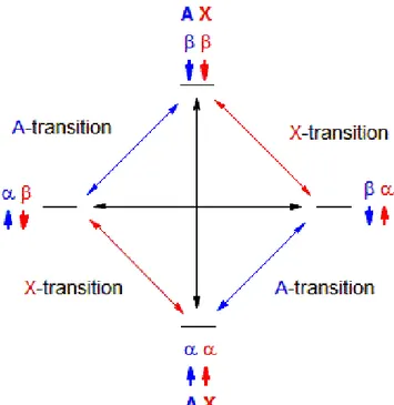
Taking into account two uncoupled nuclei A and X with significant dipolar interaction, there will be four possible combinations of energy levels (Figure 1.6), with αα corresponding to both nuclei in their ground state, αβ and βα representing the cases of only one nucleus in the excited state and ββ being both nuclei in the excited states.
Assuming that αβ and βα are equally populated, at the equilibrium ββ is less populated than αα. If the equilibrium population is altered, the system tends to restore it through relaxation whether by ββ → αα transition, which
Figure 1.6: Energetic level and transition diagram for two uncoupled spins exhibiting nuclear Overhauser effect.
determines a positive nOe for nucleus A (NMR signal enhancement), or by ββ → βα, which implies a negative nOe (NMR signal reduction).
The outcome of positive nOe is an observed increase in the peak ampli-tudes in the spectrum depending on the magnetogyric ratios of nuclei, as expressed the following formula, which is valid for short τC:
η = γX 2γA
(1.8)
where η is the nuclear Overhauser enhancement. This represents a gain factor in the peak amplitude. Values for η under usual in vivo MRS nuclei are reported in Table 1.5 [8].
A-X η
13C −1H 1.3 − 2.9 31P −1H 1.4 − 1.8
Table 1.5: Values for nuclear Overhauser enhancement for typical in vivo MRS nuclei.
1.1.6
Spectrum formation
As it was previously mentioned, in NMR spectroscopy the nuclei do not resonate at the same frequency. Therefore, it is impossible to be on resonance with all the lines in the spectrum since the RF pulse frequency ωRF slightly
differs from the Larmor frequency of the nucleus ω0.
ωRF 6= ω0 (1.9)
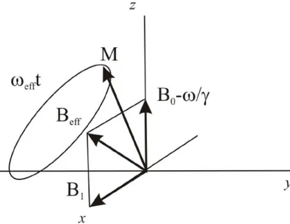
This mismatch implies that the perturbed magnetization in the rotating frame preceeds both around the RF magnetic field B1 and an apparent
mag-netic field Bapp resulting from the imperfect resonance.
Bapp = B0−
ωRF
γ (1.10)
The combination of these two precessions implies that the nuclear spin rotates around an effective field Bef f, as Figure 1.7 displays.
To a certain extent, if the amplitude of B1 is greater than Bapp, we can
assume that the nuclei are on resonance to a first approximation. Therefore, the size of B1 should be as great as the transmitting power of the coils
permits. Such transmitted pulses are referred to as ”hard pulses” and they determine bandwidths up to hundred of kHz. The allowed frequency window is important in MRS because it determines the range of detectable compounds.
In NMR investigations the signal coming from the nuclear magnetization can be detected by perturbating the spin population in the Boltzmann
en-Figure 1.7: Precession of magnetization in the rotating frame when the RF pulse is off-resonant.
ergy level distribution. By applying a 90◦ excitation RF pulse orthogonal to B0, the magnetization vector flips onto the transverse plane. Following
the pulse, the spin precession on the transverse plane induces an oscillatory electromotive force in the receiving coil by electromagnetic induction, orig-inating thus an induced current in the probe. The detected signal is called ”Free induction decay” (FID), which has an oscillating and exponentially decaying trend, as in Figure 1.8 [9], and it is originated by the photons in the radio-wave range emitted by the nuclei returning to the equilibrium.
Mxy(t) = Mxy(0)e − t
T ∗2 (1.11)
The components of the magnetization are: Mx(t) = M0cos[(ω0 − ω)t + φ]e − t T ∗2 My(t) = M0sin[(ω0− ω)t + φ]e − t T ∗2 (1.12)
Figure 1.8: Free induction decay following an excitation pulse.
transverse relaxation because of the inhomogeneities of the magnetic field and to a multi-exponential decay. The detected signal s(t) is proportional to the magnetization.
s(t) = s0eiφeiωte − t
T ∗
2 (1.13)
This signal in the time domain can be represented in the frequency do-main through Fourier transform. The returning FID is a composite signal of many different contributions from metabolites in the volume of interest (VOI), which is resolved into individual resonance frequencies and their rel-ative amplitudes by the Fourier transform.
F (ω) = Z +∞
−∞
s(t)e−iωtdt (1.14)
It is possible to gain a spectrum from one of the two components of the FID, but it is customary to measure both (quadrature detection) to be able to discriminate between positive and negative frequencies in relation to the reference compound. The real and imaginary components of the Fourier transform are:
(
R(ω) = A(ω) cos φ − D(ω) sin φ
I(ω) = A(ω) sin φ + D(ω) cos φ (1.15)
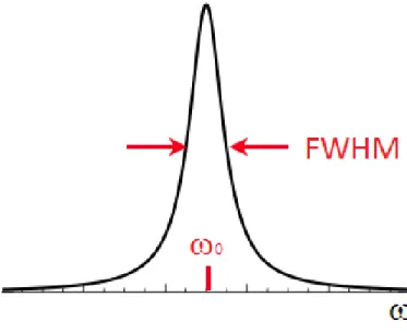
A(ω) = M0T2∗ 1+(ω0−ω)2T2∗2 D(ω) = M0(ω0−ω)T2∗ 2 1+(ω0−ω)2T2∗2 (1.16) A(ω) and D(ω) are the absorption and the dispersion components respec-tively. A(ω) is characterized by a Lorentzian lineshape (Figure 1.9). whose
Figure 1.9: Lorentzian lineshape in the frequency domain. full width at half maximum (FWHM) is:
F W HM = 1 πT2∗ (1.17) where 1 T2∗ = 1 T2 + γ∆B0 (1.18)
∆B0 represents the local field inhomogeneity.
Considering the FWHM of the Lorentzian, it is deducible that the shorter the T∗2 is (i.e. the faster the decay of the FID), the broader the distribution is. This is a major drawback if low-quality scanners with inhomogeneous field are used, where T∗2 is considerably short [5]. The area Σ under the peak (with height hpeak) is:
Σ = π
2F W HM · hpeak (1.19)
The area is proportional to the concentration of the substance resonating at that particular frequency under unsaturated conditions. Since the area under a peak is constant for a given number of nuclei, the peak height decreases with increasing FWHM [3]. Furthermore, if the size of the signal in the time domain increases, the height of the lorentzian curve will be boosted proportionally too. Consequently, it is possible to assess the relative number of nuclei contributing to the signal formation [7].
Actually, a single peak will be observed only in a sample with the same nuclei resonating at the same Larmor frequency. It is more common to notice several peaks in the spectrum. Frequencies which are higher than the value of the reference resonance peak (down-field) are on the left side, whereas lower frequencies (up-field) are on the right, as in Figure 1.10. This convention is due to the fact that more unshielded nuclei give resonance lines at the beginning of the scan. It is customary practice to express the frequencies in ppm or Hertz units and peak heights in arbitrary units. The spectrum and the covalent structure of Lactate, C3H6O3, are given in Figure 1.10 as an
example.
The electronic shielding becomes more prominent reading the spectrum from left to right coherently with the reduction of both the sensed mag-netic field and the resonance frequency. In fact, the methine peak (−CH) is centred on a higher frequency (4.10 ppm) because of the deshielding of the corresponding proton by oxygen atoms, while the three methyl proton peak (−CH3) is located at a lower frequency value (1.31 ppm).
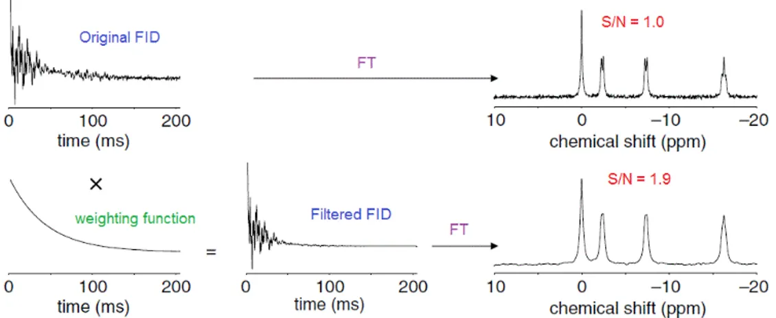
In addition, it should be mentioned that the acquisition of the FID in-evitably records noise in conjunction with the signal from nuclei. This dis-turbance comes from the electronics in the spectrometer, but the major con-tribution is due to thermal noise from the detection coil. At the beginning of the acquisition the signal strength is strongest, but it progressively gets weaker until it is mistakable with noise. To reduce the amount of noise that is
Figure 1.10: Spectrum and covalent structure of Lactate.
present in the signal, the FID is multiplied by a weighting function wSN R(t)
that decreases exponentially with time, suppresses the long tail of the signal curve (where the noise in more intense in relation to the signal) and causes the signal to decay more faster:
wSN R(t) = e−αt (1.20)
where α is a sortable constant value which determines the strength of the decay. As it is displayed in Figure 1.11, the multiplication of the signal for a weighting function evidently reduces the amount of noise both in the acquired FID and the relative spectrum (avoiding an abrupt truncation of the signal, which would lead to artefacts in the spectrum), by almost doubling the signal-to-noise ratio (S/N ).
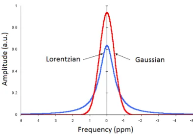
Furthermore, it is common practice to convert the Lorentzian lineshape of peaks to a Gaussian one through the multiplication of the signal for a further weighting function. This method makes peaks more narrow and enhances resolution, as it can be seen in Figure 1.12.
wLG(t) = eβLte−βGt
2
Figure 1.11: Filtering of the FID through weighting function for noise reduc-tion.
where βL and βG are constants required for the lineshape conversion.
However, since resolution enhancement generally results in an increase of noise in a spectrum because of the contribution of the rising exponential [10], optimal outcomes are a compromise which is reached by multiplying the FID with both weighting functions. This overall procedure is called ”apodization” and it is essential in MRS to prevent the spectrum from being too noisy and to enhance the resolution.
s0(t) = s(t)e−αteβLte−βGt2 (1.22)
The FID processing must be preceeded first by a digitization procedure through an Analog-to-Digital Converter (ADC) to enable data to be analyzed and stored in a computer memory. The digitization process samples the signal as a sequence of samples at regular intervals. According to Nyquist-Shannon theorem, in order to avoid aliasing effects, the sampling rate νsampling must
be at least twice as intense as the higher frequency contained in the analog signal as the following expression indicates:
Figure 1.12: Lorentzian and Gaussian resonance lines of equal FWHM and integrated amplitude.
νsampling =
1
∆t > 2νmax (1.23)
where ∆t is the sampling interval. Consequently, the spectral resolution ∆ν is given by:
∆ν = 1
Tacquistion
= 1
N ∆t (1.24)
It is clear that an increase in the acquisition time will lead to a better spectral resolution, although this implies extended data storage and more relative noise. It is customary to lengthen the acquisition time by adding a series of zero amplitude samples after the decay of the FID before applying the Fourier transform. Such a procedure is called ”zero filling” [11].
1.2
Magnetic field gradients in MRI and MRS
1.2.1
Field gradients in MRI
The versatility of NMR tecniques is reflected in the enormous variety of sequences and parameters that are adjustable to retrieve different infor-mation extracted from the detected signal. Generally, both MRI and MRS sequences consist of applications of RF pulses with or without field gradients which have specific durations and timings [12]. Indeed, different types of sequences are characterized by two timing values, echo time TE, which is the time between the 90◦ RF pulse and NMR signal sampling, corresponding to maximum amplitude of echo, and repetition time TR, i.e. the time be-tween two consecutive 90◦ RF excitations pulses, whose duration influences the percentage of longitudinal magnetization recovery.
The signals acquired through MRI scans from each pixel in the image are processed with the aim of discriminating the intrinsic nuclear relaxation properties at different locations in body tissues. This difference in relaxation times leads to different signal intensities, which is explicited in a wide range of contrast in the images, especially in soft tissues. In a simplified expression, the subjective contrast Cs between two points in a T2-weighted image is
determined by the difference in the transverse relaxation times and the echo time TE used in the sequence [13].
Cs ∝ 1 − e − T E
T 0
2−T 002 (1.25)
Another important feature in MRI is space-encoding. The main pur-pose is to make the resonance frequency ω0position-dependent such that after
Fourier transformation different frequencies correspond to different space po-sitions rather than different chemical shift values. This procedure makes use of field gradients by specially designed coils:
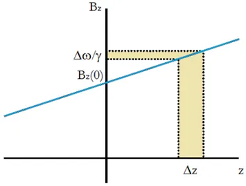
• slice-selective gradients applied along z-axis (at the centre of the bore of the magnet) in concomitance with the RF excitation pulses. Each z position is characterized by a specific resonance frequency ω0(z).
ω0(z) = γ(Bz(0) + Gzz) (1.26)
Therefore, the corrisponding z position is:
z = ω0(z) − γBz(0) γGz
(1.27) Only a selected range of frequencies ∆ω (i.e. positions ∆z) are excited by the RF pulse, as Figure 1.13 displays.
Figure 1.13: Position and frequency ranges excited through slice-selective gradient.
• frequency or read gradients make spins along x-axis resonate ad differ-ent frequencies
• phase gradients make spins along y-axis acquire different phases The latter two gradients are the basis for k-space sampling, which allows the transformation of the selected slice into a raster grid, in which spins belonging to different matrix elements differ whether in frequency or in phase. Mansfield introduced the concept of the space vectors kx and ky, which allow
(
kx = γGxt
ky = γGyt
(1.28) The signal from each location in the mapping relative to a slice with thickness 2a is dependent on the space vector:
s(kx, ky) =
Z a −a
[ Z Z
ρ(x, y, z)ei(kxx+kyy)dxdy]dz (1.29)
The field of view (FOV) in both directions is determined by the gradi-ent intensity and the sampling time (contained in the expressions for space vectors).
(
F OVx= γG2πxt
F OVy = γG2πyt
(1.30) However, the space-encoding procedure basically erases the chemical shift information of nuclei since the spin frequencies are modulated by the gradi-ents (possible residual chemical shifts would be interpreted as noise artifacts), therefore it is not included in the spectroscopic sequences themselves. Indeed, gradients are used in MRS with different purposes.
1.2.2
Field gradients in MRS
The main concerns in MRS are the acquisition of the spectrum with a lineshape as well-resolved and not distorted as it can be achieved and the spatial assignment of the detected signal which is generally accomplished through a MRI acquisition prior to the MRS sequence. Actually, there are two types of localization procedures (single- or multi-voxel techniques), which will be discussed in detail in later sections.
Spectroscopic sequences generally use slice-selective RF pulses with orthogonal field gradients in order to define the volume of interest from the intersection of the excited slices, thus restricting the signal detection to a specific region (spatial localization).
In addition, MRS sequences make use of field gradients as a means to suppress unwanted signals and to guarantee a more homogeneous field in the area of interest. These are called ”crusher or spoiler gradients”, which dephase the transverse component of the magnetization such that coherences and consequently the signal are cancelled. However, the effects of gradients can be partially reversed by the application of a subsequent gradient which undoes the dephasing. Since dephasing proceeds at a different rate for dif-ferent spins, gradient pulses of difdif-ferent strengths and durations are applied to restore most of the overall coherence.
The outcome of the switch of gradients during the MRS acquisition is a net enhancement in spatial resolution. These matters are of the utmost importance for in vivo characterizations, since they allow an accurate exam-ination of a tissue of interest without the signal contamexam-ination from other tissues.
Ideal magnetic field homogeneity is a condition which is difficult to achieve since the static field is inherently nonuniform because of design con-straints of the magnet. However, it is considered a fundamental parameter to assess the quality of the magnet in use and is more crucial in spectroscopic rather than imaging investigations since poor field homogeneity results in both a lower SNR and broadening of the width of the peaks. Frequently the inhomogeneity ι of two systems (often expressed in ppm units) is estimated by measuring the ratio of the maximum fluctuation measured in a specific spherical volume (e.g. corresponding to the volume of a dedicated spherical phantom) and the nominal value of the static field.
ι(ppm) = ∆B0 B0
· 106 (1.31)
Indeed, a fundamental preliminary procedure in MRS is shimming, which is the adjustment of field gradients to optimize the magnetic homo-geneity over the volume of interest (VOI). This is accomplished through reg-ulation of currents in dedicated gradient coils. Fluctuations in the magnetic field cause line broadening and distortions in the spectrum together with
reduced SNR. In particular, this procedure becomes more relevant at higher fields where good local shimming prevents peaks from overlapping, in spite of the increase in sensitivity. Indeed, a major problem in high-field MRS is that T∗2 relaxation times become shorter because of the greater magnetic susceptibilities, especially when sequences are applied in vivo [15]. When a magnetic field is applied, small magnetic field gradients are originated be-tween tissue interfaces with different values of susceptibility. These local gradients enhance the dephasing between spins, thus degrading the spectral resolution. This setback is reduced thanks to improved shimming systems [16].
Furthermore, the field homogeneity is also needed to reduce signal con-taminations from the surroundings, a problem known as ”voxel bleed” [12]. This effect is due to displacements in the slice selection for compounds with different relative chemical shifts or imperfect slice-selective pulses. In ad-dition, the excited VOI should be as sharp as possible in the edges. It is common practice to perform an imaging sequence prior to the spectrum acquisition in order to correctly identify the VOI. Figure 1.14 depicts the relative displacement of the fat and water voxels.
Figure 1.14: Fat voxel offset location with respect to the water voxel.
Another matter of concern is represented by eddy currents ieddy(t) which
are induced in the magnet by the variation of the magnetic flux of fluctuating fields (e.g. switching on gradient pulses), as Faraday’s law states:
ieddy(t) = −
1 R
∂Φ(Beddy)
∂t (1.32)
where R is the electrical resistance of the medium and Φ(Beddy) is the
mag-netic flux.
Since these parasite currents cause further distortions in the peak shapes and signal dephasing and they can last for hundreds of milliseconds, it is essential that electronic hardware is unaffected by low levels of eddy currents especially when sequences with short TEs are applied [17]. This is due to the fact that eddy currents with time constants comparable to echo times are difficult to differentiate from the actual signal currents [18].
The reduction of these effects is achieved by applying corrective currents in the gradient coils whose amplitudes and decay characteristics are set in order to offset the eddy currents [19] by a phase factor ∆φ(r). For instance, after a 90◦ pulse followed by a gradient the phase of these currents must be adjusted according to the amplitude of the gradient and the echo time. Another technological advance is represented by shielded gradient coils, which do not produce significant magnetic fields outside the sample volume and minimize the generation of eddy currents. They are composed of an inner main coil and an outer shield coil connected in series together with cooling cladding. The outer coil produces a field which opposes the one from the inner coil with such amplitude that net field outside the coils (fringe field), which creates disturbances and is useless for experiments, is almost null, leading to reduced effects of eddy currents [20].
∆φ(r) ∝ γ[B0+ G(t)r]T E (1.33)
In conclusion, it should be mentioned that the introduction of many field gradients into the spectroscopic sequences inevitably determines a delay be-tween the application of RF pulses and the signal recording by the receiver. This is the reason why sequence developers aim to reach a balance between sequence timing values and the expected outcomes.
1.3
Single-volume localization sequences
1.3.1
Selective pulses and relaxation times
All single-volume localization sequences consist essentially of the selection of a spatially selective slice by the application of frequency-selective RF pulses in conjunction with B0 magnetic field gradients. The final outcome is the
investigation of the signal from one volume at a time [21]. Usually the VOI is defined by the intersection of three orthogonal slices selected by three applied RF pulses, as represented in Figure 1.15. For instance, a typical VOI size for brain spectroscopy is 8 cm3.
Figure 1.15: Defined VOI from intersection of the three slice-selective RF pulses applied in orthogonal directions.
The contribution of magnetization from spins outside the VOI must be suppressed as efficiently as possible by using pulses with good excitation profile and crusher gradients. There are several combinations of RF pulses and fields gradients which may be chosen to select a 3D volume. The VOI is previously selected through a MRI scan (”image-guided spectroscopy”). Anyway, it is important to be aware that the results of the application of
different sequences lead to different parameters in the spectra, therefore a critical spectral analysis requires an accurate discussion of the most com-monly used acquisition methods (ISIS, STEAM and PRESS).
Furthermore, it is worth to mention that MRS sequences must avoid in-fluences of relaxation times on signal intensity. This is because the NMR signal is proportional to concentrations only if T1 saturation and T2 decay
effects are negligible [3]. To avoid T1 saturation of the compounds of
inter-est, the repetition time for the acquisition should be 5 times greater than the longitudinal relaxation time. However, for clinical purposes scans are repeated after:
T R > 3T1 (1.34)
In clinical studies shorter TR values are commonly used in practice and partial saturation is consented not to increase the total acquisition time (es-pecially in clinical routines). Effects due to T2 relaxation are more evident
if long-TE sequences are used, nevertheless short-TE sequences have become more diffuse.
1.3.2
ISIS
The ISIS sequence (Image Selected In vivo Spectroscopy) leads to a com-plete 3D volume localization in eight scans [22]. Basically, it consists of three frequency-selective on/off 180◦ pulses in concomitance with three orthogo-nal magnetic field gradients, followed by a 90◦ pulse, which originates the acquired FID. The pulse sequence for ISIS is depicted in Figure 1.16.
After zero or an even number of 180◦ pulses, the magnetization ends up along the positive longitudinal axis and flips onto the positive y axis thanks to a 90◦pulse, whereas after an odd number of 180◦pulses, the magnetization is aligned with the negative longitudinal axis and is excited to the negative y axis by a 90◦ pulse [2]. Inversion 180◦pulses are switched on or off depending on the current acquisition scan Si (i = 1, ...8), as represented in Table 1.6.
Figure 1.16: Pulse sequence for ISIS.
The volume selection is based on the sum and subtraction of the scans Si to accumulate the signal in the desired VOI and erase the signal coming
from other locations.
SV OI = S1− S2− S3+ S4− S5+ S6+ S7− S8 (1.35)
However, ISIS is a sequence whose accuracy is poor because it is highly sensitive to movements of the sample under investigation, which may lead to displacements of the VOI and thus artifacts due to signal contamination. The algebraic operations on the acquired scan would lead to systematic errors. In addition, the more inhomogeneous the magnetic field is, the lower the signal intensity is. Although ISIS is frequently used in the investigations of short T2 species, transverse relaxation during 180◦ pulse may cause further
degradation in the localization. Therefore, an accurate shimming is difficult because of the number of scans.
Another major setback in ISIS is the so-called ”T1 smearing”, which
causes further signal loss. This inconvenience occurs when the longitudinal relaxation is incomplete between two of the eight subsequent scans [23]. The
Scan 1st 180◦ pulse 2nd 180◦ pulse 3rd 180◦ pulse
S1 off off off
S2 on off on S3 off on off S4 on on off S5 off off on S6 on off on S7 off on on S8 on on on
Table 1.6: Switching of the inversion pulses in ISIS scans.
amplitude of the longitudinal magnetization is progressively reduced as the scans are acquired and the cancellation of the unwanted signals is incom-plete. T1 smearing is dependent on the field inhomogeneity and the repetion
time duration relative to T1 relaxation time. However, T1 smearing can be
contained if signal averaging of each individual ISIS scan is performed.
1.3.3
STEAM
STEAM (STimulated Echo Acquisition Mode) is a single-shot localization sequence. The basic pulse sequence (Figure 1.17) consists of three 90◦ RF pulses together with field gradients, a combination which originates three FIDs, four spin echoes (SE) and a stimulated echo (STE), which is the one that is recorded. Since only 90◦ pulses, which have shorter duration than 180◦ pulses, are applied in this sequence, STEAM is the first choice when short TEs are needed. Short TEs (< 40 ms) permit a reduced signal loss and therefore high SNR, which allows the observation of some peaks that would not be detected at longer TEs, but on the other hand the noise is enhanced too.
Figure 1.17: Pulse sequence for STEAM.
time (TM), a period during which magnetization transfer between the spin system is allowed through nOe cross-relaxation. As it can be viewed in Figure 1.17, the stimulated echo is formed after a TE + TM delay (or after TE/2 following the last 90◦ pulse). During TE period the magnetization is mainly affected by T2 relaxation, whereas T1 relaxation is prevailing in the TM
period. Indeed, since the magnetization is not influenced by T2 relaxation
during TM, STEAM is frequently used for the analysis of species with short T2 values and relatively long T1 values.
It is important that STE be successfully isolated from SEs and FIDs. This is accomplished in two ways:
• phase cycling, i.e. the phases of the pulses and the receiver are sys-tematically varied in order to cancel unwanted signals. This procedure is generally avoided since it requires to be applied iteratively, although STEAM is a single-scan method. However it can be used if scans are repeated to increase SNR.
• switch of crusher field gradients for a short period of time to dephase FIDs and SEs. This choice does not require repetition.
Mxy =
1
2M0sin θ1sin θ2sin θ3e
−T M T1 e− T E T2e− 16 π2γ 2G2δ2(∆−δ 4)D (1.36)
where θi (i = 1, 2, 3) represents the nutation angle of RF pulse i, G is the
amplitude of the gradient, ∆ is the delay between two gradients in the two TE/2 periods, δ is their duration and D is the diffusion coefficient. As the equation above indicates, the amplitude of a STE is expected to be half of the equilibrium magnetization M0, notwithstanding relaxation and diffusion
effects. This is because the second 90◦ pulse only rotates half of the trasverse magnetization to the longitudinal plane, while the other one is dephased by a crusher gradient switched during TM duration. Consequently, this method implies a decreased SNR by a factor of 2 in relation to equilibrium magne-tization (and PRESS sequence too, as it will be discussed in the following section) [5].
Actually, diffusion processes are disadvantageous for MRS investigations because if spins are given too much time between RF pulses, there will be an evident decrease in the amplitude of the magnetization and the SNR will drop. Therefore, echo times shorter than 30 ms are generally preferred in clinical STEAM. Even TE values from 1 to 6 ms have been used in research studies with faster excitation pulses and crusher gradients at ultra-high fields [24], even though there is incomplete magnetization recovery and overlapping of peaks is more pronounced [1].
1.3.4
PRESS
PRESS (Point RESolved Spectroscopy) is a single-scan sequence primar-ily composed of a 90◦ pulse followed by two refocusing 180◦ pulses, as repre-sented in Figure 1.18. Therefore, the method is characterized by the forma-tion of two spin echoes. The 90◦ pulse selects the plane of interest. Following the first 180◦ pulse the first echo forms after a delay TE1 and contains signal
from a column resulting from the intersection of two planes selected by both the 90◦and the 180◦ pulses. The successive refocusing occurs during a delay
TE2, such that the final echo forms at the following echo time:
T E = T E1+ T E2 (1.37)
Figure 1.18: Pulse sequence for PRESS.
This echo only contains signal from the intersection of the three selected planes, i.e. precisely the volume of interest, depicted in Figure 1.19. Indeed, signal from outside the VOI is not excited and rapidly dephased by crusher gradients. Even the first echo needs to be dephased for the acquisition to be successful. If outer signal is recorded, this disturbance is due to incomplete removal of coherences, magnetic field inhomogeneities or partial suppression of other prevailing signals, as it will be discussed in the following section. All these matters of concern influence the spectral quality.
More scan accumulations are needed in order to gain a sufficient SNR (ordinarily 8 or 16 are sufficient) and reduce possible artifacts by sum of the detected signals. However, it should be stressed that PRESS is charac-terized by a SNR value approximately higher than STEAM by a factor of 2. This is the reason why PRESS is the most frequently used localization technique. Anyway, STEAM is a preferable sequence choice when short TEs are needed since PRESS requires inevitably longer TE values because of the longer duration of the 180◦ pulses [21]. When the first MRS scanners were
Figure 1.19: Spatial localization by PRESS pulses.
developed, the lower boundary for TEs in PRESS was 144 ms, but nowadays it is possible to reach even values of about 30 ms [12].
In addition, PRESS tends to underestimate T2 values of some molecules,
especially if long TEs are used [25]. This effect is due to J coupling inter-actions which accelerate the signal decay and enhance spin dephasing. The consequent outcome is the broadening of the spectral peaks. STEAM seems to be more insensitive to this drawback because of the shorter TEs, although it is affected anyway by such effect [26].
1.3.5
Imperfect RF pulses
The ideal result of any localization technique would be a perfectly sharp edge of the excited VOI, since it is evidence of high localization accuracy and volume definition. Anyway, it is a more realistic assumption that the selected VOI will be slightly smeared because of the finite length of the applied pulses. Each RF pulses is characterized by its excitation profile, i.e. its Fourier transform, which also includes a transition frequency range in which the flip angle between 0◦ and 90◦ or 180◦ of the magnetization is included. This
inherent imperfection in the applied pulses causes smoothness in the edge profile and contamination from the outer areas.
The application of STEAM leads to a more definite volume profile than PRESS because 90◦ pulses are generally produced with a sharper excita-tion profile. Therefore, STEAM is recommended for brain MRS applicaexcita-tions where contamination from surroundings is to be avoided [21].
1.3.6
Signal suppression methods
Some compounds such as water and fat are found in greater abundance than others in human tissues and consequently the proton MRS spectrum is dominated by the higher signals originated by hydrogens contained in these molecules. Generally, the concentrations of metabolites are lower than those of water by more than 4 orders of magnitude. Typical metabolites concentrations are in the millimolar range (1 − 10mM), while water molar concentration is in the order of tens of molar concentrations [27]. The latest electronic acquisition systems are able to record the low metabolite peaks despite the greater amplitude of the water resonance. Anyway, the presence of such an overshot peak in the acquired spectrum might lead to baseline distortions and contaminated signals compromising a reliable detection of metabolite [28].
To overcome this difficulty and remove baseline alterations, suppression of water and/or fat signals is frequently performed. The removal of particular resonances in the spectrum is only allowed if the compound that is interfer-ing with the detection possesses a property which discerns it from the other molecules (whether it may be chemical shift, scalar coupling, or T1 or T2
relaxation times). An additional benefit from the signal suppression is the reduction of the dynamic range, i.e. the ratio between the largest and small-est signal values that must be processed by the electronic systems, since the difference of the highest and the lowest NMR signal detected by the receiver is smaller. Anyway, this is not an overriding concern with recent electronic hardware.