Human-Driven FOL Explanations of Deep Learning
Gabriele Ciravegna
1,2, Francesco Giannini
2, Marco Gori
2,3Marco Maggini
2and Stefano Melacci
2∗1
Department of Information Engineering, University of Florence, Florence, Italy
2
SAILab, Department of Information Engineering and Mathematics, University of Siena, Siena, Italy
3Maasai, Universit`e Cˆote d’Azur, Nice, France
[email protected],{fgiannini,mela,maggini,marco}@diism.unisi.it
Abstract
Deep neural networks are usually considered black-boxes due to their complex internal architec-ture, that cannot straightforwardly provide human-understandable explanations on how they behave. Indeed, Deep Learning is still viewed with skepti-cism in those real-world domains in which incor-rect predictions may produce critical effects. This is one of the reasons why in the last few years Ex-plainable Artificial Intelligence (XAI) techniques have gained a lot of attention in the scientific com-munity. In this paper, we focus on the case of multi-label classification, proposing a neural network that learns the relationships among the predictors as-sociated to each class, yielding First-Order Logic (FOL)-based descriptions. Both the explanation-related network and the classification-explanation-related net-work are jointly learned, thus implicitly introduc-ing a latent dependency between the development of the explanation mechanism and the develop-ment of the classifiers. Our model can integrate human-driven preferences that guide the learning-to-explain process, and it is presented in a unified framework. Different typologies of explanations are evaluated in distinct experiments, showing that the proposed approach discovers new knowledge and can improve the classifier performance.
1
Introduction
In the last few years the scientific community devoted a lot of effort to the proposal of approaches that yield ex-planations to the decisions of machine learning-based sys-tems [Bibal and Fr´enay, 2016; Doshi-Velez and Kim, 2017; Doˇsilovi´c et al., 2018; Guidotti et al., 2018; Teso and Ker-sting, 2019]. In particular, several Explainable Artificial In-telligence (XAI) [Gunning, 2017] techniques have been de-veloped, with different properties and output formats. They generally rely on existing interpretable models, such as de-cision trees, rules, linear models [Freitas, 2014; Huysmans et al., 2011], that are considered easily understandable by
∗
Contact Author
humans. On the other hand, in order to provide an ex-planation for black-box predictors, such as (deep) neural networks and support vector machines, a new interpretable model that is as faithful as possible to the original predictor is considered, sometimes acting on localized regions of the space [Guidotti et al., 2018]. Then, the explanation prob-lem consists in finding the best interpretable model approx-imating the black-box predictor. In the context of the XAI literature, there is no clear agreement on what an explana-tion should be, nor on what are the suitable methodologies to quantitatively evaluate its quality [Carvalho et al., 2019; Molnar, 2019]. There is also a strong dependence on the tar-get of the explanation, e.g., a common user, an expert, or an artificial intelligence researcher.
In this paper, we consider multi-label classification, where each input example belongs to one of more classes, and on First-Order Logic (FOL)-based explanations of the behaviour of the classifier. We focus on neural network-based sys-tems, that implicitly learn from supervisions the relationships among the considered classes. We propose to introduce an-other neural network that operates in the output space of the classifier, also referred to as concept space, further project-ing the data onto the so-called rule space, where each co-ordinate represents the activation of a rule/explanation that, afterwards, is described by FOL. In particular, we propose to progressively prune the connections of the newly intro-duced network and interpret each of its neurons as a learn-able boolean function (an idea related to several methods [Fu, 1991; Towell and Shavlik, 1993; Tsukimoto, 2000; Sato and Tsukimoto, 2001; Zilke et al., 2016]), ending up in a FOL formula for each coordinate of the rule space.
The concepts-to-rules projection can be learned using dif-ferent criteria, that bias the type of rules discovered by the system. We propose a general unsupervised criterion based on information principles, following [Melacci and Gori, 2012]. However, humans usually have expectations on the kind of explanations they might get. For example, suppose we are training a network to classify digits and also to predict whether they are even numbers. If we do not know what being evenmeans, we might be particularly interested in knowing the relationships between the class even and the other classes (i.e., that even numbers are 0 or 2 or 4 or 6 or 8). It could not be so useful to discover that 0 is not 2, even if it is still a valid explanation in the considered multi-label problem.
Mo-tivated by this consideration, we propose a generic framework that can discover both unbiased and user-biased explanations. A key feature of the proposed framework is that learning the classifier and the explanation-related network takes place in a joint process, differently from what could be done, for example, by classic data mining tools [Liu, 2007; Witten and Frank, 2005]. This implicitly introduces a latent dependency between the development of the explanation mechanism and the one of the classifiers. When cast into the semi-supervised learning setting, we show that linking the two networks can lead to better quality classifiers, bridging the predictions on the unsupervised portion of the training data by means of the explanation net, that acts as a special regularizer.
The paper is organized as follows. Section 2 introduces the use cases covered in this paper, while the proposed model is described in Section 3. Experiments are collected in Section 4 and Section 5 concludes the paper.
2
Scenarios
We consider a multi-label classification problem, in which a multi-output classifier is learned from data. Each output unit is associated to a function in [0, 1] that predicts how strongly an input example belongs to the considered class. We will also interchangeably refer to these functions as task functions (in a more general perspective where each function is related to a different task), or predicates (if we interpret each output score as the truth value of a logic predicate).
We also consider a set of explanations, that express knowl-edge on the relationships among the task functions, and that are the outcome of the proposed approach. Such knowledge is not known in advance, and it represents a way to explain what the classifier implicitly learned about the task functions. In order to guide the process of building the explanations, the user can specify one or more preferences. In particular, the user can decide if the explanations have to describe lo-cal relationships that only hold in sub-portions of the concept space or global rules that hold everywhere, or even if they must focus on a user-selected task function (as in the exam-ple of Section 1). In what follows we report an overview of the specific use cases explored in this paper.
Local Explanations. In this scenario, the explanations are automatically produced without making any assumptions on which task functions to consider. In order to provide a valid criterion to develop explanations, we enforce them to only hold in sub-portions of the concept space and, overall, to cover the whole dataset. The user can provide an example to the trained network and get back the explanation associated to it, that may highlight partial co-occurrences of the task func-tions. For instance, the system might discover that “eyes or sunglasses” is a valid rule for some pictures (the ones with faces) but not for others (the ones without faces).
Global Explanations. Local explanations may provide very specific knowledge concerning only small portions of data. In order to describe more general properties that hold on the whole dataset, we may be interested in global explana-tions. Global explanations may catch general relations among task functions that are valid for all the points of the considered
dataset, such as mutual exclusion of two classes or hierarchi-cal relations.
Class-driven Explanations. The user may require explana-tions about the behaviour of specific task funcexplana-tions. He could also specify if he is looking for necessary conditions (IF →) or necessary and sufficient explanations (IFF ↔). For in-stance, focusing on the driving class man, we may discover that a certain pattern is classified as “man only if it is also classified as containing hand, body, head”, and so on. In the example of Section 1, even was the class driving a necessary and sufficient explanation. The rules of this scenario are com-pletely tailored around the user-selected target classes. Combined Explanations. All the scenarios described so far may be arbitrarily combined in case the user is simulta-neously interested in multiple explanations according to dif-ferent criteria. In particular, some explanations might have to specify the behaviour of some task functions, while the remaining ones might have to be automatically acquired in order to describe global or local interactions.
3
Model
We consider data belonging to the perceptual space X ⊆ Rd, and n labels/classes, each of them associated to a task func-tionfi, i = 1, . . . , n, that corresponds to an output unit of a
neural network. For any x ∈ X, fi(x) ∈ [0, 1] expresses the
membership degree of the example x to the i-th class. We in-dicate with f (x) the function that returns the n-dimensional vector with the outputs of all the task functions. Such vector belongs to the so-called concept space.
Let us consider another set of functions implemented by neural networks, indicated with ψj, j = 1, . . . , m, whose
input domain is the concept space while their output domain is the rule space. Each ψj(f (x)) expresses the validity of
a certain explanation with respect to the output of the task functions on the data sample x ∈ X. In addition, we assume ψj(f (x)) ∈ [0, 1] in order to relate the value of ψj to the
truth-degree of a certain FOL formula.
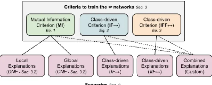
Different criteria are needed to learn the parameters of the functions ψj in order to implement the scenarios of
Sec-tion 2, as we will describe in SecSec-tion 3.1. Once the ex-plaining functions are learnt, we will consider their approx-imation as boolean functions, and they will be given a de-scription in terms of FOL, as we will discuss in Section 3.2. Throughout the paper, the notation ˆψj denotes both the
ap-proximating boolean function and its associated logical for-mula. Finally, Xjdenotes the subset of the input space where
the j-th explanation holds true, also named its support, i.e., Xj = {x ∈ X : ˆψj(f (x)) = 1}. When no subscript is
spec-ified, f and ψ indicate the collection of all the fi’s and ψj’s,
respectively.
3.1
Learning Criteria
We consider a semi-supervised setting in which only a portion of the data in X is labeled [Melacci and Belkin, 2011]. This is a natural setting of several real-world applications, since getting labeled data is usually costly, and it also allows us
to better emphasize the proprieties of the explanation learn-ing mechanisms, that can exploit both labeled and unlabeled training data with no distinctions.
The classic cross-entropy loss is used to enforce the task functions fi’s to fit the available supervisions, paired with
a regularization criterion to favour smooth solutions (weight decay). In order to implement the scenarios of Section 2, we need to augment the training loss with further criteria (penalty terms) that involve the explaining functions ψj’s, for all x’s,
being them labeled or not, and described in what follows.1 Mutual Information-based Criterion. The maximization of the Mutual Information (MI) between the concept and rule spaces can be enforced in order to implement the principles behind the Local Explanations scenario, and it could also be used as a basic block to implement the Global Explanations scenario (Section 2). In the latter case, further operations are needed, and they will be described in Section 3.2. Maximiz-ing the transfer of information from the n task functions to the m explaining functions is a fully unsupervised process that leads to configurations of the ψj’s functions such that,
for each x ∈ X, only one of them is active (close to 1) while all the others are close to zero (see [Melacci and Gori, 2012]). In order to define the MI index, we introduce the probability distribution PΨ=j|Y =f (x)(ψ, f (x)), for all j, as the
probabil-ity of ψj to be active in f (x). Following the classic notation
of discrete MI, Ψ is a discrete random variable associated to the set of explaining functions while Y is the variable related to the data in the concept space.2 The penalty term to
mini-mize is minus the MI index, that is
LM I(ψ, f, X) = −HΨ(ψ, f, X) + HΨ|Y(ψ, f, X) , (1)
where HΨ and HΨ|Y denote the entropy and conditional
entropy functions (respectively) associated to the aforemen-tioned probability distribution and measured over the whole X. An outcome of the maximization of the MI index is that the supports of the explaining functions will tend to partition the input space X, i.e., X = Sm
j=1Xj and
Xj ∩ Xk = ∅, for j 6= k (see [Melacci and Gori, 2012;
Betti et al., 2019] for further details).
Class-driven Criteria. The Class-driven Explanations sce-nario of Section 2 aims at providing explanations for user-selected task functions. Let assume that the user wants the system to learn an explaining function ψh(i)that is driven by
the user-selected fi, being h(·) an index mapping function.
We propose to enforce the support Xh(i)of ψh(i)to contain
(IF →) or to be equal to (IFF ↔) the space regions in which fiis active. Notice that fiand ψh(i)have different input
do-mains (perceptual space and concept space, respectively), so we are introducing a constraint between two different repre-sentations of the data (see e.g. [Melacci et al., 2009]). More-over, since the goal of this scenario is to explain fiin terms
of the other fu6=i’s, we mask the i-th component of f (x) by
setting it to 0 for all x ∈ X. This also avoids trivial so-lutions in which ψh(i) only depends on fi. We denote by
1
Each penalty term is intended to be weighed by a positive scalar. 2
We implemented the probability distribution using the softmax operator, scaling the logits with a constant factor to ensure that when ψj(x) = 1 all the other ψz6=j0 are zero.
Mutual Information Criterion (MI) Eq. 1 Class-driven Criterion (IF→) Eq. 2 Class-driven Criterion (IFF↔) Eq. 3
Criteria to train the ᴪ networks Sec. 3
Local Explanations (DNF - Sec. 3.2) Global Explanations (CNF - Sec. 3.2) Class-driven Explanations (IF→) Class-driven Explanations (IIF↔) Scenarios Sec. 2 Combined Explanations (Custom)
Figure 1: The criteria of the proposed framework and their relations with the use-cases of Section 2.
P, S ⊆ {1, . . . , n} the disjoint sets of task function indexes selected for class-driven IF → and IFF ↔ explanations, re-spectively. The loss terms that implement the described prin-ciples are reported in Eq. 2 and Eq. 3,
L→(ψ, f, X) = X i∈P,x∈X max{0, fi(x) − ψh(i)(f (x))} (2) L↔(ψ, f, X) = X i∈S,x∈X |fi(x) − ψh(i)(f (x))| . (3)
While Eq. 2 does not penalize those points on which ψh(i)(x) > fi(x), Eq. 3 specifically enforces the ψh(i)and
fito be equivalent. In order to avoid trivial solutions of Eq.
2 in which, for instance, ψh(i)is always 1, we enforce the
su-perivision loss of fi also on the output of ψh(i). Notice that
these losses never explicitly estimate Xh(i).
Class-driven & Mutual Information-based Criteria. The Combined Explanationsscenario of Section 2 is the most gen-eral one, and it can be implemented involving all the penalty terms described so far. The MI index can be enforced only on those ψj’s for which the user is looking for a local
ex-planation, while other explaining functions can be dedicated to class-driven explanations. Interestingly, we can also nest the MI index inside a class-driven explanation, since the user could ask for multiple local explanations for each selected driving class. In this case, multiple ψj’s are allocated for
each driving class, and the MI index is computed assuming the probability distribution of the discrete samples in the con-cept space to be proportional to the activation of the task func-tion we have to explain. This scenario can be arbitrarily made more complex, and it is out of the scope of this paper to focus on all the possible combinations of the proposed criteria.
Fig. 1 summarizes the role of the described loss terms and their relations with the scenarios of Section 2.
3.2
First-Order Logic Formulas
Each explaining function ψj is a [0, 1]-valued function
de-fined in [0, 1]n. At the end of the training stage, each ψ j
is converted into a boolean function ˆψj (this is also
con-sidered with a different goal e.g. in [Fu, 1991; Towell and Shavlik, 1993; Tsukimoto, 2000; Sato and Tsukimoto, 2001; Zilke et al., 2016]), and then converted into a FOL formula.
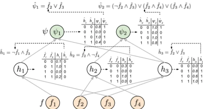
The booleanization step is obtained by approximating any neuron output with its closest integer (assuming sigmoids as activation functions, this value can only be 0 or 1) and by re-peating this process for each layer, from the output neurons of the task functions up to the output layer of ψ. As a result,
h1 h3 ψ1ψ1 0 0 0.8 1 0 1 0.0 0 1 0 1.0 1 1 1 0.4 0 h2 h3 ψ2ψ2 0 0 1.0 1 0 1 0.0 0 1 0 1.0 1 1 1 0.8 1 f1 f3 h1 h1 0 0 0.1 0 0 1 1.0 1 1 0 0.0 0 1 1 0.2 0 f2 f4 h2 h2 0 0 0.3 0 0 1 0.0 0 1 0 1.0 1 1 1 0.0 0 f2 f3 h3.h3 0 0 0.0 0 0 1 0.8 1 1 0 0.6 1 1 1 1.0 1 ^ ^ ^ ^ ^ ^ ^ ^ ^ ^ ^ ^ ^ ^ ^
Figure 2: Extracting FOL formulas from each ψj. Hidden and out-put neurons are paired truth tables (right) and their corresponding logic description (top), as described in Sec. 3.2. The truth tables in-clude the real-value neuron outputs (third column) and their boolean approximation (last column). The FOL descriptions of ψ1, ψ2 are the outcome of composing the truth tables of the hidden neurons.
for each neuron we get a boolean function, whose truth-table can be easily rewritten as a boolean formula in Disjunctive Normal Form (DNF), i.e., a disjunction of minterms (con-junction of literals). By composing the formulas attached to each neuron, accordingly to the network structure, we get ˆψj,
that is the boolean formula of the output neuron associated to ψj. The whole procedure is illustrated in the example of
Figure 2. Clearly, this procedure is efficient only if the fan-in of each neuron is small, a condition that we enforce with the procedure described in Section 3.3.
In the case of Local Explanations (Section 2), each ψj is
close to 1 only in some sup-portions of the space, due to the maximum mutual information criterion, so that the FOL rule
ˆ
ψjwill hold true only on Xj ⊂ X (and false otherwise). As
a consequence, each explanation is local,
∀x ∈ Xj, ˆψj(f (x)) , for j = 1, . . . , m .
The case of Global Explanations (Section 2) is still built on the maximum mutual information criterion. A global ex-planation (i.e., an exex-planation holding on the whole input space X) can be obtained by a disjunction of ˆψ1, . . . , ˆψm.
However, the resulting formula will be generally unclear and quite complex. A possible approach to get a set of global explanations starting from the previous case is then to con-vert it in Conjunctive Normal Form (CNF), i.e., a conjunc-tion of K disjuncconjunc-tions of literals { ˆψk0, k = 1, . . . , K}, Wm
j=1ψˆj(f (x)) ≡ V K
k=1ψˆ0k(f (x)). In this case, the
follow-ing global formulas are valid in all X,
∀x ∈ X, ˆψk0(f (x)) , for k = 1, . . . , K . (4) Unfortunately, converting a boolean formula into CNF can lead to an exponential explosion of the formula. However, after having converted each ˆψjin CNF, the conversion can be
computed in polynomial time with respect to the number of minterms in each ˆψj[Russell and Norvig, 2016].
The Class-driven Explanations (Section 2) naturally gen-erate rules that hold for all X but that are specific for some set of predicates. In particular, Eq. 2 and Eq. 3 enforce 1fi ⊆ Xh(i)and 1fi = Xh(i)respectively (for all i ∈ P and
i ∈ S), being 1fi the characteristic function associated to
re-gions where fiis active. From a logic point of view, we get
the validity of the following FOL formulas: ∀x ∈ X, ˆfi(x) → ˆψh(i)(x) for i ∈ P ,
∀x ∈ X, ˆfi(x) ↔ ˆψh(i)(x) for i ∈ S ,
where → and ↔ are the implication and logical equivalence, respectively, and ˆfiis the boolean approximation of fi.
3.3
Learning Strategies
Keeping the fan-in of each neuron in the ψ-networks close to small values is a condition that is needed in order to effi-ciently devise FOL formulas. L1-norm-based regularization
can be exploited to reduce the number of non-zero-weighed input connections of each neuron. After the training stage, we propose to progressively prune the connections with the smallest absolute values of the associated weights, in order to keep exactly q ≥ 2 input connections per neuron. This pro-cess is performed in an iterative fashion. At each iteration, only one connection per neuron is removed, and a few op-timization epochs are performed (using the same loss of the training stage), to let the weights of the ψ functions to re-adapt after the weight removal. We repeat this process until all the neurons are left with q input connections.
Globally training the whole model involves optimizing the weights of the f - and ψ-networks. However, this might lead to low-quality solutions, since the criteria of Section 3.1 might have a dominating role in the optimization. We pro-pose to initially train only the f -networks using the available supervisions and the cross-entropy loss, for E epochs. Then, once the selected criteria of Section 3.1 are added to the cost function, both the f and ψ-networks are jointly trained. After a first experimentation, we found to be even more efficient to further specialize the latter training, alternating the optimiza-tion of the f and ψ-networks (Nf epochs for the weights of
f and Nψepochs for the weights of ψ, repeated D times).
4
Experiments
We considered two different tasks, the joint recognition of objects and objects parts in the PASCAL-Part dataset, and the recognition of face attributes in portrait images of the CelebA data.3 In both cases, we compared the quality of the plain
classifier (Baseline), against the classifiers augmented with the explanation networks.
Experimental Setup. According to Section 3.3, we set E = 25, and then 4 learning stages (D = 4) are performed, each of them composed of Nf = 25 epochs for the f -network
(stage > 1) and Nψ = 10 epochs for the ψ-network. For
a fair comparison, the baseline classifier is trained for 100 epochs. Each dataset was divided into training, validation, test sets, and we report the (macro) F1 scores measured on the test data. All the main hyperparameters (weights of terms composing the learning criteria of Section 3.1, initial learning rate (Adam optimizer, mini-batch-based stochastic gradient), contribute of the weight decay) have been chosen through a
3
PASCAL-Part: https://www.cs.stanford.edu/∼roozbeh/pascal-parts/pascal-parts.html. CelebA: http://mmlab.ie.cuhk.edu.hk/projects/CelebA.html
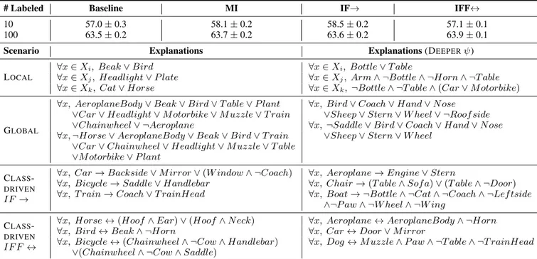
# Labeled Baseline MI IF→ IFF↔
10 57.0 ± 0.3 58.1 ± 0.2 58.5 ± 0.2 57.1 ± 0.1
100 63.5 ± 0.2 63.7 ± 0.2 63.6 ± 0.2 63.9 ± 0.1
Scenario Explanations Explanations (DEEPERψ)
LOCAL
∀x ∈ Xi, Beak ∨ Bird ∀x ∈ Xi, Bottle ∨ T able
∀x ∈ Xj, Headlight ∨ P late ∀x ∈ Xj, Arm ∧ ¬Bottle ∧ ¬Horn ∧ ¬T able ∀x ∈ Xk, Cat ∨ Horse ∀x ∈ Xk, ¬Bottle ∧ ¬T able ∧ (Car ∨ M otorbike)
GLOBAL
∀x, AeroplaneBody ∨ Beak ∨ Bird ∨ T able ∨ P lant ∨Car ∨ Headlight ∨ M otorbike ∨ M uzzle ∨ T rain ∨Chainwheel ∨ ¬Aeroplane
∀x, Bird ∨ Coach ∨ Hand ∨ N ose ∨Sheep ∨ Stern ∨ W heel ∨ ¬Roof side ∀x, ¬Saddle ∨ Bird ∨ Coach ∨ Hand ∨ N ose ∀x, ¬Horse ∨ AeroplaneBody ∨ Beak ∨ Bird ∨ T rain
∨Car ∨ Chainwheel ∨ Headlight ∨ M uzzle ∨ T able ∨M otorbike ∨ P lant
∨Sheep ∨ Stern ∨ W heel
CLASS
-DRIVEN
IF →
∀x, Car → Backside ∨ M irror ∨ (W indow ∧ ¬Coach) ∀x, Aeroplane → Engine ∨ Stern
∀x, Bicycle → Saddle ∨ Handlebar ∀x, Chair → (T able ∧ Sof a) ∨ (T able ∧ ¬Door) ∀x, T rain → Coach ∨ T rainHead ∀x, Boat → ¬Bottle ∧ ¬Cat ∧ ¬Coach ∧ ¬Lef tside
∧¬P aw ∧ ¬W heel ∧ ¬W ing CLASS
-DRIVEN
IF F ↔
∀x, Horse ↔ (Hoof ∧ Ear) ∨ (Hoof ∧ N eck) ∀x, Aeroplane ↔ AeroplaneBody ∧ ¬Horn
∀x, Bird ↔ Beak ∧ ¬Horn ∀x, Car ↔ Door ∨ M irror
∀x, Bicycle ↔ (Chainwheel ∧ ¬Cow ∧ Handlebar) ∨(Chainwheel ∧ ¬Cow ∧ Saddle)
∀x, Dog ↔ M uzzle ∧ P aw ∧ ¬T able ∧ ¬T rainHead
Table 1: PASCAL-Part dataset. Top: macro F1 scores % (±standard deviation), different learning settings and number of labeled points per-class. Bottom: explanations yielded in different scenarios (two types of ψ-network). Functions ˆfi’s are indicated with their class-names.
grid search procedure, with values ranging in [10−1, 10−4], selecting the model that returned the best accuracy on a held-out validation set. Results are averaged over 5 different runs. Each neuron is forced to keep only q = 2 input connections in the ψ-network. Deeper ψ-networks are capable of providing more complex explanations, since the compositional structure of the network can relate multiple predicates. We considered two types of ψ-networks, with one or two hidden layers (10 units each), respectively, with the exception of the case of M I in which we considered no-hidden layers or one hidden layer (10 units). This is due to the unsupervised nature of the M I criterion, that, when implemented in deeper networks might capture more complex regularities. When class-driven criteria are exploited, we considered an independent neural network to implement each ψj associated to a driving class.
The input space of each of them is different, due to the mask-ing of the drivmask-ing task function, as described in Section 3.1. When considering the M I criterion only, we used a single ψ-network with a number of output units m (one for each ψj)
ranging from 10 to 50 (cross-validated).
PASCAL-Part. This dataset is composed of 10,103 labeled images of objects (Man, Dog, Car, Train, etc.) and object-parts (Head, Paw, Beak, etc.). We divided them into three splits, composed of 9,092 training images, 505 validation im-ages, 506 test imim-ages, respectively (keeping the original class distribution). Following the approach of [Donadello et al., 2017], very specific parts were merged into unique labels, leading to c = 64 classes, out of which 16 are main ob-jects that contain object-parts from the other classes. From each image, we extracted 2048 features using a ResNet50 backbone network pretrained on ImageNet. We used 100 hidden units and c output units to implement the f -network. We tested two different semi-supervised settings in which 10
Figure 3: F1 score % on (a) the driving classes and (b) on the other classes, in function of the number of labeled examples per class.
and 100 labeled examples per-class are respectively provided. The remaining portion of the training data is left unlabeled (it is exploited by the learning criteria of Section 3.1). In the class-driven cases, we considered the main objects as driving classes, so m = 16. Results are reported in Table 1, in which the F1 scores (upper portion) and a sample of the extracted rules (lower portion) are shown. The proposed learning crite-ria lead to an improvement of the classifier performance that is more evident when less supervisions are provided, as ex-pected. We further explored this result, distinguishing be-tween the F1 measured (a) on the driving classes, that are more represented, and (b) on the other classes. Fig. 3 (top) shows that evident improvements (w.r.t. the baseline) can sometimes be due to only one of the two groups of classes, and there is not a clear trend among the criteria. Notice that s
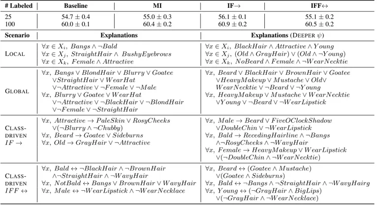
# Labeled Baseline MI IF→ IFF↔
25 54.7 ± 0.4 55.0 ± 0.3 56.1 ± 0.1 55.1 ± 0.2
100 60.0 ± 0.1 60.4 ± 0.2 60.9 ± 0.2 60.5 ± 0.2
Scenario Explanations Explanations (DEEPERψ)
LOCAL
∀x ∈ Xi, Bangs ∧ ¬Bald ∀x ∈ Xi, BlackHair ∧ Attractive ∧ Y oung ∀x ∈ Xj, StraightHair ∧ BushyEyebrows ∀x ∈ Xj, (Old ∧ GrayHair) ∨ (Old ∧ ¬Y oung) ∀x ∈ Xk, F emale ∧ Attractive ∀x ∈ Xk, N oBeard ∧ F emale ∧ ¬W earN ecktie
GLOBAL
∀x, Bangs ∨ BlondHair ∨ Blurry ∨ Goatee ∨StraightHair ∨ W earHat
∨¬Attractive ∨ ¬F emale ∨ ¬M ale
∀x, Beard ∨ BlackHair ∨ BrownHair ∨ Goatee ∨HeavyM akeup ∨ M ustache ∨ Old∨ W earN ecktie ∨ ¬Beard ∨ ¬Y oung ∀x, Blurry ∨ Goatee ∨ W earHat
∨¬Attractive ∨ ¬BlackHair ∨ ¬BlondHair ∨¬F emale ∨ ¬StraightHair
∀x, HeavyM akeup ∨ M ustache ∨ W earN ecktie ∨Y oung ∨ ¬Beard ∨ ¬W earLipstick
CLASS
-DRIVEN
IF →
∀x, Attractive → P aleSkin ∨ RosyCheeks ∨(¬Blurry ∧ ¬Chubby)
∀x, M ale → Beard ∨ F iveOClockShadow ∨DoubleChin ∨ ¬W earLipstick ∀x, Beard → Goatee ∨ Sideburns
∀x, Old → GrayHair ∨ ¬Attractive
∀x, Bald → RecedingHairline ∧ ¬Bangs ∧¬RosyCheeks ∧ ¬W avyHair
∀x, F emale → HeavyM akeup ∨ W earLipstick ∨(¬DoubleChin ∧ ¬W earN ecktie)
CLASS
-DRIVEN
IF F ↔
∀x, Bald ↔ ¬BlackHair ∧ ¬BrownHair ∧¬StraightHair ∧ ¬W avyHair
∀x, Beard ↔ (Goatee ∧ M ustache) ∨(Goatee ∧ Sideburns)
∀x, N otBald ↔ Bangs ∨ BrownHair ∨ W avyHair ∀x, Bald ↔ ¬Bangs ∧ ¬StraightHair ∧ ¬W avyHairg ∀x, M ale ↔ ¬W earLipstick ∧ ¬W earN ecklace ∀x, Y oung ↔ (¬GrayHair ∧ BigLips)
∨(¬GrayHair ∧ ¬W earN ecklace)
Table 2: CelebA dataset. Top: macro F1 scores % (±standard deviation), different learning settings and number of labeled points per-class. Bottom: explanations yielded in different scenarios (two types of ψ-network). Functions ˆfi’s are indicated with their class-names.
class-driven criterion not necessarily leads to better driving-task-functions, while it can also improve the other functions. This is because some driving classes might also participate in explaining other driving classes. The explanations in Table 1 show that deeper ψ networks usually lead to more complex formulas, as expected. Local Explanations depend on the re-gions covered by the Xj, and they sometimes involve
seman-tically related classes, that might be simultaneously active on the same region. Global Explanations show possible cover-ings of the whole classifier output space. We only show 2 sample ˆψ0j’s from Eq. 4. They might be harder to follow, since they merge multiple local explanations. In the deeper case we get more compact terms, that, however, are more nu-merous, i.e., larger K. Class-driven Explanations IF→ and IFF↔ provide a semantically coherent description of objects and their parts. Interestingly, these rules usually implement reasonable expectations on this task, with a few exceptions. The IFF↔ case is more restrictive than IF→ (compare Car, Bicyclein the two cases).
CelebA. This dataset is composed of over 200k images of celebrity faces, out of which 45% are used as training data, 5% as validation data and ≈ 100k are used for testing. The dataset is composed of 40 annotated attributes (classes) per image (BlondHair, Sideburns, GrayHair, WavyHair, etc.), that we extended by adding the attributes NotAttractive, NotBald, Female, Beard, Old, as opposite of the already existing At-tractive, Bald, Male, NoBeard, Young. In the class-driven criteria, these two sets of attributes are the ones we require to explain (c = 10). We exploit the same pre-processing and neural architectures of the previous experiment, evaluating
semi-supervised settings with 25 and 100 labeled examples per class. Results are reported in Table 2 and Fig. 3 (bot-tom). We obtained a slightly less evident improvement of the performance with respect to the baseline, especially in the less-supervised case. This is mostly due to the fact that some classes are associated to high-level attributes (such as Attrac-tive) that might be not easy to generalize from a few supervi-sions. When distinguishing among the results on driving and not-driving classes (Fig. 3), improvements are more evident. From the Local Explanations in the lower portion of Table 2, we can appreciate that some rules are able to capture in a fully unsupervised way the relationships between, for example, be-ing Attractive and Young, or bebe-ing Old and with GrayHair. Global Explanationsshow more differentiated coverings of the classifier output space. Class-driven Explanations IF→ and IFF↔ yield descriptions that, again, are usually in line with common expectations (see Beard, Bald, Male).
5
Conclusions
We presented an approach that yields First-Order Logic-based explanations of a multi-label neural classifier, using an-other neural network that learns to explain the classifier itself. We plan to follow this innovative research direction consider-ing new use-cases and rule types.
Acknowledgements
This work was partly supported by the PRIN 2017 project RexLearn, funded by the Italian Ministry of Education, Uni-versity and Research (grant no. 2017TWNMH2).
References
[Betti et al., 2019] Alessandro Betti, Marco Gori, and Ste-fano Melacci. Cognitive action laws: The case of visual features. IEEE transactions on neural networks and learn-ing systems, 2019.
[Bibal and Fr´enay, 2016] Adrien Bibal and Benoˆıt Fr´enay. Interpretability of machine learning models and represen-tations: an introduction. In ESANN, 2016.
[Carvalho et al., 2019] Diogo V Carvalho, Eduardo M Pereira, and Jaime S Cardoso. Machine learning inter-pretability: A survey on methods and metrics. Electronics, 8(8):832, 2019.
[Donadello et al., 2017] Ivan Donadello, Luciano Serafini, and Artur d’Avila Garcez. Logic tensor networks for semantic image interpretation. arXiv preprint arXiv:1705.08968, 2017.
[Doshi-Velez and Kim, 2017] Finale Doshi-Velez and Been Kim. Towards a rigorous science of interpretable machine learning. arXiv preprint arXiv:1702.08608, 2017.
[Doˇsilovi´c et al., 2018] Filip Karlo Doˇsilovi´c, Mario Brˇci´c, and Nikica Hlupi´c. Explainable artificial intelligence: A survey. In 2018 41st International convention on informa-tion and communicainforma-tion technology, electronics and mi-croelectronics (MIPRO), pages 0210–0215. IEEE, 2018. [Freitas, 2014] Alex A Freitas. Comprehensible
classifica-tion models: a posiclassifica-tion paper. ACM SIGKDD exploraclassifica-tions newsletter, 15(1):1–10, 2014.
[Fu, 1991] LiMin Fu. Rule learning by searching on adapted nets. In AAAI, volume 91, pages 590–595, 1991.
[Guidotti et al., 2018] Riccardo Guidotti, Anna Monreale, Salvatore Ruggieri, Franco Turini, Fosca Giannotti, and Dino Pedreschi. A survey of methods for explaining black box models. ACM computing surveys (CSUR), 51(5):93, 2018.
[Gunning, 2017] David Gunning. Explainable artificial in-telligence (xai). Defense Advanced Research Projects Agency (DARPA), nd Web, 2, 2017.
[Huysmans et al., 2011] Johan Huysmans, Karel Dejaeger, Christophe Mues, Jan Vanthienen, and Bart Baesens. An empirical evaluation of the comprehensibility of decision table, tree and rule based predictive models. Decision Sup-port Systems, 51(1):141–154, 2011.
[Liu, 2007] Bing Liu. Web data mining: exploring hyper-links, contents, and usage data. Springer Science & Busi-ness Media, 2007.
[Melacci and Belkin, 2011] Stefano Melacci and Mikhail Belkin. Laplacian support vector machines trained in the primal. Journal of Machine Learning Research, 12(Mar):1149–1184, 2011.
[Melacci and Gori, 2012] Stefano Melacci and Marco Gori. Unsupervised learning by minimal entropy encoding. IEEE transactions on neural networks and learning sys-tems, 23(12):1849–1861, 2012.
[Melacci et al., 2009] Stefano Melacci, Marco Maggini, and Marco Gori. Semi–supervised learning with constraints for multi–view object recognition. In International Con-ference on Artificial Neural Networks, pages 653–662. Springer, 2009.
[Molnar, 2019] Christoph Molnar. Interpretable machine learning. Lulu. com, 2019.
[Russell and Norvig, 2016] Stuart J Russell and Peter Norvig. Artificial intelligence: a modern approach. Malaysia; Pearson Education Limited,, 2016.
[Sato and Tsukimoto, 2001] Makoto Sato and Hiroshi Tsukimoto. Rule extraction from neural networks via decision tree induction. In IJCNN’01. International Joint Conference on Neural Networks. Proceedings (Cat. No. 01CH37222), volume 3, pages 1870–1875. IEEE, 2001. [Teso and Kersting, 2019] Stefano Teso and Kristian
Kerst-ing. Explanatory interactive machine learnKerst-ing. In Pro-ceedings of the 2019 AAAI/ACM Conference on AI, Ethics, and Society, pages 239–245, 2019.
[Towell and Shavlik, 1993] Geoffrey G Towell and Jude W Shavlik. Extracting refined rules from knowledge-based neural networks. Machine learning, 13(1):71–101, 1993. [Tsukimoto, 2000] Hiroshi Tsukimoto. Extracting rules
from trained neural networks. IEEE Transactions on Neu-ral networks, 11(2):377–389, 2000.
[Witten and Frank, 2005] Ian H Witten and Eibe Frank. Data mining: Practical machine learning tools and techniques 2nd edition. Morgan Kaufmann, San Francisco, 2005. [Zilke et al., 2016] Jan Ruben Zilke, Eneldo Loza Menc´ıa,
and Frederik Janssen. Deepred–rule extraction from deep neural networks. In International Conference on Discov-ery Science, pages 457–473. Springer, 2016.