Integration of the FEMLCORE code in the
SALOME platform
D. Cerroni, R. Da Vià, A. Cervone,
S. Manservisi, F. Menghini and G. Pozzetti
Contents
Introduction 6
1 Code integration in SALOME platform 9
1.1 SALOME C++ library integration . . . 9
1.1.1 Generation of the C++ code library . . . 9
1.1.2 Generation of the a SALOME module by using YACS-GEN . . . . 11
1.1.3 Running a SALOME module by using YACS . . . 13
1.1.4 Running directly with a main program . . . 16
1.2 libMesh-SALOME integration . . . 18
1.2.1 Generation of the code-library . . . 18
1.2.2 libMesh-SALOME interface . . . 19
1.2.3 Implementation of the SALOME-libMesh interface . . . 26
1.3 FEMLCORE-SALOME integration . . . 29
1.3.1 SALOME-FEMLCORE interface . . . 29
1.3.2 Implementation of the SALOME-FEMLCORE interface . . . 36
1.4 Deployment of the SALOME platform on the CRESCO cluster . . . 39
2 FEMLCORE coupling on SALOME 42 2.1 Coupling libMesh modules on SALOME . . . 42
2.1.1 LibMesh energy problem coupling (3D-3D) . . . 42
2.1.2 LibMesh Navier-Stokes coupling (3D-3D) . . . 48
2.1.3 LibMesh energy coupling 3D-module/1D-module . . . 54
2.2 Coupling FEMLCORE modules . . . 57
2.2.1 FEMus Navier-Stokes 3D-CFD module coupling . . . 57
2.2.2 FEMus-libMesh coupling (3D-1D) . . . 63
2.3 Coupling FEM-LCORE on SALOME platform . . . 67
2.3.1 Introduction . . . 67
2.3.2 Exact solution and benchmark cases . . . 69
2.3.3 Benchmarks on FEM-LCORE integration. . . 71 2.3.4 Coupling 3D-FEMLCORE and 1D libMesh primary loop module . 80
Conclusions 88
Bibliography 89
Introduction
Computational simulation of nuclear reactor is of great importance for design, safety and optimal use of fuel resources. Unfortunately a complete simulation of nuclear systems in three-dimensional geometries is not possible with the current available computational power and therefore it is necessary a multiscale approach where the global system is solved at a mono-dimensional level and only some components of interest are solved in great details.
In the previous reports the multiscale code FEMLCORE has been developed for LF reactor of generation IV in the framework of this multiscale approach. Mono-dimensional and three-dimensional modules have been created with appropriate interfaces [2, 3]. Porous modules have been developed for the reactor core where a detailed computation of all the reactor channels inside all the assemblies is not still possible [2, 3, 4]. Simplified freezing modules have been adapted to compute the thermal hydraulics of the reactor when solidification may occur [10, 5].
The mono-dimensional system code implemented in the FEMLCORE module is based on the balance equations [4, 5]. System codes cannot reproduce a multidimensional phys-ical systems such as a nuclear reactor because they are based only on mono-dimensional physical principles and they need experimental data to add the missing information. One of the main goal of the FEMLCORE project is to include, as mono-dimensional modules, system codes validated with nuclear data. In order to do this we must inte-grate the FEMLCORE in the SALOME platform where several nuclear system codes are available.
SALOME is an open source generic platform for preprocessing and postprocessing of numerical simulations, developed by CEA and other institutions [32]. In the plat-form there are modules needed for multi-dimensional CFD computations and for system codes. There are tools for preprocessing CAD applications (GEOM) and for generating meshes (MESH). With the GEOM application one can create, modify, import, export (IGES, STEP and BREP format), repair and fix CAD models. With the MESH appli-cation one can edit, check, import and export meshes (in MED, UNV, DAT and STL formats). These modules are fully integrated in the SALOME platform. There are also postprocessing tools to analyze simulation data such as PARAVIS (PARAVIEW). PAR-AVIEW is an open-source, multi-platform data analysis and visualization application. The data analysis can be done interactively in three-dimension or using PARAVIEW’s batch processing capabilities [28].
This platform has been conceived not only to collect a series of codes that have been extensively used in the field of thermal hydraulics of nuclear reactors but also to harmo-nize them with the aim of solving complex problems by exchanging information among different codes over a common platform and on large multiprocessor architectures.
SA-LOME can also be used as a platform for the integration of external third-party numer-ical codes to produce a new application with full pre and postprocessing management of CAD models.
The European NURESAFE (ex NURISP) project is planned to be based on the SALOME platform. The project has started with the CATHARE, NEPTUNE and TRIO_U codes as independent codes, with not compatible input and output formats [6, 7]. CATHARE is a Code for the Analysis of Thermal Hydraulics during an Acci-dent of Reactor and safety Evaluation for LWR [22]. This system code is used mainly for PWR safety analysis, accident management and definition of plant operating procedures. It is also used to quantify conservative analysis margins and for nuclear reactor licensing [23, 24]. TRIO_U and NEPTUNE codes solve the flow equations in multidimensional geometries with particular attention to two-phase flow [26, 25]. CATHARE, NEPTUNE and TRIO_U are developed by CEA and EDF and they can be used only under NURE-SAFE project agreement. In particular we are interested in the CATHARE system code [22, 23, 24]. The CATHARE system code, like other important nuclear codes, have been developed with an interface on SALOME platform for coupling and integration [24, 27]. At the moment the platform is based on computational tools for light water reactors but many of the codes may be adapted to liquid metals simulations.
The integration of a code on the SALOME platform is obtained by generating an interface with functions available in the MEDMem library (provided in the SALOME platform) that allows the data transfer from the platform to the code and viceversa. Two different codes both with SALOME MEDMem interface can transfer data to the interface and then from the interface to the other code. All the data operations of the SALOME platform involve files in MED (Modèle d’Échange de Données) format. MED is a data storage format based upon the HDF library [35]. The HDF format is largely used and will probably become the standard in a short future. However the implementation in MED format is rare. In the SALOME platform a MED module is implemented. The MED module provides a library for storing and recovering computer data in MED format associating numerical meshes and fields, thus allowing the exchange between different codes and solvers. Inside SALOME these structures are exchanged between solvers at the communication level (CORBA or MPI) offering common read/write functions through MED files.
The MED data model defines the data structures exchanged by codes. The modeled data concern geometrical data and the resulting fields that can be defined on nodes. MED supports eight element shapes: point, line, triangle, quadrangle, tetrahedron, pyramid, hexahedron, polygon and polyhedron. Each element has a different number of nodes, depending on linear or quadratic interpolation. MED defines also numbering conventions and therefore a standard for data storage in HDF5 format. The MED libraries are divided into three groups of functions: MED File, MED Memory and MED CORBA. The first group (MED File) is a C and FORTRAN API that implements mesh and read/write functions into files with .med extension. These files are in HDF5 format. The MED Memory group, which is a C++ and Python API, creates mesh and field objects in memory. Mesh creation can be done using set functions, or by loading a file. Fields are also created loading files or by initialization with user-defined functions.
Finally the group of functions called MED CORBA allows distributed computation inside SALOME [32]. In order to have a working platform, common input and output formats should be harmonized between different codes. This can be achieved by using SALOME as the basic platform taking care of the data exchange between codes and of the distributed computation between different clusters.
In this report we describe the integration of the FEMLCORE code in the SALOME platform. This is the first step in the direction of coupling FEMLCORE with a system code, like CATHARE, to simulate the entire primary loop inside the SALOME platform. The CATHARE-SALOME interface is developed by CEA and EDF and it can be used only under agreement. Therefore in this report we developed a mono dimensional code with the libMesh library. The interface libMesh-SALOME was developed by CEA and EDF for Laplacian and Linear Elasticity solution but libMesh library is open-source software.
Chapter 1 is devoted to the integration of the libMesh and FEMLCORE (FEMus) libraries in SALOME platform. An interface class called FEMUS is developed following the construction of the interface class LIBMESH (developed originally by CEA and EDF) that allows the data transfer from/to FEMLCORE and any platform integrated code.
In Chapter 2 there is a description of many coupling tests carried on with LIBMESH and FEMUS interface. 3D-CFD/3D-CFD coupling for energy and Navier Stokes equa-tions are presented with codes based both on libMesh and FEMus libraries. 3D-CFD/1D-CFD coupling for energy equation are also investigated. Simulations with FEMLCORE (3D-porous) and the FEMUS interface are presented where the interface is used to transfer data for heat generation and pressure drop analytical distributions. Finally a 3D-porous/1D-porous coupling FEMLCORE-libMesh is presented with the simulation of the core of the design reactor ELSY [13, 14, 15, 16, 17, 18]. The core of this reac-tor has been modeled and simulated with a 3D-porous model already implemented in FEMLCORE code, while the external primary loop has been simulated with a simple 1D-porous model implemented with libMesh library.
1 Code integration in SALOME platform
1.1 SALOME C++ library integration
In this section we describe the SALOME platform integration procedure with a generic code. Any code that can be reduced in the form of C or C++ libraries could be therefore integrated in the SALOME platform. The integration procedure ends with the gener-ation of a code module that can run in the SALOME platform with or without GUI support and with or without graphical YACS support for code integration. This allows the user to couple the code at the desired level inside the platform.
We divide the procedure in three steps: generation of the code library,
gener-ation of the SALOME module and finally the implementgener-ation of the module
inside the SALOME platform. The description procedure is based on the FEM-LCORE (FEMus) software, where the FEM-LCORE code is an application of the FEMus code. We assume that FEMus is installed in the directory
pathtoproj/femus
and its FEM-LCORE application in pathtoproj/femus/USER_APPL/femlcore. We use the directory pathtoproj as a main directory where all the software is supposed to be installed (SALOME, FEM-LCORE (FEMus), HDF5, MPI etc..). We assume that SALOME is installed in the directory
pathtoproj/salome
together with the MED libraries in pathtoproj/salome/MED. In order to use the SA-LOME platform the environment should be created by setting
cd pathtoproj/salome source env_products.sh
where the env_products.sh script is available from the package itself in the binary release [32].
The compilation of the SALOME platform is needed to use MPI inside the platform. We remark that if the SALOME is not compiled with MPI then it cannot use MPI to pass MPI parallel information but the code can still run parallel and use MPI on its own [29, 30].
1.1.1 Generation of the C++ code library
In this section we generate a simple code by scratch in order to clarify the SALOME integration procedure. This integration procedure allows the user also to couple any code of the platform with a new one written by the user himself.
As a very simplified example we can consider the integration in the SALOME platform of this simple program: given x and y, the program computes f = x + 3 ∗ y + sin(x). In order to do this we can construct a set of function that can perform addition, multipli-cation, the operation sin and then a main program that combines them to obtain the desired results. The generation of a library code from a set of functions is simple and can be summarized in the following steps. We consider to write a set of functions that we call MATH. We set the application in the directory
pathtoproj/femus/contrib/Myapplication
where the pathtoproj is the directory where all the codes are installed. The application
MATH must consist of the main directory MATHCPP and the sub-directories: src, in-clude, lib. In the sub-directory src we have files *.cxx; in include directory we have files
*.hxx; in lib we have dynamic libraries *.so
Inside the directory include one must write the header files for the C++ object oriented class. For example in order to build the MATH class (no MPI) we construct a class header MATH.hxx defined as #ifndef _MATH_hxx #define _MATH_hxx #include <vector> class MATH { // Simple class public:
double sum(const std::vector<double>& tab); double squareroot(double x);
double plus(double x, double y); double minus(double x, double y); double times(double x, double y); double sinx(double x);
private:
static const double epsilon; static const double pi; };
Inside the directory src one writes the source files. For example the MATH class can be defined by two constants
const double MATH::pi=3.1415926535897931; const double MATH::epsilon=1.0E-12; the default constructor and some functions
double MATH::plus (double x, double y){return x+y;} double MATH::minus(double x, double y){return x-y;} double MATH::times(double x, double y){return x*y;}
double MATH::sinx(double x) {return sin(x);}
The command to generate the dynamic library libMATHCPP.so in the src directory, if the program is parallel, is
mpicxx -o libMATHCPP.so *.cxx -I/pathtoproj/femus/contrib/ Myapplication/MATHCPP/include/ -lmpi -shared -fPIC or
g++ -o libMATHCPP.so *.cxx -I/pathtoproj/femus/contrib/
Myapplication/MATHCPP/include/ -lmpi -shared -fPIC
in the serial case. A file appears with name libMATHCPP.so which is the dynamic library just created. We move libMATHCPP.so in the lib directory with the name libMATHCXX.so.
Finally we should have in src the file MATH.cxx, in include the header MATH.hxx and in lib the dynamic library libMATHCXX.so. By starting from a set of functions we have now a library of functions.
1.1.2 Generation of the a SALOME module by using YACS-GEN
At this point we have the directory Myapplication which has MATH.cxx in src , MATH.hxx in include and libMATHCXX.so in lib. The environment for MATHCPP can be set by export MATHCPP_ROOT_DIR=/pathtoproj/femus/
contrib/Myapplication/MATHCPP/
In order to create a SALOME module with relative YACS functions one must run a python script by typing
python math_component.py
The script will use YACS-GEN module to generate the needed functions and modules and it can be written only in python language. This is the general form for the script: #! /usr/bin/env python
import os
from module_generator import Generator,Module,Service,HXX2SALOMEComponent # Generator python function generates the code
#
# grab from environment variables of interest (set by source env_products) kernel_root_dir=os.environ["KERNEL_ROOT_DIR"]
gui_root_dir=os.environ["GUI_ROOT_DIR"] yacs_root_dir=os.environ["YACS_ROOT_DIR"]
salome_env="pathtoproj/salome/env_products.sh" #
# create a context, that provide environment information context={’update’:1, "makeflags":"-j2", "prerequisites":salome_env, "kernel":kernel_root_dir, "gui":gui_root_dir, "yacs":yacs_root_dir } #
# specify a SALOME modules called MATHEMATICS, including one SALOME # component called MATH
module="MATHEMATICS" components_name=["MATH"] components=[]
for compo_name in components_name:
cpp_root_dir="pathtoproj/femus/contrib/Myapplication/MATHCPP" # print
print compo_name, components_name, cpp_root_dir
# generation of class components
components.append(HXX2SALOMEComponent("MATH.hxx",
"libMATHCXX.so",cpp_root_dir ) ) # we ask to install the module in pathtoproj/salome/MATHEMATICS module_root_dir="pathtoproj/salome/MATHEMATICS"
# generate and compile the salome component with yacsgen
g=Generator(Module(module,components=components,prefix=module_root_dir), context) g.generate() g.bootstrap() g.configure() g.make() g.install() #
# generate a SALOME application containing :
# - the MATHEMATICS module,
# - the native modules GUI, YACS
g.make_appli("appli_math", restrict=["KERNEL"],
altmodules={"GUI":yacs_root_dir, "YACS":yacs_root_dir})
The generated module is labeled MATH and it is installed in the SALOME module directory in a new directory called MATHEMATICS. Note that if SALOME is compiled with MPI (this is not the default) then the function HXX2SALOMEParaComponent should be used in the above script, replacing HXX2SALOMEComponent.
1.1.3 Running a SALOME module by using YACS
After running the script in the main directory Myapplication we have two new sub-directories, MATHEMATICS_SRC and appli_math and two files, parse_result and
parse_type_result. The directory MATHEMATICS_SRC is the build directory. The appli_math is the directory where the application MATHEMATICS can be launched. A
new directory named MATHEMATICS appears in the SALOME main directory
pathto-proj/SALOME. This module consists of an include, src, idl and lib sub-directories.
The file parse_result contains the parsing of the function prototypes. In our case the
file parse_result is Function;double;sum const std::vector<double>&;tab Function;double;squareroot double;x Function;double;plus double;x double;y Function;double;minus double;x double;y Function;double;times double;x double;y Function;double;sinx double;x
This script generates the new directory idl in the module MATHEMATICS. Each func-tion prototype is translated in a different language by parsing the return type and the type argument. For example the prototype double sum(double x,double y) gives double as a function return type and has two double input variables. These functions are used for YACS graphical representation. Before running the code one must set the environment for the module with
export MATHEMATICS_ROOT_DIR=pathtoproj/salome/MATHEMATICS/
From the directory appli_math one can start SALOME with this MATH module. Inside this directory two files are important: config_appli.xml and SalomeAppli.xml.
The file config_appli.xml contains <application>
<prerequisites path="pathtoproj/salome/env_products.sh"/> <modules>
<module name="KERNEL" path="pathtoproj/salome/KERNEL_7.3.0"/> <module name="YACS" path="pathtoproj/salome/YACS_7.3.0"/> <module name="GUI" path="pathtoproj/salome/YACS_7.3.0"/>
<module name="MATHEMATICS" path="pathtoproj/salome/MATHEMATICS"/> </modules>
</application>
where one can see the modules loaded when starting the platform. By adding the location of the GEOM, SMESH, PARAVIS modules the platform can consider the loading of the GEOM, SMESH and PARAVIS modules too [28]. The file SalomeAppli.xml contains <document>
<section name="launch">
<!-- SALOME launching parameters -->
<parameter name="gui" value="yes"/>
<parameter name="splash" value="yes"/>
<parameter name="file" value="no"/>
<parameter name="key" value="no"/>
<parameter name="interp" value="no"/>
<parameter name="logger" value="no"/>
<parameter name="xterm" value="no"/>
<parameter name="portkill" value="no"/>
<parameter name="killall" value="no"/>
<parameter name="noexcepthandler" value="no"/>
<parameter name="modules" value="YACS,MATHEMATICS"/>
<parameter name="pyModules" value=""/>
<parameter name="embedded" value="SalomeAppEngine,study,
cppContainer,registry,moduleCatalog"/> <parameter name="standalone" value=""/>
</section> </document>
By substituting YACS, MATHEMATICS with YACS, MATHEMATICS, GEOM, SMESH, PARAVIS the platform starts with GEOM, SMESH and PARAVIS modules too. Before starting SALOME the MATHCPP and MATHEMATICS libraries should be included in the LD_LIBRARY_PATH by typing
export LD_LIBRARY_PATH=pathtoproj/femus/contrib/
Myapplication/MATHCPP/lib/:$LD_LIBRARY_PATH export LD_LIBRARY_PATH=pathtoproj/salome/MATHEMATICS/lib/
Figure 1.1: YACS with MATH module integration
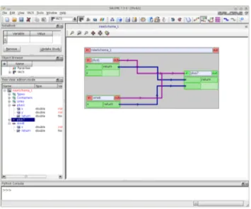
Figure 1.2: Building YACS schema for f(x, y) = x + y + sin(x). Now we start the YACS module by typing
cd appli_math ./runAppli
If only the YACS and MATHEMATICS modules are in the platform then SALOME starts with no active modules. One must select the new option from the menu to use the YACS module. If more than one module is loaded then a menu appears. We select YACS module and then Create a new YACS schema. From Figure 1.1 one can note
Figure 1.3: Running YACS schema for f(x, y) = x + y + sin(x).
that the functions minus, plus, sum and sin(x) from the MATH module appear on the catalog panel. In order to construct the graphical YACS program that computes
f(x, y) = x + y + sin(x) we drag a sum, a sin and a sum function again from the catalog
to the main schema. We connect the return of the plus1 schema block to the x of the
plus7 block and the return of the sin8 block to the y of the plus7 block. After this we
have a situation as depicted in Figure 1.2.
From the input panel we set the initial x and y value. Then from the menu at the top we choose Prepare the schema for run (gear button). A new schema appears which is not editable, from here the code can be run. The tree view on the left shows computation values and errors. It is important to note that an MPI code runs in the YACS schema only if SALOME is compiled with MPI. This may be a limitation in the use of the YACS module since not all MPI functions are implemented correctly in SALOME. However the program can be run in parallel without the use of the graphical environment YACS as it is explained in the next section.
1.1.4 Running directly with a main program
The same program can be run by using a simple main program. For example the same result of the YACS module can be obtained with the following simple program
#include "MATH.hxx" #include <stdio.h> #include <cmath> int main(){ MATH a; double x=1.;
double y=2.; double t=a.plus(x,y); double s=a.plus(t,sin(x)); printf(" %f", s); return 0; }
This implies that in the SALOME platform a code can run both graphically (YACS) or through simple C or C++ programs. In order to compile this program we must include all the libraries and the paths to MATHCPP directory and MATHEMATICS module. Then the executable program can be launched directly by the YACS graphical interface with a Pyscript which can be found in the catalog in the elementary node section of the YACS module.
1.2 libMesh-SALOME integration
The integration of a stand-alone code is more complex but very similar. In this section we describe the integration of the libMesh library in SALOME platform with the aim of using computational modules generated with this library for multiscale coupling. In particular we are interested in coupling 1D modules written with libMesh library with the 3D FEM-LCORE applications using MEDMem library. The libMesh applications are open-source. The integration of an open-source code can be divided into three steps:
generation of the code-library from the code, generation of the MEDMem in-terface and SALOME-libMesh inin-terface integration. The source code is available
and one can see how they are build. In non open-source code like CATHARE the source code is not available but we have the binary version of the library. In this case we can get over the first step of generation of the code-library and go directly to the second step.
1.2.1 Generation of the code-library
The generation of the dynamic library from a code is pretty straightforward for modern codes since they are already built as libraries. The main code is simply a collection of call functions to libraries where the algorithms are developed. For old codes, especially in FORTRAN, sometimes a monolithic main program is developed with a few functions in support with experimental data. In this case is straightforward, for developers, to rebuild the code using a library structure. The libMesh code is built using libraries and therefore, after the code installation, nothing should be done.
LibMesh is a parallel solver for PDE which uses the PETSC libraries as a main package solver. The open MPI is supposed to be installed in
pathtoproj/openmpi-1.4.5/
The version 1.4.5 is installed but the procedure should work also for any upgrade. The installation of the open-mpi libraries is really easy and standard. For details see [30]. The PETSC library is supposed to be installed in
pathtoproj/petsc-3.4.3
The version 3.4.3 is installed but the procedure should work also for others. We use the
opt version and not the dbg version which one could use for debugging. For further
details see [31].
We suppose that the libMesh code is installed in pathtoproj/libmesh-0.9.2.2/
The installation can be easily obtained by following the standard procedure on [34]. The libMesh version is the 0.9-2.2. The integration described here does not work for library below version 0.9. The libMesh main directory must contain the lib and the include sub-directories. In the lib sub-directory the dynamic library libmesh_opt.so.0 is located. The dynamic library libmesh_opt.so.0 contains all the functions in binary form. In the
include sub-directory the prototypes are available for obtaining the documentation and
to compile.
1.2.2 libMesh-SALOME interface
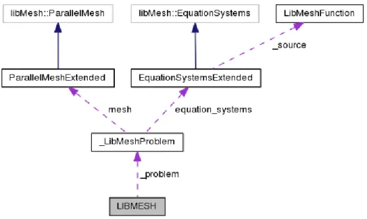
Figure 1.4: Collaboration diagram of the LIBMESH class inside the LibMeshCpp interface
Overview. The interface, called LibMeshCpp, between the MEDMem and the libMesh
libraries consists basically of five classes: LIBMESH, LibMeshProblem, EquationSystem-sExtended, ParallelMeshExtended and LibMeshFunction. All these classes are located in
pathtoproj/femus/contrib/Libmesh_cpp/
Each class has a file and a header with the class name and different extension. The LIBMESH class is the interface with the SALOME platform as it is shown in the collabo-ration diagram in Figure 1.4. This diagram illustrates how the LIBMESH class (interface to SALOME) transfers data to the LibMeshProblem class. In order to interact with the libMesh library two libMesh classes have been extended: the libMesh::EquationSystems and the libMesh::ParalellMesh.
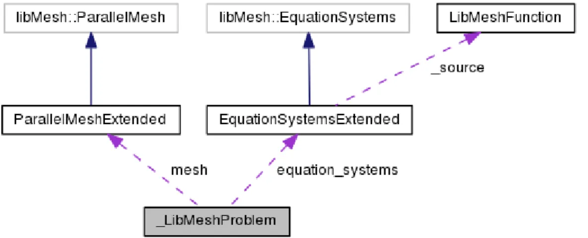
The EquationSystemsExtended class, which uses only MEDMem functions, inherits the libMesh::EquationSystems which uses only libMesh functions as shown in Figure 1.5. The libMesh::EquationSystems contains the assembly and solver of the libMesh code. The data from the LIBMESH class can be transferred into the assembly routine which is user accessible. The data can also be transferred in the opposite direction from the
Figure 1.5: Inheritance diagram of the EquationSystemsExtended class
class is ensured by the C++ inheritance rules. The flow in opposite direction is defined by a dynamic_cast command that allows to use son class functions from the parent class. For this reason the parent class should be polymorphic with at least one virtual function.
Figure 1.6: Inheritance diagram of the ParallelMeshExtended class
Also the mesh class has to be extended. As shown in Figure 1.6 the
ParallelMeshEx-tended class, which uses only MEDMem functions, inherits the original class libMesh::ParallelMesh
which uses only libMesh functions. As in the previous class, data from the LIBMESH class can be transferred, by using a dynamic_cast statement, into the assembly routine which is user accessible. Data can also be transferred in the opposite directions from the libMesh::ParallelMesh to the MEDMem interface through parent to son class inher-itance rules. We recall again that the parent class should be polymorphic with at least one virtual function.
The LIBMESH interface class to SALOME. The LIBMESH class contains the
SA-LOME platform commands. All the code interfaces must have similar commands to run the code from the same main program. Data in the LIBMESH class consist of a simple vector of string of boundary name. The boundary are defined by using the GEOM and the SMESH modules of the SALOME platform.
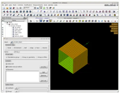
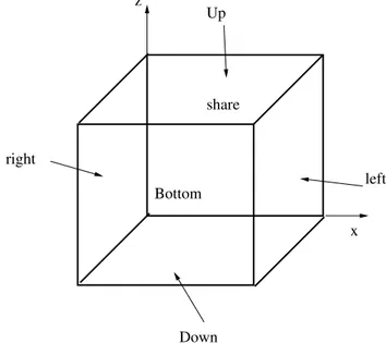
In order to generate a mesh with boundary we open the SALOME platform and the GEOM module as in Figure 1.7. From the menu we open the Create a Box button and select the box dimensions. Then we select Create a Group with option face and
no restriction and click on the desired face. We label six different faces as up, down, left, right, bottom and share. We open the SMESH module and generate the mesh for
the volume and the label for the boundary interfaces, see Figure 1.8. The boundary names and their flags are stored in the LIBMESH interface class. Over these boundaries and volume regions defined by using MEDMem functions we should be able to impose
Figure 1.7: Generation of the boundary with the GEOM module
Figure 1.8: Generation of the boundary name in the SMESH module
values taken by other SALOME platform codes. The functions that start and stop the code are the constructor LIBMESH(MPI_Comm comm) and the function terminate(). These functions take into account the start and stop of all MPI parallel processes of the code. The commands
void setType (const std::string &pbName) void setMesh (const std::string &meshFileName) void solve ()
are used to set the type of the problem (Navies-Stokes, energy, etc.) and the mesh. The mesh should be available in MED and libMesh format for data exchange. The MED format allows data transfer to other codes that use the same format. The solve command controls the solution of the discrete system.
The boundary should be controlled for input and output. For input we have the following interface functions
void setSource (const ParaMEDMem::MEDCouplingFieldDouble *f) void setAnalyticSource (const std::string &f)
void setAverageSources (int n, double val[])
void setAnalyticBoundaryValues (const std::string &name,
const std::string &typeBC, const std::string &f) void setFieldBoundaryValues (const std::string &name,
const std::string &bcType, const ParaMEDMem::MEDCouplingFieldDouble *bcField) For output we have
std::string getBoundaryName (int i)
std::vector< std::string > getBoundaryNames () ParaMEDMem::MEDCouplingFieldDouble * getOutputField
(const std::string &vName) const ParaMEDMem::MEDCouplingFieldDouble * getValuesOnBoundary
(const std::string &name, const std::string &vName) const ParaMEDMem::MEDCouplingFieldDouble * getValuesOnBoundary
(const std::string &name, std::vector< char * > vName) const ParaMEDMem::MEDCouplingFieldDouble * getValuesOnBoundary_nodes
(const std::string &name, std::vector< char * >) const The solution values can be transfer on NODES or CELLS. In this SALOME interface the solution values are collected for CELLS or NODES but set only for CELLS.
LibMeshProblem class as interface class to libMesh code. The interface to libMesh
code is obtained through the LibMeshProblem class. Since the equation system has the mesh pointer of the original code the extended class is not available. For this reason the LibMeshProblem class should access to both ParallelMeshExtended and Equation-SystemsExtended classes as shown in the collaboration diagram of the LibMeshProblem class in Figure 1.9.
The LibMeshProblem class has been specialized for different physics. As one can see in Figure 1.10 this class is inherited by all the physical modules. We have constructed many modules for coupling. We have the energy equation in 1D, 2D and 3D and we call
Figure 1.9: Collaboration diagram of the LibMeshProblem class.
Figure 1.10: Inheritance diagram of the LibMeshProblem class.
it Convection-diffusion problem (Con_DiffProblem). We have the Laplace and Navier-Stokes problem in one, two and three dimensions. For the system scale we have a specific module called Monodim_Problem that can simulate pump, heat exchanger and source term for taking into account the whole loop of interest. Finally we have also a module for structural mechanics computations called LinearElasticity_Problem, available only for 2D computations like plates and sheets. In table 1.1 we have a summary of these modules and their relative scale of interest.
The ParallelMeshExtended class is an extension of the libMesh class ParallelMesh. This extension defines the map between the mesh nodes and elements in MEDMem and libMesh format. In particular the extension class contains the mesh in the ParaMED-MEM::MEDCouplingUMesh class format and all maps
Physics Name module scale
Energy equation Con_DiffProblem 1D,2D,3D
Navier-Stokes equations NS_Problem 2D
NS_Problem3D 3D
System equation Monodim_Problem 1D
Structural mechanics LinearElasticity_Problem 2D
Laplace equation LaplaceProblem 1D,2D,3D
Table 1.1: Multiphysics modules available in LibMesh for coupling.
_node_id: node MEDmem mesh -> node libMesh mesh
_proc_id: processor MEDmem mesh -> processor libMesh mesh
_elem_id: element MEDmem mesh -> element libMesh mesh
that allow the data transfer from one format to another.
The EquationSystemsExtended class is an extension of the libMesh class
EquationSys-tems. The extension contains two standard maps
std::map< int,LibMeshFunction * > _bc
std::map< int, BCType > _bc_type
that associate to any boundary a LibmeshFunction and a BCType. The BCType are the keywords Neumann or Dirichlet depending on the desired boundary condition. A database of these keywords can be updated by the user. The LibmeshFunction is a class object that completes the definition of the boundary conditions. The collaboration diagram of this class is shown in Figure 1.11. In the EquationSystemsExtendedM class
Figure 1.11: Collaboration diagram of the EquationSystemsExtended class new functions are available in addition to the original EquationSystems functions. The following functions are used to set source fields computed by external codes
void setSource (const ParaMEDMEM::MEDCouplingUMesh *mesh, const char *s) void eraseSource ()
void setAverageSources (int n_AverageSources, double Average[]) double getAverageSources (int i)
A coupling volumetric field can be transferred to a LibMesh computation by using
set-Source function. The field is defined over a ParaMEDMEM::MEDCouplingUMesh mesh
which is a MEDMem mesh format. A volumetric field can be extracted from a libMesh solution and transferred to a LibMeshFunction with a MEDMem mesh format by using the getSource function. If the data transfer is between 3D and 1D the average source functions may be used.
The boundary conditions should be transferred from a code to another. Here we can use the following functions to add or erase a boundary coupling
int addBC (const ParaMEDMEM::MEDCouplingUMesh *b) void eraseBC (libMesh::boundary_id_type id) or to set specific field and boundary condition type
void setBCType (libMesh::boundary_id_type id, BCType type) void setBC (libMesh::boundary_id_type id, const char *s) void setBC (libMesh::boundary_id_type id,
const ParaMEDMEM::MEDCouplingFieldDouble *f) void setNodeBC (libMesh::boundary_id_type id,
const ParaMEDMEM::MEDCouplingFieldDouble *f) LibMeshFunction * getBC (libMesh::boundary_id_type id)
BCType getBCType (libMesh::boundary_id_type id)
The boundary labels and types can be imposed by using GEOM and SMESH modules in the SALOME platform, as already described.
The transfer data function. The data are transferred through an object class called
LibmeshFunction. The data in these class are
const libMesh::MeshBase * _mesh
const ParaMEDMEM::MEDCouplingUMesh * _support
ParaMEDMEM::MEDCouplingFieldDouble * _f
std::map< int, int > _nodeID
std::map< std::pair< int, int >, int > _faceID
std::map< int, int > _elemID
The _mesh pointer points to the mesh in libMesh format while _support contains the mesh in MEDMem format. The solution of the internal or external problem in MEDMem format are stored in the field _f. The _f pointer may refer to the part of the mesh
(_support) where the data are to be transferred. In fact if the function is associated
with a part of the boundary, the mesh and its solution is relative only to this part. The
_nodeID, _faceID and _elemID are the maps from the libMesh to the MEDMem mesh
The LibmeshFunction is used to evaluate the field at the boundary and to map the node and element connectivity between coupling codes. Each code has a MEDMem interface which is used to exchange data through the SALOME platform during execution. 1.2.3 Implementation of the SALOME-libMesh interface
In order to explain the code implementation of the data transfer we consider a simple example with the energy equation implemented in the LibMesh module conv-diff. We consider the domain [0, 1]×[−1, 0]×[0, 1] which is the same geometry generated in section 1.2.2. The mesh consists of 12 × 12 × 12 HEX20 quadratic elements. By using GEOM and SMESH modules we have marked the boundary of the domain as up and down in the z direction, left and right in the x direction and bottom and share in the y direction as shown in Figure 1.12. We solve the energy equation that takes into account convection
right left Up Down Bottom share x z
Figure 1.12: Geometry of the test case.
with constant velocity v = (0, 1, 0). The boundary has homogeneous Dirichlet boundary condition on the up, down, left and right faces. On the share face we set homogeneous Neumann boundary conditions while on the bottom we import a constant field from the MEDMem interface. The LibMesh code runs through the LIBMESH class in a few lines:
LIBMESH P;
P.setType("convdiff"); P.setMesh(dataFile); getInput(P, boundary);
for(int i=0; i<boundary.size(); i++) { sBC & b = boundary[i];
if(b.isAnalytic)
P.setAnalyticBoundaryValues(b.name,b.type,b.equation); else P.setFieldBoundaryValues(b.name, b.type, b.field); }
P.solve(); }
The interface P class is constructed in the first statement. The problem type (convdiff) is set with the setType function. The mesh in MED format is assigned with setMesh function which copy the mesh to the LibMesh program in LibMesh format. The interface conditions are set by getInput function which is set by the user.
In order to set the interface conditions the name of the different boundaries should be associated with the boundary conditions. The labels of the boundary regions are available calling the function getBoundaryNames() in the LIBMESH class. A simple statement as
std::vector<std::string> bcNames = P.getBoundaryNames();
returns the name of all the boundary regions. For each region a boundary structure sBC should be defined. This structure is defined as
struct sBC { std::string name; std::string type; bool isAnalytic; std::string equation; MEDCouplingFieldDouble * field; };
The name is the identity label of the boundary region. The type of boundary condition is “Dirichlet” or “ Neumann”. If the isAnalitic is true then an analytic condition is expected if false a numerical field is assigned. The analytical expression is defined in the string equation by using symbolic language. The numerical field is assigned through the pointer field. The solution computed from other codes can be transferred into this field pointer becoming available to the LibMesh code. In our case we build a vector of
sBC structures called boundary and set the appropriate structure in the "Bottom" region
which is the active interface. In this active face we set bcNames[0]=="Bottom";
boundary[0].type = "Dirichlet"; boundary[0].isAnalytic = true; boundary[0].field = NULL; boundary[0].equation = "1.";
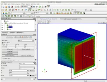
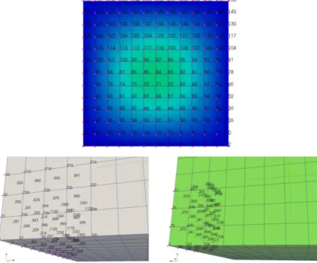
Figure 1.13: Common surface Bottom of the computation domain where the data trans-fer is allowed. Libmesh global numbering.
Figure 1.14: Solution when a surface allows a transfer of data.
Now at each time step the boundary condition defined by the external field field or any analytical expression equation is imposed. In Figure 1.13 one can see the surface (labeled as Bottom) of the computation domain where the data transfer is allowed with Libmesh global numbering. The LIBMESH interface creates a map to connect this global numbering to the surface mesh. The surface mesh in MEDMem representation has the same number of nodes but different numbering. It is necessary therefore to search point by point the correspondence. Once the map is computed all field values on the surface can be passed to the LibMesh surface and viceversa. When the interface condition is transferred then on the Bottom part of the boundary a constant field is applied as one can see from Figure 1.14.
1.3 FEMLCORE-SALOME integration
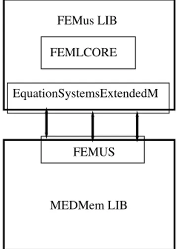
1.3.1 SALOME-FEMLCORE interface FEMUS MEDMem LIB EquationSystemsExtendedM FEMLCORE FEMus LIBFigure 1.15: Diagram of the FEMUS class inside the MEDMem interface
Overview. FEMLCORE is an application of the FEMus library aimed at computation
of 3D core thermal-hydraulics of a fast nuclear reactor. It is therefore interesting to integrate the FEMus library with SALOME platform by writing a MEDMem interface in order to be able to couple the 3D computation of the core obtained by FEMLCORE with a system code simulation, like CATHARE or RELAP. The interface between the MEDMem and the FEMus libraries consists basically of four classes: FEMUS,
Equation-SystemsExtendedM, ParallelMeshExtendedM and LibMeshFunctionM. All these classes
are located in the src and include FEMus directories. As shown in the diagram of Figure 1.15, the FEMUS class is the interface between the library FEMus and the SALOME platform. The FEMUS interface allows to pass commands from MEDMem library to the EquationSystemsExtendedM class which is the problem solver core. This diagram illustrates as the FEMUS class (interface to SALOME) transfers the data to the
Equa-tionSystemsExtendedM class. In order to interact with the FEMus library two FEMus
classes have been extended: the MGEquationsSystem and the MGMesh. The extensions are simply named as EquationsSystemExtendedM and ParalellMeshExtendedM, respec-tively.
The EquationSystemsExtendedM class, which uses only MEDMem functions, inherits the EquationSystems which uses only FEMus functions as shown in Figure 1.16. The
EquationSystems contains the assembly and solver of the FEMus code. The data from
the FEMUS class can be transferred into the assembly routine by a dynamic_cast op-erator. The dynamic_cast operator is a part of the run-time type information (RTTI) system that allows to use son class functions from the parent class. Data can also be transferred in the opposite direction from the EquationSystems to the MEDMem
inter-Figure 1.16: Inheritance diagram of the EquationSystemsExtendedM class
Figure 1.17: Inheritance diagram of the ParallelMeshExtendedM class
face by standard C++ inheritance rules. The MGMesh class contains the multilevel mesh in FEMus format. In order to interface FEMus with MEDMem library a new mesh format should be introduced and the mesh class should be extended. As shown in Figure 1.17 the ParallelMeshExtendedM class, which uses only MEDMem functions, inherits the MGMesh which uses only libMesh functions. In FEMus library, differently from LibMesh library, the mesh is known inside the EquationSystemsExtendedM class and therefore the interface FEMUS class does not need to communicate directly to the
ParallelMeshExtendedM class. As in the class before the data from the FEMUS class
can be transferred by using a dynamic_cast operator into the assembly routine which is user accessible.
The FEMUS interface class to SALOME platform. The FEMUS class is the unique
interface class. It contains data from both FEMus and MEDMem libraries in order to transfer data from one mesh to another (MGMesh to MED). Therefore inside this class there are both pointers _mg_mesh, _med_mesh to their respective MGMesh and MED formats. The FEMUS class needs information to extract data from these different mesh structures. In particular, as shown in 1.18, the classes MGUtils, MGGeomEL,
MGFEMap and MGFemusinit are available inside FEMus to transfer basic information
such as file names, parameters, multigrid level, fem elements etc.. The MGUtils con-tains all the file names and input parameter values. The MGGeomEL and MGFEMap contain information about the finite element mesh structure and MGFemusinit class is the manager class for MPI and multigrid solvers.
Figure 1.18: FEMUS class data to communicate with the FEMus library. one for the mesh and another for the boundary conditions. The mesh structure is called
interface_mesh and consists of
int id;
std::string name;
ParaMEDMEM::MEDCouplingUMesh * support;
where id is the integer number identity and name the name of the common interface. The support is the mesh in MED format. This in general is not the whole mesh but only the mesh for the interested interface region. Since this is a portion of the mesh numbering is different from the global one and a map is needed. There is one interface_mesh structure for each mesh interface of interest. The boundary conditions structure is called UsersBC and consists of
std::string name; std::string type; int from_cmp; int n_cmp; int order_cmp; bool isAnalytic; std::string equation; ParaMEDMEM::MEDCouplingFieldDouble * field; bool on_nodes;
The name is the name of the interface while type refers to the “Mark” or “UnMarked” flag that is used to construct the mesh map. If the interface is “Marked” the code prepares all the tools for the data exchange including an MGMesh-MED map for field exchange. The from_cmp and n_cmp define the first and the number of variables to be exchanged, respectively. The interpolation order is defined by order_cmp. A quadratic variable (on Hex27, Quad9, Tri6 or Tetra10, for example) should have order_cmp=2. If on the surface one desires to impose an analytic function then the Boolean variable
string equation. For numerical fields the MED solution should be transfer through the
field pointer as node or element values by setting the Boolean on_nodes of the UsersBC
structure. There is one UsersBC structure for each mesh interface of interest and all of them are collected in the std::vector< UsersBC > _boundary.
The FEMUS class contains the SALOME platform commands. All the code interfaces must have similar commands to run the code from the same main program. The functions that start and stop the code are the constructor FEMUS(MPI_Comm comm) and the function terminate(). These functions take into account the start and stop of all MPI parallel processes of the code. The initialization of the parameters and the FEM elements are obtained by the following functions
void init_param(MGUtils &mgutils);
void init_fem(MGGeomEl & mggeomel,MGFEMap & mgfemap); The commands
void setSystem(const std::vector<NS_FIELDS> & pbName); void setMesh();
void setMedMesh(const std::string & meshFile);
are used to set the type of the problem (Navies-Stokes, energy, etc.) and the mesh. The
NS_FIELDS enumeration collects the name of some of the implemented modules as
NS_F =0, // [0] -> Navier-Stokes (quadratic (2),NS_EQUATIONS)
NSX_F =0, // [0] -> Navier-Stokes (quadratic (2),NS_EQUATIONS)
NSY_F =1, // [1] -> Navier-Stokes (quadratic (2),NS_EQUATIONS)
NSZ_F =2, // [2] -> Navier-Stokes (quadratic (2),NS_EQUATIONS)
P_F =3, // [3] -> Pressure (linear (1),NS_EQUATIONS==0 or 2)
T_F =4, // [4] -> Temperature (quadratic (2),T_EQUATIONS)
K_F =5, // [5] -> Turbulence K (quadratic (2),TB K_EQUATIONS)
EW_F =6, // [6] -> Turbulence W (quadratic (2),TB W_EQUATIONS)
KTT_F =7, // [7] -> Turbulence K (quadratic (2),TB K_EQUATIONS)
EWTT_F=8, // [8] -> Turbulence W (quadratic (2),TB W_EQUATIONS)
SDSX_F=9, // [9] -> Displacement (quadratic (2), DS_EQUATIONS)
SDSY_F=10, // [10] -> Displacement (quadratic (2), DS_EQUATIONS)
SDSZ_F=11, // [11]-> Displacement (quadratic (2), DS_EQUATIONS)
DA_F =12, // [12]-> DA solver (quadratic (2), DA_EQUATIONS)
DA_P =13, //[13]-> DA solver (piecewise, DA_EQUATIONS)
TA_F =14, // [13]-> Temp adjoint
FS_F =15 // [13]-> Temp adjoint
For example, a vector pbName defined as pbName[0]=NS_F, pbName[1]=T_F defines a problem which consists of the Navier-Stokes and energy equations. The solution of the system is obtained by using these commands
void solve_setup (int &t_in, double &time)
void solve_onestep (const int &t_in, const int &t_step, const int &print_step, double &time, double &dt)
The solve_setup initializes system at t = 0. The solve_onestep function controls a single time step of the problem while solve() can be used to solve more time steps at once.
The boundary should be controlled for input and output. For input we have the following interface functions
setSource (const ParaMEDMEM::MEDCouplingFieldDouble *f) void setAnalyticSource (const std::string &f)
void setAverageSources (int n, double val[])
void setAnalyticBoundaryValues (const std::string &name, int n_cmp, const std::string &typeBC, const std::string &f) void setFieldBoundaryValues (const std::string &name, int n_cmp,
const std::string &bcType,
const ParaMEDMEM::MEDCouplingFieldDouble *bcField) For output we have
std::string getBoundaryName (int i)
std::vector< std::string > getBoundaryNames ()
ParaMEDMEM::MEDCouplingFieldDouble getValuesOnBoundary ( const std::string &nameBC, const std::string &systemName) ParaMEDMEM::MEDCouplingFieldDouble *getValuesOnBoundary(
const std::string &nameBC,
const std::string &systemName, int iCmp) ParaMEDMEM::MEDCouplingFieldDouble * getValuesOnBoundary (
const std::string &nameBC, const std::string &systemName, int Cmp0, int nCmp)
The solution values can be transferred only on nodes.
The interface in this library must be used in different step. They must be initialized, marked and then used. For this reason we have different interface functions
void init_interfaces (const std::string &medfilename, const int index_mgmesh=0, const int index_medmesh=0) void init_interfaces (const std::string &medfilename,
const std::string &medfile_namePold,const FEMUS &P_old, const int index_mgmesh=0, const int index_medmesh=0) void set_param_BCzone ()
void set_param_BCzone (FEMUS &P1)
void init_BCzone (std::vector< std::string > &bcNames) void set_interface_userbc ()
Figure 1.19: Collaboration diagram of the ParallelMeshExtendedM class
The ParallelMeshExtendedM class. The ParallelMeshExtendedM class is an extension
of the FEMus class MGMesh. This extension defines the map between the mesh nodes and elements in MEDMem and libMesh format. In particular the extension class contains the mesh in the ParaMEDMEM::MEDCouplingUMesh class format and all the maps
_node_id: node MEDmem mesh -> node libMesh mesh
_proc_id: processor MEDmem mesh -> processor libMesh mesh
_elem_id: element MEDmem mesh -> element libMesh mesh
that allow the data transfer from one format to another.
Moreover this class contains one standard map and two vector flags std::map< int, int > _bd_group
std::vector< int > _bc_id std::vector< int > _mat_id
The first associates the integer names to an integer. We recall that the names for the boundary and volume zones must be integer number in the range [10, 10000] and [1, 9], respectively. The vector _bc_id contains the boundary flag at each node of the integer name ([10 − 10000]) of the surface/interface . The vector _mat_id contains the boundary flag with the integer name ([1 − 9]) of the volume/material at each node. The collaboration diagram is shown in Figure 1.19.
The EquationSystemsExtendedM class. As shown in Figure 1.20 the
EquationSys-temsExtendedM can access to the mesh classes and to the FEMUSFunction class. In
order to transfer data from MEDMem and FEMus library new functions are available in addition to the original EquationSystems functions.
The following functions are available to set source fields computed by external codes void setSource (const ParaMEDMEM::MEDCouplingUMesh *mesh,
Figure 1.20: Collaboration diagram of the EquationSystemsExtendedM class void eraseSource ()
FEMUSFunction * getSource ()
void setAverageSources (int n_AverageSources, double Average[]) double getAverageSources (int i)
As for the LibMesh library coupling volumetric field can be achieved by using setSource function. The field is defined over a ParaMEDMEM::MEDCouplingUMesh mesh which is a MEDMem mesh format. A volumetric field can be extracted from a FEMus solution and transferred to a FEMUSFunction with a MEDMem mesh format by using the
get-Source function. If the data transfer is between 3D and 1D the average source functions
may be used.
The boundary conditions should be transferred from a code to another. Here we can use the following functions to add or erase a boundary coupling
FEMUSFunctionM *get_interface_function_BC (boundary_id_type id) void erase_interface_function_BC (boundary_id_type id)
The boundary labels and types can be imposed by using GEOM and SMESH modules in the SALOME platform.
The FEMUSFunctionM transfer data class. The data are transferred through an
object class called FEMUSFunctionM. In Figure 1.21 the collaboration diagram for this class is reported, while its data are
Figure 1.21: Collaboration diagram of the FEMUSFunctionM class
const MGMesh * _mesh
const ParaMEDMEM::MEDCouplingUMesh * _support
ParaMEDMEM::MEDCouplingFieldDouble * _f
std::map< int, int > _nodeID
std::map< std::pair< int, int >, int > _faceID
std::map< int, int > _elemID
The _mesh pointer points to the mesh in FEMus format while _support contains the mesh in MEDMem format. The solution of the internal or external problem in MEDMem format are stored in the field _f. The _f pointer may refer to the part of the mesh (_support) where the data are to be transferred. In fact if the function is associated with a part of the boundary, the MED mesh and the solution is relative only to this part. The _nodeID, _faceID and _elemID are the maps from the FEMus to the MEDMem mesh format for the nodes, faces and elements respectively.
The FEMUSFunction is used to evaluate the field at the boundary and to map the node and element connectivity between coupling codes. Each code has a MEDMem interface which is used to exchange data through the SALOME platform during execution. 1.3.2 Implementation of the SALOME-FEMLCORE interface
In order to explain the code implementation of the data transfer we consider a simple example with the Stokes equations implemented in the FEMus module
Navier-Stokes. We consider a rectangular domain with inlet labeled “50” and outlet “111”. The
sides are labeled “100” and “11”. We recall that over common points the higher number prevails.
The boundary condition in the FEMUs library can be set in the file User_NS.C located in SRC directory. We set
void MGSolNS::bc_read(int bc_gam,int bc_mat, double xp[],int bc_Neum[],int bc_flag[]) {
int imesh=atoi(_mgutils.get_file("MESHNUMBER").c_str()); bc_Neum[0]=1; bc_Neum[1]=1; bc_Neum[2]=1; bc_Neum[3]=1; bc_flag[0]=0; bc_flag[1]=0; bc_flag[2]=0; bc_flag[2]=0; // mesh1 simple_hex27.med
if( bc_gam==100){
bc_Neum[0]=0; bc_Neum[1]=0; bc_Neum[2]=0; bc_flag[0]=0; bc_flag[1]=0; bc_flag[2]=0;
} // lateral
if( bc_gam==50){
bc_Neum[0]=0; bc_Neum[1]=0; bc_Neum[2]=0; bc_flag[0]=0; bc_flag[1]=0; bc_flag[2]=0;
} // inlet
if( bc_gam==11){
bc_Neum[0]=0; bc_Neum[1]=0; bc_Neum[2]=0; bc_flag[0]=0; bc_flag[1]=0; bc_flag[2]=0;
} // lateral
if( bc_gam==111){
bc_Neum[0]=0; bc_Neum[1]=0; bc_Neum[2]=1; bc_flag[0]=0; bc_flag[1]=0; bc_flag[2]=0;
} // outlet
in order to have Dirichlet boundary at the inlet in the vertical direction and no slip boundary condition on the walls. For details see [1, 2, 3, 4, 5]. The FEMus code runs by using only FEMUS class functions as
FEMUS P; // constructor
P.init_param(*mgutils[0]); // init parameter
P.init_fem(*mggeomel,*mgfemap); // init fem
// setting mesh ---P.setMedMesh(osfilenameP[0].str().c_str());// med-mesh
P.setMesh(); // MGmesh
// setting system
---P.setSystem(myproblemP); // set system
P.init_interfaces(filenameP[0].str().c_str());
P.set_param_BCzone(); // define param bc
P.set_interface_userbc(); // set bc conditions
// time loop initialization
---int n_steps = mgutils[0]->get_par("nsteps");
double dt = mgutils[0]->get_par("dt");
int print_step = mgutils[0]->get_par("printstep");
double time = 0.;
P.solve_setup(itime_0,time); // initial time loop (t=0) // transient loop (i0time ->i0time+ n_steps) ---for(int itime=itime_0; itime< itime_0 + n_steps;
itime++) {
P.solve_onestep(itime_0,itime,print_step,time,dt); }
P.terminate();
The interface P class is constructed in the first statement. The physical, geometrical and FEM parameters are set by the P.init_param(∗mgutils[0]) where the mgutils vector may contain several mesh domains. In order to initialize the finite element environment we use the P.init_fem(∗mggeomel, ∗mgfemap) functions. The mgutils, mggeomel and
mgfemap are objects of the classes MGUtils, MGGeomEL and MGFEMap respectively.
These classes form a mandatory computational environment for setting a Navier-Stokes problem. The problem type (myproblemP) is set with the setSystem function. In this case the first unique component of the vector myproblemP is set to myproblemP [0] =
“NSF“ which is the Navier-Stokes problem. For Navier-Stokes and energy equation
problem one must set myproblemP [0] = “NSF“ and myproblemP [1] = “TF“.
The mesh in med format is assigned with setMesh function which transfers automat-ically the mesh to the FEMus program. The interface conditions are set by getInput function which is set by the user.
We construct a vector of interface where the data should be transferred and we call it
_boundary. In this case we want to set only an analytic field on the interface ”50“. The
interface where we like to have data transfer must be marked in the file FEMUS_BC.C in the function init_BCzone(std::vector< std :: string > &bcNames) of the FEMUS class as
_boundary[0]=="50";
_boundary[0].type = "Mark"; _boundary[0].on_nodes = true;
Once the interface is marked the boundary condition and the data transfer should be specified in the set_param_BCzone function as
_boundary[0]=="50";
_boundary[0].from_cmp = 0; // UsersBC initial cmp
_boundary[0].n_cmp = 3; // UsersBC n of cmp
_boundary[0].order_cmp = 2; // UsersBC order cmp
_boundary[0].isAnalytic = true; // sBC struct flag _boundary[0].equation = "IVec*0.0+JVec*0.0+KVec*0.1";
_boundary[0].field = NULL; // sBC struct num field
_boundary[0].on_nodes = true; // UsersBC node field (true)
P.set_interface_userbc();
sets the desired field computing and evaluates the field at the interface nodes.
In the next chapter several examples of computations using this SALOME-FEMLCORE interface are reported in order to better describe the potentials of the SALOME platform integration tool presented in this report.
1.4 Deployment of the SALOME platform on the CRESCO
cluster
In this section we illustrate the steps that are required in order to deploy the SALOME platform on the CRESCO cluster. The CRESCO infrastructure at ENEA is made up of different clusters that are managed with a unified access control system based on SSH and AFS [36].
The SALOME platform has been installed along with the other codes belonging to the fissicu project, in order to ease the interaction with them. In particular, the code is available at the address
/afs/enea.it/project/fissicu/soft/salome/ Different version are available in this folder:
• v7.2.0, precompiled from the SALOME team. This version in available in the v7.2.0 sub-directory.
• v6.6.0, compiled in place from sources. This version has been compiled using the SAlomeTools (sat) and it is available in the sat-install sub-directory.
The installation of two different version has been necessary since in the framework of the NURESAFE project only v6.6.0 is officially supported. This version is the only one for which the interfaces to couple codes to the platform are tested and developed, and widely used by many European partners of the project.
v7.2.0 was the latest available from the SALOME website [33] and it was selected since it offered updated sources with an easier and more tested API for code coupling, that has been exploited for the development of the FEMLCORE interface.
The installation from sources of the whole SALOME platform requires a lot of effort, since it depends on a huge number of third-party libraries that have to be installed with the correct version. For this reason the SALOME development team has introduced the SAlomeTools (sat) in order to simplify the installation procedure. With this tool, the user can automate the installation of all the components that are required for SALOME. Anyway, a certain degree of experience with installation procedures and the specific SALOME installation scripts is required to properly complete the installation procedure. Many details are left to the user, that has to check the proper installation of the third-party libraries and be sure to avoid mix-ups between sat-installed and system-wide
installed libraries. The advantage of doing a complete build from sources is that it is possible to enable more features and disable others with respect to the pre-compiled binaries that are available on the website. In particular, all pre-compiled binaries do not have MPI capabilities enabled, so it is possible to use it only compiling the platform from sources.
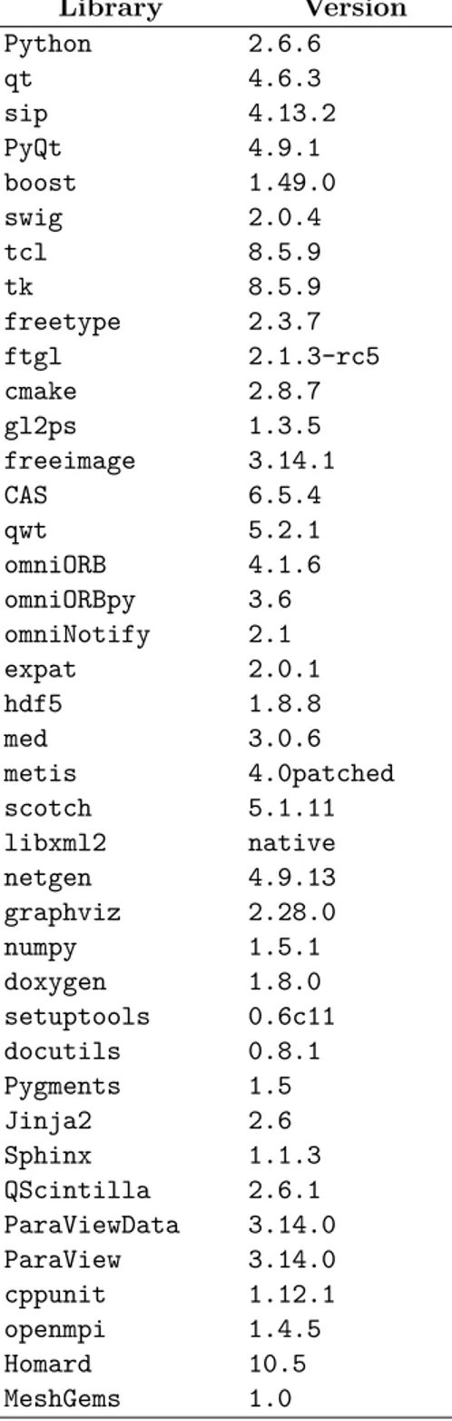
A list of the prerequisite third-party libraries that are used with v6.6.0 (developed specifically for the NURESAFE partners) is shown in Table 1.2.
Library Version Python 2.6.6 qt 4.6.3 sip 4.13.2 PyQt 4.9.1 boost 1.49.0 swig 2.0.4 tcl 8.5.9 tk 8.5.9 freetype 2.3.7 ftgl 2.1.3-rc5 cmake 2.8.7 gl2ps 1.3.5 freeimage 3.14.1 CAS 6.5.4 qwt 5.2.1 omniORB 4.1.6 omniORBpy 3.6 omniNotify 2.1 expat 2.0.1 hdf5 1.8.8 med 3.0.6 metis 4.0patched scotch 5.1.11 libxml2 native netgen 4.9.13 graphviz 2.28.0 numpy 1.5.1 doxygen 1.8.0 setuptools 0.6c11 docutils 0.8.1 Pygments 1.5 Jinja2 2.6 Sphinx 1.1.3 QScintilla 2.6.1 ParaViewData 3.14.0 ParaView 3.14.0 cppunit 1.12.1 openmpi 1.4.5 Homard 10.5 MeshGems 1.0
2 FEMLCORE coupling on SALOME
In the previous chapter we have seen the integration of the libMesh and the FEMus libraries on the SALOME platform. We have constructed interface classes (named
LIBMESH and FEMUS, respectively) that allow us to transfer data to and from the
code library to the SALOME MEDMem library. In this way by using a common com-putational platform a solution computed from a code can be transferred to another code through these interfaces. This is an ideal situation for multiscale analysis of LF reactors. The main idea is to use mono-dimensional codes to compute the primary loop evolution and three-dimensional codes to simulate in details parts of the nuclear plant. In order to do this the three-dimensional modules developed in the FEMLCORE project are there-fore coupled with mono-dimensional module created in libMesh or with any other code available on the SALOME platform. Since high specialized system codes for nuclear reactor are not open-source in this report we describe the coupling with libMesh codes in order to reach the final purpose to couple FEMLCORE with CATHARE when this code will be available on SALOME platform with an appropriate license.
In this chapter we report coupling simulations on SALOME platform based on the integration described in the previous chapter. The first section introduces libMesh cou-pling and the second section FEMus coucou-pling. Finally, in the third section, examples of FEMLCORE coupling with a mono-dimensional code developed with libMesh library are reported.
2.1 Coupling libMesh modules on SALOME
2.1.1 LibMesh energy problem coupling (3D-3D)
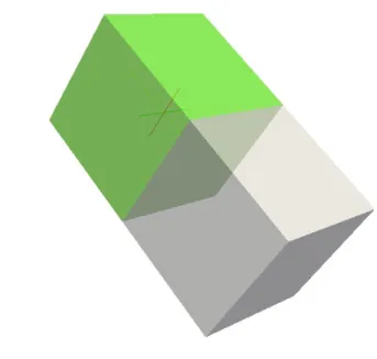
In order to verify the data transfer during the coupling with libMesh codes we consider a first simple example with the energy equation over the geometry shown in Figure 2.1.
The domain consists of two cubes: one in the region [0, 1] × [0, 1] × [−1, 0] (Ω1) and
another in [0, 1] × [0, 1] × [0, 1] (Ω2). The two meshes are created in a separate way
and the common face has the same number of points but different numbering. Each mesh consists of 12 × 12 × 12 HEX20 quadratic elements. By using GEOM and SMESH modules we have marked the boundary of the domain as up_down and down_down in the z direction, left_down and right_down in the x direction and bottom_down and
share in the y direction for the down region Ω1. The same labels is used for the up-region
(Ω2) by substituting down with up. The share region which is the common interface is
labeled share in both domains.
Over this domain we consider a problem described by the energy equation with con-stant velocity field of v = (0, 1., 0). The boundary has homogeneous Dirichlet boundary
Figure 2.1: Coupling 3D-3D geometry. Domain Ω1∪ Ω2.
condition on the up, down, left and right faces. On the share face we set homogeneous Neumann boundary conditions in the down problem and non homogeneous boundary conditions in the up region which transfers the field computed in the down problem. The
Bottom_down gets a constant field from the MEDMem interface while the top up has
homogeneous Neumann boundary conditions. We start in parallel two different prob-lems: one in the down-region and another in the up-region and continuously transfer data from the down to the top region. The LibMesh code runs through the LIBMESH class with the following code lines
LIBMESH P; LIBMESH P1; P.setType("convdiff"); P1.setType("convdiff"); P.setMesh(dataFile); P1.setMesh(dataFile1); P.setAnalyticSource("0."); P1.setAnalyticSource("0."); getInput(P, boundary); for(int itime=0;itime<60;itime++){
for(int i=0; i<boundary.size(); i++) { // boundary problem P sBC & b = boundary[i];
if(b.isAnalytic)
P.setAnalyticBoundaryValues(b.name, b.type, b.equation); else
P.setFieldBoundaryValues(b.name, b.type, b.field); }
P.solve();
getInput1(P1, P, boundary1);
for(int i=0; i<boundary1.size(); i++) { // boundary problem P1 sBC & b1 = boundary1[i];
if(b1.isAnalytic)
P1.setAnalyticBoundaryValues(b1.name, b1.type, b1.equation); else
P1.setFieldBoundaryValues(b1.name, b1.type, b1.field); } P1.solve(); sol = P.getOutputField("u"); sol1 = P1.getOutputField("u"); } P.terminate(); P1.terminate();
The LibMesh problems P and P1 are constructed in the first line. Each constructor starts its MPI boot. The problem type (convdiff) is set with setType function. The mesh with med format is assigned with setMesh function which transfers automatically the mesh to the LibMesh program. We have two meshes inside which are read from
dataFile and datafile1 respectively. The interface condition of the problem P are set by
the getInput function which is set by the user.
In order to set the interface condition the name of the different boundaries should be associated with the boundary conditions. The labels of the boundary regions are available with the function getBoundaryNames() in the LIBMESH class. The boundary conditions for the problem P are set as
boundary[0].name="right_down" boundary[0].type = "Dirichlet"; boundary[0].isAnalytic = true; boundary[0].field = NULL; boundary[0].equation = "0."; .... .... boundary[4].name="Bottom_down" boundary[4].type = "Dirichlet"; boundary[4].isAnalytic = true; boundary[4].field = NULL; boundary[4].equation = "1."; boundary[5].name="share" boundary[5].type = "Neumann";