UNIVERSITÀ DEGLI STUDI DI CATANIA
Dipartimento di Scienze Biologiche, Geologiche e Ambientali,
Sezione Scienze della Terra
D
OTTORATO
DI
R
ICERCA
IN
G
EODINAMICA
E
S
ISMOTETTONICA
XXV
CICLO
INSIGHTS INTO
ERUPTION DYNAMICS AND
SHALLOW PLUMBING SYSTEM OF MT. ETNA BY
INFRASOUND AND SEISMIC SIGNALS
Dott.ssa Mariangela Sciotto
Coordinatore
Prof. Carmelo Monaco
Tutor Co-tutor
Prof. Stefano Gresta Dott. Andrea Cannata
Dott. Eugenio Privitera
INDEX
PREFACE ... 1 1. INTRODUCTION ... 2 1.1. Volcano monitoring ... 2 1.2. Seismo-volcanic signals ... 3 1.3. Mt. Etna volcano ... 81.4. Organization of the thesis ... 12
2. ACOUSTIC WAVES ... 13
2.1. Infrasound waves in volcanic area ... 13
2.1.1. Infrasound at Mt. Etna ... 18
2.2. Acoustic wave speed in atmosphere and into the conduit ... 18
2.3. Volcano acoustic source modelling ... 20
2.3.1. Pipe resonance ... 20
2.3.2. Helmholtz resonance ... 21
3. METHODS OF ANALYSIS ... 24
3.1. Triggering algorithm ... 24
3.2. Spectral analyses ... 24
3.2.1. Fast Fourier Transform ... 25
3.2.2. Short Time Fourier Transform ... 26
3.2.3. Sompi analysis ... 28
3.2.4. Coherence analysis ... 31
3.3. Time domain analyses ... 31
3.3.1. Cross-correlation analysis ... 31
3.3.2. Subspace detector ... 33
3.4. Source location ... 36
3.4.1. Infrasound source location ... 36
3.4.2. Volcanic tremor source location ... 38
3.4.3. LP source location ... 41
3.5. Methods of analysis for seismo-acoustic signals ... 41
3.5.1. Energy partitioning analysis: Volcano Acoustic Seismic Ratio ... 41
3.5.2. Time lag estimation ... 46
4. DATASET OF ANALYSES ... 48
5. SEISMO-ACOUSTIC SIGNAL INVESTIGATIONS: CASE STUDIES ... 53
5.1. Seismo-acoustic investigations of paroxysmal activity at Mt. Etna volcano: New insights into the 16 November 2006 eruption ... 54
5.1.1. Volcanic framework ... 54
5.1.2. Data acquisition ... 56
5.1.3. Analysis of continuously acquired signals ... 57
5.1.4. Analysis of infrasound events ... 65
5.1.5. Discussion ... 73
5.1.6. Conclusions ... 81
5.2. Modelling of North-East Crater Conduit and its Relation with the Feeding System of the 2008-2009 Eruption at Mt. Etna Inferred from Seismic and Infrasound Signals ... 82
5.2.1. Volcanic framework ... 82
5.2.2. Data acquisition ... 84
5.2.3. Data analysis ... 84
5.2.4. NEC conduit model ... 93
5.2.5. Discussion ... 105
5.2.6. Concluding remarks ... 108
5.3. The 2010 ash emission at the summit craters of Mt. Etna: Relationship with seismo-acoustic signals ... 109
5.3.1. Data acquisition ... 110
5.3.2. 8 April ash emission ... 111
5.3.2.1. Volcanological data ... 111
5.3.2.2. Seismo-acoustic data analysis ... 112
5.3.3. 25 August ash emission ... 116
5.3.3.1. Volcanological data ... 116
5.3.3.2. Seismo-acoustic data analysis ... 116
5.3.4. 14-15 November ash emission ... 117
5.3.4.1. Volcanological data ... 117
5.3.4.2. Seismo-acoustic data analysis ... 117
5.3.5. Volcanic Tremor Analysis between March and December 2010 ... 118
5.3.6. Discussion and modeling ... 121
5.3.7. Concluding remarks on modeling and hazard implications ... 124
5.4. Subspace detector: lava fountain episodes at Mt. Etna volcano ... 127
5.4.2. Volcanic framework ... 128
5.4.2.1. 8-10 April 2011 eruption ... 128
5.4.2.2. 8-11 May 2011 eruption ... 129
5.4.2.3. 7-9 July 2011 eruption ... 129
5.4.3. Data analysis ... 129
5.4.4. Discussion and conclusions ... 142
6. CONCLUSIONS ... 143
ACKNOWLEDGEMENTS ... 147
REFERENCES ... 148
APPENDIX ... 171
Optimization of sensor deployment ... 171
PREFACE
The success in eruption forecasting needs the knowledge of the eruptive processes and the plumbing system of the volcano. Indeed, the eruptive styles are controlled by the interplay between magma dynamics and the plumbing system. In multi-vent volcanoes, such as Mt. Etna, where volcanic activity can rapidly vary over time and be simultaneously at the different craters, the shallow plumbing system is quite complex.
For forecasting purposes, volcano monitoring measures many geophysical parameters and interprets sub-aerial volcanic phenomena. Lots of volcanic processes occur at or near the boundary between the earth and the atmosphere, thus, beside seismic signal, acoustic waves mainly in the range of infrasound are generated. In particular, infrasound activity is usually evidence of open conduit conditions and its quantification can provide information on explosive phenomena and source mechanism. A more comprehensive knowledge of the source mechanism, as well as of the source depth into the conduit, can be achieved by exploring seismo-acoustic sources, exciting mechanical waves both in the volcano edifice and in the atmosphere.
The aim of the thesis is to look closely at the eruption dynamics at Mt. Etna, with a focus on explosive activity, and at the shallow plumbing system by means of analysis of infrasound and seismo-acoustic signals.
1. INTRODUCTION
Volcanic activity comprises a wide range of phenomena. Processes that start in the volcanic plumbing system determine the nature of subsequent events and control eruption styles (Gilbert and Lane, 2008). Beside the analysis of erupted products, one of the approaches for assessing hazard is the monitoring of the volcano. In both cases the challenge is to relate measurements made outside the volcano to active processes in inaccessible regions far below the surface (Gonnermann and Manga, 2007). Monitoring can provide insights into patterns and consequences of activity that can help draw evacuation plans. The ascent of magma in volcanoes is typically accompanied by seismicity, release of magmatic gases, and surface deformations (Sparks, 2003). Several techniques have been developed in the last decade aiming to measure these parameters and obtain useful information about state of a volcano. Nevertheless, volcanoes remain some of the most complex systems on Earth.
1.1.
Volcano monitoring
Traditional volcano monitoring techniques involve analysis of seismic signals, gas monitoring, ground deformation measurements, which in the last years are performed by means of GPS, SAR interferometry and satellite data, and magnetic and gravimetric studies. Volcanic eruptions are almost always preceded by increasing seismicity, and the most reliable indicators of impending eruption are shallow earthquakes and tremor (e.g., Chouet, 1996). Seismology gives useful information about the location of magma bodies/hydrothermal fluids in depth, their dynamics and composition and the plumbing system geometry (e.g. Kumagai and Chouet, 1999; Chouet et al., 2003; Patanè et al., 2006).
In the last decade, new insights into explosive volcanic processes have been made by studying infrasound signals (e.g., Johnson et al., 2003; Vergniolle et al., 2004; Matoza et al., 2009b). In particular, it has proved to be very useful in conjunction with seismic signal analysis (Arrowsmith et al., 2010). There is a natural synergy between seismology and infrasound not only because they share a link to some sources but also because Earth’s free surface is not an opaque boundary to either seismic or infrasonic energy (e.g., Arrowsmith et al. 2010). Such studies have provided new insights into eruption source mechanisms, by constraining the source position and obtaining quantitative information on the plume features (velocity, height and eruptive flux) (e.g. Petersen and McNutt, 2007; Caplan-Auerbach et al., 2009). In
addition, by analysing infrasound signals, inferences on the geometry of the very shallow part of plumbing systems have been made (e.g. Fee et al., 2010a; Goto and Johnson, 2011).
Other novel monitoring techniques, such as portable ground radar, which is already being deployed to document explosive eruptions and ash clouds, Muon tomography which holds promise for imaging the interior of internal structure of volcanoes (e.g. Gibert et al., 2010), and Unmanned Aerial Vehicle (UAV; e.g. McGonigle et al., 2008), may provide new monitoring capability. However, these methods will need considerable development to become widely used.
Nevertheless, the most promising method for both monitoring volcanoes and investigating their dynamics is the multiparametric approach (e.g., McNutt et al., 2000; Tilling, 2008). Recently, joint analysis of seismic, infrasonic and thermal/video signals has proved very useful in investigating explosive processes and distinguishing the different eruptive styles and dynamics in various volcanoes, such as Stromboli (Ripepe et al., 2002), Tungurahua (Johnson et al., 2005), Karymsky, (Johnson, 2007), Santiaguito (Johnson et al., 2004; Sahetapy-Engel et al., 2008), Villarica and Fuego (Marchetti et al., 2009a). Moreover, recent multiparametric approaches, based on the investigation of infrasound, several different types of seismic signals, such as earthquakes and seismo-volcanic signals, ground deformation and so on, have allowed tracking the evolution of activity in both deep and shallow parts of volcanoes (e.g., Matoza et al., 2007; Moran et al., 2008a; Di Grazia et al., 2009; Peltier et al., 2009; Aiuppa et al., 2010).
1.2.
Seismo-volcanic signals
Volcanoes are the source of a great variety of seismic signals that behave differently than those originating on tectonic earthquake faults (McNutt, 2005). Seismic signals originating from volcanoes and associated with volcanic activity are the subject of the Volcano Seismology. The variety of volcanic processes, related to magma movement at depth, and occurring during the emission at the surface of the solid, liquid, or gaseous products, may generate the seismic signals. Although earthquakes are fundamentals for tomographic studies in volcanoes, they cannot provide precise information about the location and geometry of the shallow magma conduits (Almendros et al., 2002). A more useful approach consists of investigating the seismo-volcanic signals, whose variations and features are often closely related to the eruptive activity. Indeed, they are generally considered as an indicator of the
internal state of activity of volcanoes (Neuberg, 2000). For this reason, their investigation can be very useful for both monitoring and research purposes (Patanè et al., 2011).
Therefore, the fundamentals of volcano seismology concern not only the mathematical approximation of the sources generating the seismic waves but also the description of involved magmatic processes and of the physical properties of medium where they occur (Zobin, 2012). Based on the seismo-volcanic signal nature, the main difference between earthquake and volcano seismology lies in the source mechanism and method of analyses. Following the most widely used classification in volcano seismology, seismo-volcanic signals include high frequency earthquakes, long-period and very long period events, volcanic tremor, hybrid events and volcanic explosions (McNutt, 2005; Zobin, 2012):
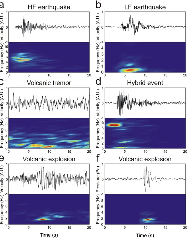
High frequency (HF) earthquakes are characterized by clear onsets of P and S waves and frequency content higher than 5 Hz (Fig. 1.1a). They are also called volcano-tectonic (VT) earthquakes since they are generated by shear fracture and are useful at volcanoes to determine stress orientation (e.g., Moran, 2003). The sources of stress causing HF events have been attributed to regional tectonic forces, gravitational loading, pore pressure effects and hydrofracturing, thermal and volumetric forces associated with magma intrusion, withdrawal, cooling, or some combinations of any or all of these (McNutt, 2005).
Long period (LP) events are characterized by dominant frequencies in the band 0.5 - 5 Hz (Chouet, 1996) (Fig. 1.1b). Features of LP events, also called low frequency (LF) events, are the emergent P wave and the lack of S waves (Chouet, 1996). LP seismic signals originating from the vibration of the stable non-destructive fluid-filled sources (dykes, conduits, cracks) carry information about the geometry of these sources and have been recorded at volcanoes during both eruptive and non-eruptive periods (Zobin, 2012 and reference therein). Investigations on the relationship between LP events and eruptions include moment tensor inversion, source location, spectral content analysis, occurrence rate, and their changes in time (e.g. Patanè et al., 2008; Cannata et al., 2009a; De Barros et al., 2009). Among the models invoked to explain source mechanism of LP events, the most accepted are the fluid-filled resonators, as cracks, conduits or spherical cavities, flow induced oscillations and bubble dynamics (Kawakatsu and Yamamoto, 2007 and reference therein). A peculiar type of LP events are the tornillos (Zobin, 2012), characterized by slowly decaying coda waves. These
signals have been recorded at different volcanoes worldwide during various stages of volcanic activity (e.g., Gomez and Torres, 1997; Milluzzo et al., 2010).
Very Long Period (VLP) events are characterized by dominant periods in the range 2-100 s (Neuberg et al., 1994; Ohminato et al., 1998) and are assumed to be linked to mass movements, and to represent inertial forces resulting from perturbations in the flow of magma and gases through conduits (Cannata et al. 2009a and reference therein). They have been recorded at many volcanoes, such as Stromboli (Neuberg et al., 1994; Chouet et al., 2003), Popocatépetl (Chouet et al., 2005), Kilauea (Ohminato et al., 1998) and Etna (Cannata et al., 2009a). Seismo-volcanic signals with period longer than 100s are named by some authors Ultra Long Period events (ULP; e.g. Ohminato et al., 1998; Houlie and Montagner, 2007).
Volcanic tremor consists of a continuous record of monotonic (harmonic) or nonharmonic vibrations that may continue for minutes to months (Zobin, 2012) and is recorded at nearly every volcano during different activity stages. Volcanic tremor has onsets emergent or impulsive, and shares the same frequency band as the LP events but has a different duration in time (Fig. 1.1c). The main features of volcanic tremor are (Konstantinou and Schlindwein, 2002): spectra consisting of a series of sharp peaks, representing either a fundamental frequency and its harmonics, or a random distribution, which exhibits temporal variations; strongly variable depths of the source, depending on the volcano, in the range of a few hundred meteres to 40 km; it may occur prior to, during and/or after eruptions. Many authors have suggested that tremor is a series of LP events occurring at intervals of few seconds (Chouet, 1992). Indeed, the models developed to explain the tremor source, generally involve complex interactions of magmatic fluids with the surrounding rocks (e.g. Kubotera, 1974; Steinberg and Steinberg, 1975; Aki et al., 1977; Chouet, 1981), and are similar to the models of LP events. A peculiar feature of seismic volcanic tremor at Mt. Etna is its continuity in time, as also observed at other basaltic volcanoes with persistent activity like Stromboli, Italy (e.g., Martini et al., 2007). Most of the energy of seismic volcanic tremor at Mt. Etna is radiated below 5 Hz (e.g., Schick and Riuscetti, 1973; Gresta et al., 1991; Cannata et al., 2008). Another interesting aspect of the seismic volcanic tremor at Mt. Etna is its close relation with eruptive activity, highlighted by variations in amplitude, spectral content, wavefield features and source location of seismic volcanic tremor at the same time as changes in volcanic activity (e.g., Gresta et al.,
1991; Alparone et al., 2007a; Patanè et al., 2008; Cannata et al., 2008, 2009b). Peculiar types of volcanic tremor are banded tremor (also observed at Etna; Cannata et al., 2010a), and gliding (phenomenon in which harmonics shift as time elapses keeping the same horizontal distance from each other; Hagerty et al., 2000). Furthermore, even acoustic radiation can appear in the shape of volcanic tremor and is therefore called infrasonic volcanic tremor (for details see section 2.1) .
Hybrid events are seismo-volcanic signals that share the waveform and the frequency content of both LP and HF events (Fig. 1.1d). These events begin with a high-frequency phase followed by a monochromatic signal similar to a LP event. Causes of hybrid events may be the mixture of source mechanisms from both HF and LP, such as brittle failure on a plain intersecting a fluid body (Lahr et al., 1994) or crack nucleation and deformation and the subsequently motion of fluid through the crack network (Benson et al., 2010).
Volcanic explosions or explosion-quakes are signals easily identifiable since they are recorded during explosive eruptions (Fig. 1.1e) and are usually accompanied by the occurrence of an air wave (Fig. 1.1f) generated by the gas release at the vent. On the other hand, it is very difficult to describe them from a seismological point of view, since they may have different features depending on the volcano, particularly conduit geometry and magma composition. Explosion-quakes may occur as a single event or as an earthquake sequence. Studying explosion earthquake at Sakurajima volcano, Uhira and Takeo (1994) demonstrated that an explosive and implosive cylindrical moment tensor component at the source depth is the dominating source mechanism for the explosion-quakes. Acoustic sensors and studies of infrasound signals have greatly improved the knowledge of volcanic explosions as will be discussed further on. Explosion earthquakes are studied with reference to their source depth and the coupling of energy between the ground and the atmosphere, and therefore the seismic and acoustic efficiency (McNutt, 2005).
Fig. 1.1 Examples of seismo-volcanic signals at Mt. Etna: (a) HF earthquake, (b) LF
earthquake, (c) volcanic tremor, (d) hybrid event, (e) seismic and (f) infrasound trace of Volcanic Explosion. From Cannata (2009).
1.3.
Mt. Etna volcano
Mt. Etna is a 3330 m high composite Quaternary volcano and lies in a complex regional setting. The volcano is located at the intersection between the front of the Appenine-Maghrebian Chain and the NNW–SSE Malta escarpment fault belt (Fig. 1.2; Barreca et al., 2012 and reference therein), which is the south-western continental margin of a Mesozoic basin of oceanic nature and extends northward with the Messina-Giardini fault zone (Doglioni et al., 2001 and reference therein). Indeed, at N and W it lies on the sediments of the chain and the E and S sectors on the Quaternary foredeep deposit of the Iblean foreland, belonging to the Pelagian block, the northernmost part of the African plate. Apart from deformations associated with uprising magma (Cocina et al., 1998), structural and seismic data indicate that the regional deformation in the Etnean area is generally dominated by N-S compression and on the eastern side by E-W extension concentrated along the Malta fault system, both offshore and onshore (Doglioni et al., 2001).
The origin of Mt. Etna has been ascribed to the tectonic control, even if an interpretation invoking an hot spot exists (Tanguy et al., 1997). Monaco et al. (1997) related the magmatism of Mt. Etna to the dilation strain on the footwall of an east-facing normal fault in the Siculo-Calabrian rift zone.
According to other authors magma uprising will be favoured by the coexistence of three main fault zones, trending ENE, NNW and WNW (Ritmann, 1973; Cristofolini et al., 1979; Lo Giudice et al., 1982). Nevertheless, recent studies invoke the south-eastward subduction rollback of the Ionian lithosphere with respect to the Hyblean plateau, along the Malta escarpement, as the cause of the development of the volcano (Gvirtzman and Nur, 1999; Doglioni et al., 2001). In particular, according to Doglioni et al. (2001) this mechanism would have generated a sort of vertical “slab window” causing the decompression and melting of magma. Furthermore, several authors have acknowledged the role of the instability of eastern flanks of the volcano on the dynamic processes on Etna (e.g. Borgia et al., 2000; Rust et al., 2005). Geophysical studies, among which GPS and SAR, revealed a continuous eastward to south-eastward motion of part of the eastern sector of the volcano (Palano et al., 2008 and reference therein). This sliding motion may cause the decompression of the plumbing system, facilitating the ascent of magma to the surface (Branca et al, 2003; Neri et al., 2004). Nevertheless, this topic is still open to debate, and several measures about the depths and the geometry of the sliding sector and interpretations dealing with the cause-effect eruption dynamics exist (Lo Giudice and Rasà, 1992; Borgia et al., 1992; Rust and Neri, 1996;
Bousquet and Lanzafame, 2001; Palano et al., 2008; Bonforte et al., 2011; Apuani et al., 2012).
Fig. 1.2 Structural setting of central Mediterranean Sea and location of Mt. Etna. 1) Regional
overthrust of the Sardinia-Corsica block upon Calabride units; 2) Regional overthrust of the Kabilo-Calabride units upon the Apennine-Maghrebian Chain; 3) External front of the Apennine-Maghrebian Chain upon the Foreland units and the External Thrust System; 4) Thrust front of the External Thrust System; 5) Main normal and strike-slip faults. KCC: Kabilo-Calabride Chain Units; AMC: Appennine-Maghrebian Chain Units; ETF: External Thrust System Units; PBF: Pelagian Block Foreland Units; QV: Quaternary Volcanoes. From Patanè et al. (2011) redrawn from Lentini et al. (2006).
The volcanism of Etna evolved from submarine and subaerial activity along regional fissures (500–200 ka) to the successive development of numerous vents dispersed over a wide area (Falsaperla et al., 2010 and reference therein). The present volcanic center is the result of two westward shifts of the plumbing system, that occurred about 130 ka and 60 ka ago together to the change of volcanism type to a central one (Branca et al., 2007, De Beni et al, 2011). About 15 ka ago a large summit caldera formed (Coltelli et al., 2000) and during the Holocene, the resuming of the eruptive activity inside the caldera built the volcanic succession of the present active volcanic center (Branca et al., 2004).
Currently, there are five active craters at the summit area of Mt. Etna: Voragine, Bocca Nuova, North-East Crater, South-East Crater and the New South-East Crater, which is a
pit-crater built on the eastern flank of South-East Crater during 2011 (hereafter referred to as VOR, BN, NEC, SEC and NSEC, respectively; see Fig. 1.3).
Fig. 1.3 Digital elevation model of Mt. Etna. In the left inset, the digital elevation model of the
summit area with the five summit craters (VOR= Voragine; BN= Bocca Nuova; NEC= North-East Crater; SEC= South-North-East Crater; NSEC= New South-North-East Crater).
These craters are characterized by persistent activity which consists of continuous degassing from vents or fumaroles on the walls of the crater, sometimes producing juvenile or lithic ash emission, and from weak to violent Strombolian explosions and short-lived lava fountains. These last volcanic phenomena are usually accompanied by the emission of lava flows. Alongside summit eruptive activity, which also includes lava flows originating from eruptive fissures opened on the flanks of the summit cones (Andronico et Lodato 2005), flank eruptions periodically occur (occurrence rate interval can vary from a few months to several decades; Allard et al., 2006). These types of eruptions take place on fissures on the slopes of the volcanic edifice and are related to the central conduit system (Andronico and Lodato, 2005). Rare eruptions, occurring on the flanks of the volcano in which magma rise throughout vertical dikes (Acocella and Neri, 2003), rather than following the central conduit path, are named peripheral eruptions.
As regarding the plumbing system of Etna, several studies of seismo-volcanic signals (for the shallowest portion) and tomographic analysis (for the intermediate portion) have been carried out in order to define its structure. Literature data agree that there is no evidence of a large magma reservoir in the crust below the volcano (Patanè et al., 2011 and reference therein). On the other hand, an high-velocity body (HVB), at a depth of 10 km beneath the Central Crater
area and the south-eastern flank of the volcano, has been recognized (Aloisi et al., 2002; Patanè et al., 2006). This has been interpreted as a large volume of non-erupted volcanic material and represents the deepest portion of the plumbing system. In the upper and lower crust seismic tomography revealed a complex high Vp body representing the old shallow
plumbing system and solified magma chambers (Patanè et al., 2011).
During an eruption, activity can be of different and sometimes simultaneous types at the different vents on Etna suggesting a quite complex shallow plumbing system. This portion of the plumbing system is studied by means of the analysis and location of seismo-volcanic signals, rather than by seismic tomography. The reason lies in resolution of tomographic analysis which is too low to allow identifying structure with scale sizes of the conduits or small temporary magma chamber in the shallower portion of plumbing system.
Recent analyses of seismo-volcanic signals carried out at Etna have allowed to image the geometry of the shallow plumbing system and track temporal variations of source location during an eruption (Lokmer et al., 2007a, Patanè et al., 2008; De Barros et al., 2009). Source locations of volcanic tremor in the time period including two lava fountains (4-5 September and 23-24 November 2007 at SEC) have evidenced two connected dike-like bodies oriented NNW-SSE and NW-SE extending from sea level to the surface, the shallower of which crossing the central craters (Patanè et al., 2008). The results of these authors are in agreement with the crack-like structure individuated by Lokmer et al. (2007a) by performing the moment-tensor inversion of LP events collected on Etna during 2004. Indeed, the hypothesized crack is centered at about 500 m below the summit, strikes in NNW-SSE direction and has an inclination from the vertical of about 20° toward the WNW (Lokmer et al., 2007a). Furthermore, De Barros et al. (2009) locating two families of LP events recorded during 2008 eruption obtained the geometry of the structure in which they are generated and move. The geometry depicted consists of a deeper planar structure which at 300 m below the summit craters splits into two branches. The authors identified the deeper structure with the dike-like body found by Patanè et al. (2008) and Lokmer et al. (2007a). The LP events have been associated to magma or gas dynamics into conduit leading to the summit craters (De Barros et al., 2009).
Moreover, further indications about shallow plumbing system geometry and the relation among conduits of the summit craters come from investigation of volcanic gas emission and petrological studies of the erupted volcanics (Burton et al., 2003; Corsaro and Pompilio, 2004; Corsaro et al., 2007, 2012; La Spina et al., 2010).
1.4.
Organization of the thesis
The present thesis is structured in six chapters and an appendix.
Chapter 1 consists of an introduction about volcano monitoring, focusing on volcano seismology, and the description of geodynamic setting and eruptive features of Mt. Etna. Chapter 2 introduces acoustics in order to define infrasound waves and in particular the different types of infrasound signals recorded in volcanic areas. This chapter also includes infrasound activity at Mt. Etna, acoustic wave speed, and detailed description of resonance models generating this kind of signal.
Chapter 3 summarizes the methods of analysis of both infrasound and seismo-acoustic signals in frequency and time domain used in the thesis.
Before describing case studies, a description of eruptive activity of Mt. Etna during the last few years is given in Chapter 4.
Chapter 5 deals with data analysis of selected eruptive episodes with the aim of characterizing both explosive dynamics and shallow plumbing system. In particular, infrasound signal recorded during the 16 November 2006 paroxysmal activity has been analysed and compared with seismic signal. The second dataset consists of seismo-acoustic events collected during 12-13 May, before the 2008-2009 eruption: features of signal and their temporal variation are analysed in order to investigate the shallower portion of plumbing system and magma dynamics therein. Furthermore, relation between infrasound and seismic energy radiated during three minor ash emissions taking place during 2010 is explored, the last section of Chapter 5 presents the application of subspace detector on infrasound data recorded during 3 lava fountains of 2011.
Chapter 6 summarizes the main results obtained.
Finally, the Appendix deals with a synthetic test aiming to the optimization of sensor deployment based on an infrasound monitoring experiment, carried out in a geothermal area of Yellowstone National Park.
2. ACOUSTIC WAVES
Acoustic waves are accountable not only for the sound that humans can hear, but also for the inaudible one. Indeed, acoustic waves can be divided into three types based on their frequency range: i) audible between ~20-20,000 Hz; ii) ultrasound above 20,000 Hz; and iii) infrasound below 20 Hz. At longer wavelengths (~ 300 s) acoustic-gravity waves are generated (Pierce, 1981).
Acoustic waves are produced as response to oscillatory processes. When the molecules of a fluid or solid are displaced from their normal configurations, the internal elastic restoring force, coupled with the inertia of the system, enables the medium to participate in oscillatory vibrations and generate acoustic waves (Kinsler, 1982). Once generated, acoustic energy propagates as a mechanical pressure wave through a medium. In the atmosphere, sound waves propagate within a gas, compressing and rarefying the medium and no shear waves are supported (Fee and Matoza, 2013).
A wide range of phenomena is able to generate infrasound waves, such as auroras, earthquakes, tsunamis, landslides, meteors, lightning and sprites, and oceanic-atmospheric dynamics (Hedlin et al., 2012 and reference therein). As mentioned in section 1.1, in the last decade infrasound has been widely employed next to volcano seismology signals, and a large literature about this topic exists (e.g., Johnson and Ripepe, 2011, Fee and Matoza, 2013 and reference therein).
2.1.
Infrasound waves in volcanic area
Due to the large length scales involved in volcanic processes, the majority of volcano acoustic oscillations occur at infrasonic frequencies (Fee and Matoza, 2013). The study of infrasound signal has many advantages. Indeed, despite potential atmospheric variability, over intermediate distances (<5 km) infrasound propagation is relatively simple compared to seismic propagation (Johnson, 2003). Furthermore, the relatively low acoustic attenuation in the atmosphere at these frequencies allows infrasound from large eruptions to propagate long distances and to be recorded globally (Fee and Matoza, 2013).
Pressure sensors, as for example microphones, record infrasonic pressure traces, which represent the time history of atmospheric pressure perturbations relative to background atmospheric pressure. This excess pressure is usually very small compared to ambient
atmospheric pressure. Thus, most of volcanic infrasonic signals can be treated as linear elastic waves rather than nonlinear shock waves (Zobin, 2012).
Analysis of infrasound signal generated by volcanoes has mainly been used for three aims: i) to understand the eruption dynamics (which includes location of infrasound sources, quantification of the outflux of volcanic materials, imaging of the very shallow portion of the plumbing system); ii) monitoring of restless volcanoes in order to assess and mitigate hazards; iii) probing of the atmosphere (Johnson and Ripepe, 2011 and reference therein). One of the advantages of infrasound monitoring is that when the efficiency of video cameras and thermal sensors is reduced (or inhibited) in the case of poor visibility due to clouds or gas plumes, it may prove a very powerful tool for the detection and characterization of explosive activity (e.g., Cannata et al., 2009b).
Arrowsmith et al. (2010), in a review of seismo-acoustic wavefield, have highlighted how the joint study of seismic and infrasound radiation provides unique constraints for studying a broad range of topics. One of these topics regards volcanic phenomena. Indeed, lots of sources relative to volcanic activity radiate energy both down into the solid Earth and up into the atmosphere (Hedlin et al., 2012). Several studies have demonstrated the usefulness of coupled seismo-acoustic investigation to constrain the position of seismo-acoustic sources inside the conduit (e.g., Ripepe et al., 2001a; Gresta et al., 2004; Kobayashi et al., 2005; Ruiz et al., 2006; Petersen and McNutt, 2007), the acoustic properties of the fluid-filled conduit (e.g., Hagerty et al., 2000), as well as to obtain a more complete model of seismo-acoustic source (e.g., Matoza et al., 2007, 2009a). Recently, seismo-acoustic studies have also been performed at Mt. Etna (e.g., Di Grazia et al., 2009).
Fee and Matoza (2013), in their review on volcano infrasound, highlighted how individual volcanoes and eruptions can exhibit multiple types of activity. Nevertheless, according to these authors, associations between eruption style and features of infrasound signals can be made.
Infrasound signals recorded in volcanic areas can be classified in explosion, jetting and infrasound tremor (Fee and Matoza, 2013):
Explosions or degassing bursts are transient events typically characterized by impulsive and compressional onset, followed by rarefaction. They can exhibit a coda lasting from few seconds to minutes. As addressed in section 1.2, volcanic explosions have a wide variety of characteristics and at times complicated source-time functions. They are commonly associated with Strombolian and Vulcanian eruptions but can occur during nearly every type of activity such as degassing activity (Fee and Matoza,
2013 and reference therein). Infrasound transients recorded in association with LP events have been ascribed to gas-release mechanism (Petersen and McNutt, 2007) or to the trigger mechanism initiating LP resonance (Matoza et al., 2009a).
Jetting is a broadband infrasound signal accompanying sustained volcanic explosions. Jetting signal observed at Tungurahua volcano by Ruiz et al. (2006) was characterized by waveforms with emergent onset and long duration codas. Based on the similarity with man-made jet noise, this kind of infrasound signal has been attributed to turbulence processes (Matoza et al., 2009b). Fee et al. (2010b) observed a low-frequency jetting during Plinian activity and pyroclastic density flow at Tungurahua. Infrasonic tremor is defined as a low frequency (<10 Hz) continuous vibration of the
atmosphere lasting from seconds to months. This kind of signal has been recorded at several volcanoes (e.g., Arenal, Garcés et al., 1998; Kilauea, Garcés et al., 2003, Fee et al., 2010a; Sakurajima, Morrissey et al. 2008; Mount St. Helens and Tungurahaua, Matoza et al., 2009a, b; Villarica, Ripepe et al., 2010). Similarly to volcanic tremor (see section 1.2.), several types of infrasonic tremor exist. Based on frequency and time domain features, harmonic, monochromatic, and broadband tremor can be distinguished. Harmonic tremor includes chugging, which is a tremor accompanied by audible pulses and is characterized by spectra with a fundamental peak at around 1 Hz and integer overtones. It has been interpreted as a succession of pressure pulses at the surface (Lees and Ruiz, 2008) and attributed to resonance of fluid-filled conduit (Garces, 2000). Furthermore, spasmodic tremor, characterized by amplitude variations, episodic tremor (bursts of tremor separated in time) and gliding (with time variations of spectral peaks) can be observed (Fee and Matoza, 2013 and reference therein). Infrasonic tremor is usually associated with lava fountain activity (e.g. Cannata et al., 2009b), and persistent effusive degassing (Matoza et al., 2010).
On the other hand, if we want to classify infrasound transients based on frequency content, and follow the nomenclature of seismo-volcanic signals, we have (Fee et al., 2010a): Infrasonic Short Period (ISP; 1-10 Hz), Infrasonic Long Period (ILP; 0.1-1 Hz), Infrasonic Very Long Period (IVLP; 0.03-0.1 Hz).
In a volcanic environment, several phenomena are able to generate infrasound signals such as rockfalls (Moran et al., 2008b) or pyroclastic flows (Oshima and Maekawa, 2001). Moreover, in a system consisting of a conduit filled with magma and gas many source mechanisms can be responsible of infrasound wave radiations, like the sudden uncorking of the volcano (Johnson and Lees, 2000), the oscillation of bubbles at the surface of a lava lake (e.g. Bouche
et al., 2010), the swelling–up of the lava plug (Yokoo et al., 2009), degassing phenomena (e.g. Fee et al., 2010a), lava fountaining and Strombolian activity (e.g. Cannata et al., 2009b), the opening of “valves” sealing fluid-filled cracks (Matoza et al., 2009a), gravity-driven bubble column dynamics responsible for conduit convection (Ripepe et al., 2010), bubble cloud oscillations in a roiling lava body and interaction of the escaping stream of gas with the vent and near-surface cavities (Matoza et al., 2010). Processes associated to magma-fluid dynamics, generating both infrasonic tremor and transients, have been modeled also invoking resonance phenomena of cavity-conduit (e.g., Garces and McNutt, 1997; Fee et al., 2010a; Goto and Johnson, 2011) and resonating gas bubbles (e.g., Vergniolle and Brandeis, 1996; Vergniolle and Caplan-Auerbach, 2004; Vergniolle et al., 2004; Kobayashi et al., 2010). Few examples of infrasound signals recorded at several volcanoes are reported in Fig. 2.1.
Fig. 2.1 Examples of 3-minute long infrasound waveforms and the relative spectrograms at
several volcanoes: pyroclastic-laden explosions from a dome at Santiaguito (A), chugging at Reventador (B), degassing from an open magma column at Kilauea (C), infrasonic tremor due to degassing from a roiling lava lake at Villarrica (D), infrasound explosions from Strombolian activity at Fuego (E) and Vulcanian ash-rich eruptions at Tungurahua (F). Cumulative energies (red lines) and power spectra (on the right) for each signal are also shown. From Johnson and Ripepe (2011).
2.1.1. Infrasound at Mt. Etna
Since 2006, the Istituto Nazionale di Geofisica e Vulcanologia (INGV), Osservatorio Etneo– Sezione di Catania, has been recording and studying the infrasound signal at Mt. Etna by a permanent network. Before the deploying of the permanent network infrasound investigations at Mt. Etna were carried out during temporary experiments (e.g. Ripepe et al., 2001b; Gresta et al., 2004).
Infrasound signals at Mt. Etna generally consist of amplitude transients, with variable duration (from 1 to a few tens of seconds), impulsive compression onsets and peaked spectra with most energy in the frequency range 1–5 Hz (Cannata et al., 2009b, c; Montalto et al., 2010). Such infrasonic signal features are similar to those observed at several volcanoes, though characterized by different volcanic activity, such as Santiaguito (Sahetapy-Engel et al., 2008), Stromboli (Ripepe et al., 1996; Marchetti et al., 2008), Tungurahua (Ruiz et al., 2006), Klyuchevskoj (Firstov and Kravchenko, 1996), Erebus (Rowe et al., 2000), Arenal (Hagerty et al., 2000), Sangay and Karymsky (Johnson and Lees, 2000). In addition, at Mt. Etna infrasonic volcanic tremor has been recorded in association with lava fountain episodes and seismic banded tremor activity (Cannata et al., 2009b, 2010a). Four summit craters have been recognized as active from the infrasonic point of view (Cannata et al., 2009b, c): NEC, BN, SEC and NSEC (the new pit-crater built on the eastern flank of the SEC cone). Infrasound radiation from these vents can be classified into continuous and sporadic activity. The former consists of short-duration releases of pressure bursts constantly generated by NEC and related to degassing activity (Cannata et al., 2009c), while the latter occurs solely during explosive activity (Strombolian explosions, lava fountains, ash emissions).
2.2.
Acoustic wave speed in atmosphere and into the conduit
In facing the study of infrasound waves in volcanic area, the acoustic speed has to be taken into account. Indeed, infrasound waves, once generated, travel into the conduit, and in the atmosphere at high altitudes, and can propagate for several kilometers before reaching the microphone. Thus, they pass through different ambient conditions, which affect their propagation.
The acoustic speed of an ideal gas, characterised by a certain chemical composition, is given by:
T R γ
cmixt mixt mixt (2.1)
where γmixt and Rmixt are the heat capacity ratio and the constant for the gas mixture,
respectively. The heat capacity ratio for a gas mixture (γmixt) is given by:
) 1 ( ) 1 (
i i i i i mixt γ X γ γ X γ (2.2)where Xi and γi are the mass fraction and the heat capacity ratio of the i-component,
respectively (Rienstra and Hirschberg, 2012). At the same way, Rmixt is defined by the sum of
the constant of the gas components (Ri). Equation 2.1 shows how cmixt for a given gas
depends on the temperature (T) and the gases composing the mixture. For example, acoustic waves in the lower atmosphere propagate with speed of 306 m/s at -40° C, 355 m/s at 40° C (Johnson, 2003), and 344 m/s at 20° C in dry air.
The estimation of acoustic speed in conduit is more difficult, since in most cases the exact values of T and gas components are unknown. Nevertheless, measures of these parameters are present in literature. For instance, Sahetapy-Engel et al. (2008) and Weill et al. (1992) considered a fluid temperature in the conduit of 1173° K for both Stromboli and Santiaguito. Fee et al. (2010a) by means of FLIR imagery estimated an average temperature inside the cavity of Halema’uma’u of about 470° K. Other authors also performed some measurements of lava temperature by FLIR, obtaining for instance ~1100-1200° K at Stromboli (Harris et al., 2005) and ~1000-1300° K at Etna (Bailey et al., 2006).
With the aim of constraining the acoustic speed in the conduit at Mt. Etna, we used chemical compositions of gas emitted by NEC during 2008 and 2009 (La Spina et al., 2010), and applied the ideal mixing theory, as reported in Morrissey and Chouet (2001). Acoustic speeds were calculated by considering temperatures equal to 300°, 800° and 1200° K and the associated Rmixt and γmixt values. In particular, for each gas specie, the Ri and γi values at 300°
K were found in Serway and Jewett (2006) and at 800° and 1200° K in Morrissey and Chouet (2001).
Therefore, applying equations 2.1 and 2.2, we obtained an acoustic speed ranging between 400 and 750 m/s.
2.3.
Volcano acoustic source modelling
Since in this thesis the analyzed infrasonic signals are interpreted as resulting from resonance phenomena related to the conduit, in the following section such phenomena will be addressed. Resonance is a propagation path effect inside the conduit and is generated by multiple reflections of pressure disturbances in the fluid against boundaries (e.g. Garces and McNutt, 1997; De Angelis and McNutt, 2007). A conduit can act as an acoustic resonator to an excitation source.
2.3.1. Pipe resonance
If the cross-sectional dimensions of a resonator are much smaller than the acoustic wavelength, the excited sound field develops a spatial variation only along the length of the resonator, i.e., longitudinal modes of the pipe are dominant and the effects of small variations in the radius are negligible (Kinsler et al., 1982). Thus, a narrow conduit can be regarded as an one-dimensional acoustic resonator. In the standing wave modes the acoustic pressure waves in the cavity volume will create a steady pattern consisting of a fixed number of sinusoidal waves between opposite cavity boundaries (Jong and Bijl, 2010). The frequencies for a closed-closed or open-open pipe resonator are equal to:
L c m f c 2 (2.3)
where cc is the acoustic speed of fluid into the conduit, m is the longitudinal mode number (m
= 1, 2, 3,…) and L is the resonating conduit portion length. For an open-closed pipe the possible frequencies are:
L c m f c 2 ) 2 1 ( (2.4)
Open-open or closed-closed conduits are characterized by spectra with peaks consisting of the fundamental mode fo (fo = cc/2L) and integer harmonics which are multiples of fo (fn = m fo),
while open-closed conduit conditions generate the fundamental frequency and odd harmonics (fn = (m - 1/2) fo) (De Angelis and McNutt, 2007). The relevant parameters in the pipe
impedance of the conduit terminations may indicate changes in the cross-sectional area of the conduit and/or changes in the density and sound speed of the fluid filling the conduit (Graces and McNutt, 1997). In order to state if a termination is closed or open the contrast of impedance should be taken into account. Further, the end correction has to be considered (Morse and Ingard, 1986). Physically the end correction can be understood as an effect of the mismatch between the one-dimensional acoustic field inside the pipe and the three-dimensional field outside that is radiated by the open end. The end correction for a closed end is naturally zero, while for an open end is 0.6*l (where l is the pipe radius) (Miklos et al., 2001).
Fig. 2.2 Sketch of a pipe resonator. From Raichel (2006).
2.3.2. Helmholtz resonance
Another possible excitation mechanism of volumes with a small opening is Helmholtz resonance. Helmholtz resonator is a harmonic oscillator with only one degree of freedom (volume) and is termed a lumped acoustic element (Kinsler et al., 1982). It consists of a cavity connected with the outside space through a narrow neck or through an opening (Fig. 2.3; Alster, 1972).
Fig. 2.3 Sketch of a Helmholtz resonator. From Campbell and Peatross (2011).
Helmholtz resonators do not work on the principle of formation of standing wave pattern. Instead, they can be modeled as a simple mass loaded on a spring system. The fluid in the neck acts as the mass, while the fluid pressure on both inside and out of the resonator acts as the spring. The effective mass of the fluid in the neck is given by (Kinsler et al., 1982):
'
SL ρ
m (2.5)
where ρ is the density of the fluid, S is the area of the neck (narrowing) and L' is the effective neck length. This effective neck length L' is longer than the physical length (a) because of its radiation mass loading. The air pressure acts as a spring in the system. The “spring constant” of the air pressure (stiffness) is given by (Raichel, 2006):
V S c ρ k 2 2 (2.6)
V is the cavity volume (conduit). The driving force acting on the opening is given by:
PS
F (2.7)
SP δ k dt δ d m 22 (2.8)
where δ is the displacement of the slug of air contained in the neck. Solving equation 2.8, resonance frequency is obtained:
m k
ω 0 (2.9)
Substituting in equation 2.9 m and k (equations 2.5 and 2.6, respectively) we obtain that the Helmholtz resonator frequency is equal to:
' 2 VL S π c f c (2.10)
As regarding the effective length, it takes into account the air/fluid above and below the neck region acting as inertial mass. The end correction is equal to 0.85*l if the outer opening of the neck is flanged, and 0.6*l if it is unflanged, as aforementioned. While the inner opening of the neck is assumed to be equivalent to a flanged termination (Kinsler et al., 1982). We considered the outer end of the narrowing unflanged, therefore the combination of the corrections gives:
l a
L' 1.45* (2.11) where l is the neck radius and a, as aforementioned, is the physical length of the neck. One assumption that has to be done in deriving the frequency of the Helmholtz resonator is that all dimensions of the system are much smaller than the acoustic wavelength. In the case of the lower infrasonic frequencies recorded at Etna (e.g. 0.4-0.7 Hz), wavelengths (~500-850 m), with an acoustic speed of 340 m/s, are much longer than the reasonable dimensions of the conduit.
3. METHODS OF ANALYSIS
3.1. Triggering algorithm
The analysis of seismo-volcanic events needs, as the first step, the extraction of the signal portion containing the transient from the continuous recording.
Several kinds of trigger algorithm have been developed based on the specific requirements of seismological applications. Withers et al. (1998) have categorized previous trigger algorithms for onset picking into time domain, frequency domain, particle motion processing, or matched filter.
The automatic detection of infrasound and seismic transients analyzed in this work has been performed by means of Short Time Average through Long Time Average (STA/LTA). STA/LTA is an energy detector in so far as it depends on the amplitude fluctuations of the signal. It is the most common technique in seismological study since it requires little information about the signal to be detected. Indeed, it depends on the amplitude fluctuations of seismic signal, rather than signal polarization and frequencies (Sharma et al., 2010). The algorithm first calculates the absolute amplitude of the signal, then averages the amplitudes in both the short and the long window. The short period average represents the average of the shortest period over which an event of interest could occur, while the long period average represents the average of the longest period to assess the background noise. In the next step a ratio of STA/LTA is calculated and is continuously compared to a preset threshold value. Once the ratio exceeds the threshold, the trigger is declared (Trnkcnozy, 2012).
3.2. Spectral analyses
The time and frequency domains are alternative ways of representing signals and analyses in time and frequency domain, and are complementary for the understanding of the behaviour of a dynamic system. Time domain analysis allows to study variations in time of parameters like for example the shape or the amplitude of the signal waveform. In the frequency domain the signal is represented as decomposed in sinusoidal components. Most signals and processes involve both fast and slow components happening at the same time. Frequency domain analysis separates these components and helps to keep track of them.
3.2.1. Fast Fourier Transform
The time and frequency domain representations are related to each other by the Fourier transform (Rauscher et al., 2001), so each signal in the time domain has a characteristic frequency spectrum:
te dt x f F( ) j 2πft
(3.1)where f is the frequency, x(t) is the signal in time domain, F(f) is the Fourier transform of x(t), and j is equal to . The calculation of the signal spectrum from the samples of the signal 1 in the time domain is referred to as a discrete Fourier transform (DFT). DFT is almost always computed in practice by Fast Fourier Transform (FFT; Cooley and Tukey, 1965), which is not a new transform, but is the most widely used algorithm for efficiently computing the DFT for applications such as spectrum analysis (Fig. 3.1).
Fig. 3.1 Infrasonic event recorded at Mt. Etna (top) and its spectrum calculated on 10.24
second-long time-window (bottom).
3.2.2. Short Time Fourier Transform
Seismic and acoustic signals are of non-stationary nature, that is, their spectral content changes over time. In this case, FFT, since it is based on the assumption of stationary behaviour of the signal, is not able to show the temporal distribution of frequencies. To become accurate in time, a frequency versus time representation of the signal is needed. This kind of spectral decomposition is provided by the Short Time Fourier Transform (STFT). By assuming that signal x(t) is stationary when seen through a small time window, then the FFT can be computed on a windowed signal. The signal is segmented by means of sliding window functions (g) of a limited extent (t) and centered in τ. The Fourier transform of the windowed signal yields to the STFT, which mathematically is defined as (Rioul and Vetterli, 1991):
dt e τ t g t x f τ STFT( , ) ( ) ( ) j 2πft
(3.2)where g* is the complex conjugate of the sliding window function. Therefore, the STFT method is able to analyze a non-stationary signal in the time domain through a segmented algorithm. A moving window process breaks up the signal into a set of segments (time windows), and each of them is processed by the FFT algorithm. The sliding window function plays an important role in the STFT, and once has been chosen, it fixes the time-frequency resolution of the analysis. If this function has a long duration in time, it implies a fine sampling of the frequency, but small changes in the time domain are obscured because of averaging. Instead, a window function of short time duration defines short-lived variations in time but has a poor frequency resolution. Due to the Heisenberg’s uncertainty principle a small time window and a narrow bandwidth window cannot exist contemporaneously, thus a trade-off window size needs to be selected according to frequency and time resolution such that the interesting features of the signal one is looking for are solved (Fig. 3.2).
Fig. 3.2 Infrasonic event recorded at Mt. Etna (top) and STFT calculated on 5.12 second-long
time-window (bottom).
3.2.3. Sompi analysis
Beside the Fourier transform, there is another type of approach for spectral analysis which implies a time series modelling based on the characteristic property of a linear dynamic system. Several seismo-volcanic signals show a clear trend of amplitude to decay with time, then the decomposition of time series into purely harmonic components (Fourier transform case) can cause a loss of information (Kumazawa et al., 1990). Various studies (Chouet, 2003 and references therein) demonstrated that in such cases spectral features will be reasonably represented in the complex frequency space, rather than in the real frequency space as in the
previous method. In particular, a method called “Sompi” has become commonly used in volcano-seismology for his high spectral resolution in determining the decay characteristics and the oscillation period of time series corrupted by noise (e.g. Kumagai and Chouet, 1999, 2000). Sompi method assumes that the observed signal is the realization of a hypothetical linear dynamic system and estimates the characteristic frequencies by determining the autoregressive model (AR) equations that best describe the system (Kumazawa et al., 1990). In practice, a given signal is decomposed into a linear combination of finite-number coherent sinusoids with amplitudes exponentially decaying (or growing) with time such as:
) ( ) cos( ) ( 1 t ε θ t ω e A t x n γt i i i i i ω
(3.3) where nω is the number of sinusoids called wave elements, ε(t) is incoherent noise and ωi, γi, Ai, θi are the real parameters characterizing each wave element. In particular, ω and γcorrespond respectively to the real and imaginary parts of the complex angular frequency (z =
exp(γ+iω)), and Ai and θi are respectively the real amplitude and the phase angle of the
complex amplitude α (α = Aеiθ). From these parameters we can extract spectral features of the
signal as the real frequency (f) and the growth rate (g) (Kumazawa et al., 1990):
π ω f 2 (3.4) π γ g 2 (3.5)
Further, the quality factor Q is related to f and g through:
g f Q 2 (3.6)
In order to apply the Sompi method a transient in a signal, composed of superposition of simple decaying sinusoids is taken into account, its onset is neglected, and the analysis is performed on the tail (grey are in Fig. 3.3a). The first step is the extraction of the wave elements from the signal, then each wave element is characterised by a set of f and g without information about excitation (amplitude and phase). Spectral analysis results of the Sompi method are usually plotted in 2D diagram with f-g axes (Fig. 3.3b). This kind of diagram
allows to identify the dominant modes (circled points in Fig. 3.3b), corresponding to the wave elements remaining mainly stable as the AR order changes, from the noise whose wave elements are scattered in the plot (Hori et al., 1989). Besides the frequency and the growth rate, another important parameter obtainable from the Sompi analysis is the quality factor Q. It can be considered a measure of the decay time of the sinusoids, thus can give information about the features of the resonator system in terms of attenuation (Chouet, 2003 and references therein).
Fig. 3.3 (a) Infrasound event recorded at Mt. Etna and corresponding (b) frequency-growth
rate plot (AR order 2–60). The dashed lines in (b) represent lines along which the quality factor (Q) is constant. Circled points in (b) indicate dominant spectral components of the signal; scattered points represent noise. From Cannata et al. (2011b).
3.2.4. Coherence analysis
In some volcanoes seismo-acoustic investigations have shown how seismic and infrasonic signals sometimes share almost the same spectral content, suggesting a common source for both the signals (e.g., Stromboli, Ripepe et al., 1996; and Kilauea, Matoza et al., 2010). The coherence function provides the correlation between two signals at a certain frequency λ. It is defined by (Saab et al., 2005):
) ( ) ( ) ( ) ( 2 YY XX XY XY P P P C (3.7)
where PXX and PYY are the autospectra of signal X and Y, respectively, and PXY is the cross
spectrum. The result is a real number between 0 and 1. This function allows to investigate the coherence between two signals over time and can be represented in 2D diagram in which x axis is the time, y axis indicates the frequency and the colour scale shows the coherence values.
3.3. Time domain analyses
3.3.1. Cross-correlation analysis
Recent applications of correlation methods to seismological problems illustrate the power of coherent signal processing applied to seismic waveforms. Examples of these application include detection of low amplitude signals buried in ambient noise and cross-correlation of sets of waveforms to form event clusters. The waveforms of earthquakes and long period events are often similar enough that waveform cross correlation can be used to detect them and obtain much more precise differential times in order to perform high-precision relocation (e.g. Lin et al., 2007, De Barros et al., 2009). Beside the relocation, given a signal template from a preciously observed event, the cross-correlation can simply detect subsequent occurrences of that signal on the incoming data (Schweitzer et al., 2011).
During a given eruptive episode hundreds or thousands of low-frequency events can occur. Often variations in the characteristics of the low-frequency events are strictly related to changes in source mechanism. In order to identify patterns and systematic changes in the signal a classification of the events in groups is very useful. Besides the spectral content, the
classification can be based on waveforms. These cross-correlation based methods rely in the quantification of the similarity of waveforms which is defined as (Green and Neuberg, 2006):
n i i n i i l n i l i i xy x x y y y y x x l i i cc 1 2 1 2 1 , (3.8)where xi is the i-th sample of the signal x, yi-l is the (i-l)-th sample of the signal y and the
overbar represents the mean value of the signal. The index l is the lag between the two signals; changing this parameter varies the relative position of signal x with respect to signal
y. Finally, n is the number of samples of the considered windows of x and y. ccxy lies in the
interval [-1,1]. Identical waveforms result in ccxy = 1; two time-series with no correlation
produce ccxy = 0; waveforms which are identical except reversed polarities generate ccxy = -1.
In the cross-correlation analysis every single event is compared with every other event of the whole dataset. Once the correlation functions are calculated, the CC matrix is built. This matrix consists of maximum correlation coefficient values between the couples of events (e.g. seismic or infrasound events) that are obtained by changing the lag between them (Fig. 3.4). For the purpose of event classification, the events need to be grouped into families. In this work, we choose the method of Green and Neuberg (2006), whose grouping approach allows to identify gradual waveform variations among the families. In this waveform classification the event with the largest number of cross-correlation value above a fixed threshold is selected and is called the “master event”. Successively, a waveform stacking is performed by averaging the waveforms of all the events well correlated with the master event. This waveform stacking is then cross-correlated with the original dataset of events, allowing to group all the events, that have cross-correlation coefficient largest than the threshold, into a family. This procedure is then repeated iteratively until the entire matrix is grouped into families. The cross-correlation threshold is chosen as a trade-off between classification accuracy and event detection, and the window length is to be fixed according to the event features.
Fig. 3.4 Example of the cross correlation matrix of infrasound events recorded at Mt. Etna.
The dashed vertical lines show the main waveform variations. From Cannata et al. (2011a).
Further more, one of the most powerful and useful output measures resulting from cross-correlation analysis is the temporal shift or lag (l) of one signal relative to the other. The lag can provide information about when signal events are happening relative to each other in each of the signals used for the cross-correlation.
3.3.2. Subspace detector
As aforementioned, the most common trigger algorithm used in seismology is the STA/LTA since it is able to detect signal with no specific characteristic and no a priori information about the events to be detected. However, a disadvantage of an energy detector, is the high false alarm rate when thresholds are set aggressively to detect smaller signals. An alternative algorithm is the matched filter, which correlates a template waveform against a continuous data stream to detect occurrences of that waveform. Cross-correlation based detectors are highly sensitive and have high probabilities of detection at low false alarm rates (Gibbons and Ringdal, 2006). They revealed to be very useful to strictly repetitive sources, but require perfect knowledge of the signal. However, repeating sources frequently produce varied waveforms not well represented by a single template (Harris, 2006). Broadband subspace detectors are introduced for seismological applications that require the detection of repetitive
sources that produce similar, yet significantly variable seismic signals (Harris, 2006). Subspace detectors operate by correlating a linear combination of a set of orthonormal basis waveforms (developed from the reference template waveforms produced by a particular source) against an incoming data stream to detect signals that lie in the subspace spanned by the basis (hence the name “subspace detector”) (Harris, 2006). Doing so, it can detect both identical events and events that exhibit small variations with respect to the reference templates. Hence, the subspace detector turns out to be powerful for the detection of explosive infrasonic events occurring in a volcanic area. Indeed, during an eruption a single crater usually produces similar but not identical infrasonic events due to temporal variation in explosion dynamics, in vent geometry or in location (e.g. two or more vents inside a single crater). Similar to other detectors, the subspace implements a binary hypothesis test on the presence or absence of a signal in a data observation window (Van Trees, 1968). The signal is assumed to be deterministic, but dependent upon a vector of unknown parameters, and is specified as an unknown linear combination of basis waveforms. The unknown signal and noise parameters are estimated from the data as a generalized likelihood ratio test. To calculate the basis, reference waveforms (templates) are organized as columns of a data matrix and a singular value decomposition (SVD) is computed (Maceira et al., 2010). The basis consists of the left singular vectors corresponding to the most significant singular values in the decomposition. The subspace detector operates by projecting the data in a detection window into a subspace spanned by the column of the subspace representation matrix (U) (Fig. 3.5).