Image quality and dose evaluation of filtered back projection versus iterative reconstruction algorithm in multislice computed tomography.

(1)

Alma Mater Studiorum · Universit`

a di Bologna

Scuola di Scienze

Corso di Laurea Magistrale in Fisica

Image Quality and Dose Evaluation

of Filtered Back Projection Versus

Iterative Reconstruction Algorithm

in Multislice Computed

Tomography

Relatore:

Prof. Maria Pia Morigi

Correlatore:

Prof. Luisa Pierotti

Presentata da:

Daniele Pesolillo

Sessione III

(2)

(3)

(4)

(5)

List of Figures

1.1 Hounsfield’s sketch (left), Lithograph of Hounsfield Original Test Lathe, presented to

the author on the late 1970s (right). . . 8

1.2 A modern CT Scanner, Philips Brilliance 64 CT Scanner.. . . 9

1.3 Sample of garnet-biotite-kyanite schist. . . 11

1.4 Gantry virtual view. . . 12

1.5 Gantry External view. . . 13

1.6 Gantry Internal view. . . 13

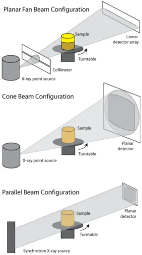
1.7 Some of the most common configurations for CT scanners. . . 16

1.8 A representation of first generation CT scanner (Parallel Beam, Translate-Rotate). . 17

1.9 A representation of second generation CT scanner (Fan Beam, Translate-Rotate). . . 18

1.10 A representation of third generation CT scanner (Fan Beam, Rotate only).. . . 19

1.11 A representation of fourth generation CT scanner (Fan Beam, stationary circular detector). . . 20

1.12 Artistic representation of axial CT. . . 21

1.13 Comparison between higher pitch and lower pitch[7]. . . 23

1.14 Artistic representation of spiral CT. . . 23

1.15 Spiral Slice Sensitivity Profile (SSP) of SSCT in Spiral Mode (LEFT); As the pitch increases, SSP curves deviate more and more from an ideal square wave (-0.5 to 0.5) more similar to conventional (non-spiral) CT. Spiral Slice Sensitivity Profile of MSCT in Spiral Mode (RIGHT); Fractional pitch of multislice leads to better approximation of SSCT, more similar to ideal square wave (-0.5 to 0.5)[1]. . . 26

1.16 SSCT arrays containing single, long elements along z-axis (Left). MSCT arrays with several rows of small detector elements (Right)[8]. . . 26

1.17 Diagrams of various 16-slice detector designs (in z-direction). Innermost elements can be used to collect 16 thin slices or linked in pairs to collect thicker slices[8]. . . 27

1.18 Diagrams of various 64-slice detector designs (in z-direction). Most designs lengthen arrays and provide all submillimeter elements. Siemens scanner uses 32 elements and dynamic-focus x-ray tube to yield 2 measurements per detector[8]. . . 27

2.1 Radon Transform. . . 29

2.2 The Shepp-Logan head phantom (left) and its Radon Transform (right). . . 30

(8)

iv LIST OF FIGURES

2.3 The Fourier slice theorem. In the spatial domain, each view is found by integrating the image along rays at a particular angle. In the frequency domain, the spectrum of

each view is a one dimensional slice of the two dimensional image spectrum. . . 33

2.4 Backprojection reconstructs an image by taking each view and smearing it along the path it was originally acquired. The resulting image is a blurry version of the correct image. . . 34

2.5 Filtered backprojection reconstructs an image by filtering each view before backpro-jection. This removes the blurring seen in simple backprojection, and results in a mathematically exact reconstruction of the image.. . . 35

2.6 The basic workflow of an FBP. . . 36

2.7 Schematic view of the iterative reconstruction process[13]. The volume estimated is initiated either with an empty image or, if available, an FBP reconstruction. If a stop criterion is matched,the loop is terminated and the current volumetric image becomes the final volumetric image. . . 36

2.8 Selection of the most prominent iterative reconstruction algorithms. . . 37

2.9 The basic workflow of an ASIR algorithm. . . 39

2.10 The basic workflow of an MBIR algorithm. . . 39

2.11 Statistical and Model-based Iterative Reconstruction Algorithms Developed by Major Computed Tomography Manufacturers[16]. . . 40

2.12 In a 15-year-old patient presenting to the emergency department to rule out appen-dicitis, low-dose scan with FBP reconstruction was noisier than follow-up imaging using the same dose with ASiR reconstruction[18]. . . 41

2.13 Liver metastasis visualized with VEO. The right image is less noisy than other[19]. . 42

2.14 Comparison between standard protocol (FBP) and Iterative reconstruction in image space [see www.healthcare.siemens.com]. . . 43

2.15 Comparison between FBP and Sinogram Reconstruction. Image noise decrease with-out loss of resolution in the right image [see www.healthcare.siemens.com]. . . 44

2.16 In the left image we see noise reduction with AIDR3D. In the right image is shown the workflow for dose reduction AIDR 3D [see toshibamedicalsystems.com]. . . 45

2.17 Image enhancement of an abdomen using IMR [see www.healthcare.philips.com]. . . 46

2.18 Summary of noise reduction and artifact prevention capabilities provided by each reconstruction generation (left). Adapting dose reduction and spatial resolution based on the clinical indication (right) [see www.healthcare.philips.com]. . . 47

3.1 Philips Phantom used for acquisition. Body phantom (LEFT SIDE) and head phan-tom (RIGHT SIDE). . . 50

3.2 Convolution kernel for body phantom. . . 52

3.3 Spatial frequency (mm−1) and radially NNPS values (mm2_{) (LEFT). Body phantom} image and ROI utilized for calculate the Normalized Noise Power Spectrum (RIGHT). 53 3.4 Values of NNPS calculate for all seven slice with FBP algorithm and Convolution kernel A. . . 53

(9)

LIST OF FIGURES v

3.5 2D image of the NNPS, note the circular symmetry. . . 54

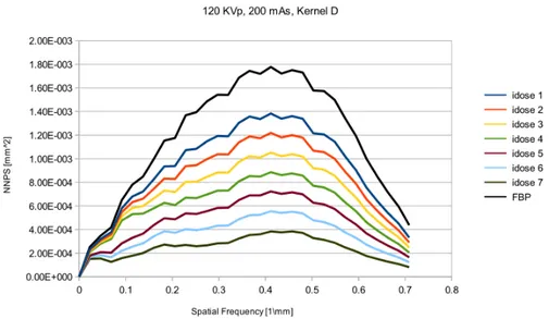
3.6 Normalized noise power spectrum for different iDose levels. An image reconstructed using this filter, producing noise texture with low spatial frequency noise. See Ap-pendix A for phantom’s image. . . 55

3.7 Normalized noise power spectrum for different iDose levels. First idose level will have two peaks while iDose6 will have one peak shifted at lower frequencies. See Appendix A for phantom’s image. . . 55

3.8 Normalized noise power spectrum for different iterative reconstruction levels. For higher levels the peaks from 0.25 mm−1 to 0.35 mm−1disappear. See Appendix A for phantom’s image. . . 56

3.9 All curves shifted by high frequencies than other kernels. See Appendix A for phan-tom’s image.. . . 57

3.10 Shape of Normalized Noise Power Spectrum of FBP and reconstruction levels. The curves tends to zero more slowly than the others filter. See Appendix A for phantom’s image. . . 58

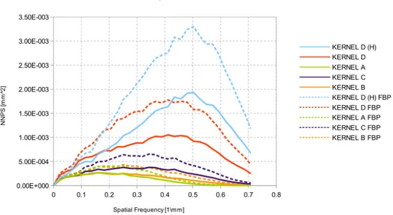
3.11 Trend of noise power spectrum for all reconstruction kernels. Radially averaged nor-malized NPS curves show how noise texture is manifested in the NPS. . . 60

3.12 Trend of noise power spectrum for all reconstruction kernels. Note the differences at ∼ 0.45 mm−1_{and ∼ 0.3 mm}−1_. _{. . . .} ₆₁

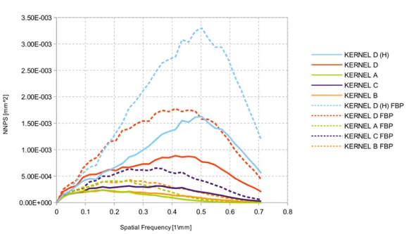
3.13 Trend of noise power spectrum for all reconstruction kernels. Note the lowest noise power for kernel D (FBP) after 0.55 mm−1. . . 63

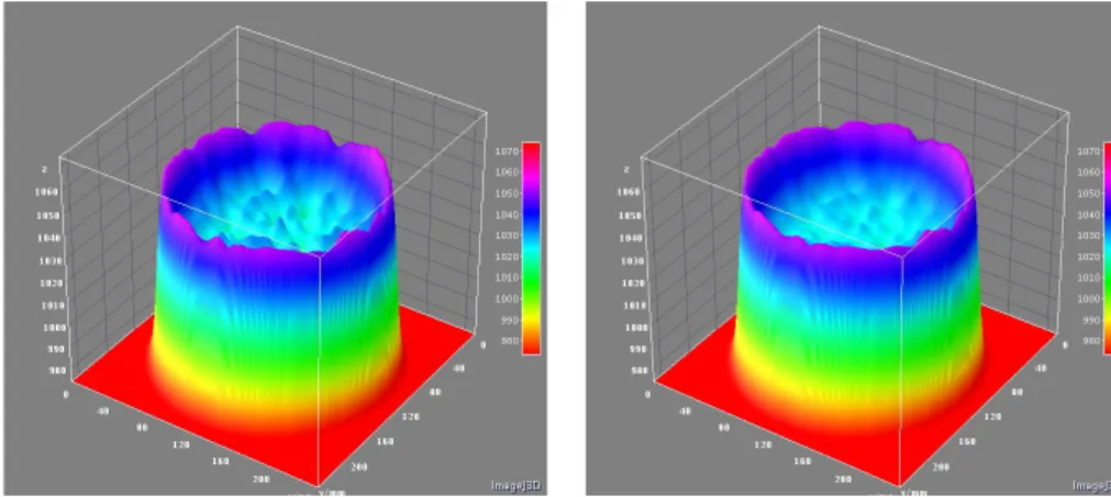
3.14 Noise texture fluctuations of Filtered Back Projection algorithm with convolution kernel A (LEFT). Noise texture fluctuations of Iterative reconstruction algorithm (iDose, level 4) with same convolution kernel of FBP (RIGHT). The teflon insert is not affected by noise texture and reconstruction algorithm. . . 64

3.15 Convolution kernel for Head Phantom. . . 65

3.16 Spatial frequency (mm−1) and radially NNPS values (mm2_{) (LEFT). Head}

phan-tom image and region of interest utilized for calculate the Normalized Noise Power Spectrum (RIGHT). . . 66

3.17 Values of NNPS calculate for all seven slice with FBP algorithm and Convolution kernel A. Note the different values of spatial frequency for head phantom compared to body phantom. . . 67

3.18 Trend of noise power spectrum for all reconstruction kernels, except kernels UB-EB. Radially averaged normalized NPS curves show how noise texture is manifested in the NPS.. . . 68

3.19 Comparison between smooth convolution kernels for head acquisition. UB improves bone-brain interface and no effect on HU values; EB head scans only and increased to observed HU values (not shown here). . . 69

3.20 Trend of noise power spectrum for all reconstruction kernels, except kernels UB-EB. Radially averaged normalized NPS curves show how noise texture is manifested in the NPS.. . . 70

(10)

vi LIST OF FIGURES

3.22 Trend of noise power spectrum for all reconstruction kernels, except kernels UB-EB. Radially averaged normalized NPS curves show how noise texture is manifested in the NPS. . . 72

3.24 Noise texture fluctuations of Filtered Back Projection algorithm with convolution kernel DH (LEFT). Noise texture fluctuations of Iterative reconstruction algorithm (iDose, level 4) with same convolution kernel of FBP (RIGHT). . . 74

3.25 (a)Input images defining the point-spread function, the line-spread function and the edge-spread function.(b) Simulated degraded-output images showing raw image data used for the measurements of the PSF, LSF and ESF. The blurring seen in these functions is due to the imperfect resolution properties of the imaging system being characterized.(c) Graphs showing the actual PSF, LSF and ESF. The PSF is a 2D function, and the LSF and ESF are 1D functions. . . 77

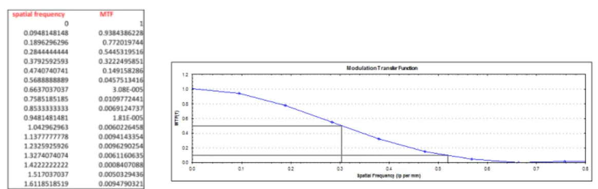
3.26 Phantom image corresponding to the Philips head phantom using a typical adult head protocol. Image window and level have been adjusted to show bead point source within the ROI (LEFT). Modulation transfer function reconstructed with kernel A; the spatial frequencies at 10% and 50% are shown (RIGHT). . . 79

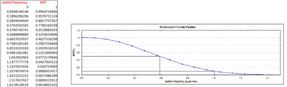
3.27 MTF values with FBP and iterative algorithm using kernel A (LEFT). MTF plot and values of spatial frequency at 10% and 50% (RIGHT.) . . . 80

3.28 MTF values with FBP and iterative algorithm using kernel EB (LEFT). MTF plot and values of spatial frequency at 10% and 50% (RIGHT.) . . . 80

3.29 MTF values with FBP and iterative algorithm using kernel UB (LEFT). MTF plot and values of spatial frequency at 10% and 50% (RIGHT.) . . . 80

3.30 MTF values with FBP and iterative algorithm using kernel C (LEFT). MTF plot and values of spatial frequency at 10% and 50% (RIGHT.) . . . 81

3.31 MTF values with FBP and iterative algorithm using kernel DH (LEFT). MTF plot and values of spatial frequency at 10% and 50% (RIGHT.) . . . 81

3.32 MTF for filtered back projection and level 1 of iterative reconstruction algorithm. . . 82

3.33 MTF for level 2, level 3 and level 4 of iterative reconstruction algorithm. . . 83

3.34 MTF for level 5 of iterative reconstruction algorithm. . . 84

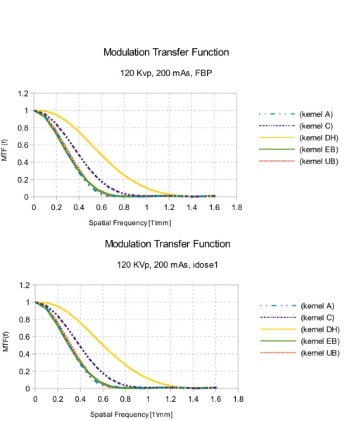
3.35 Modulation transfer function at 10% compared standard deviation for all convolution kernels. The filter DH has a value greater than other. . . 86

3.36 Modulation transfer function at 50% compared standard deviation for all convolution kernels. The filter DH has a greater value than other. . . 86

(11)

LIST OF FIGURES vii

4.1 Catphan 600 phantom (LEFT). CTP515 low contrast module with supra-slice and

subslice contrast targets (RIGHT). . . 88

4.2 Catphan phantom analysis using nominal contrast of 1%. . . 91

4.3 Contrast to noise ratio for iterative and standard algorithm. We can see the differences between the values; they are very similar between kernel UB and EB. . . 92

4.4 Trends of contrast to noise ratio at varying levels of reconstruction.. . . 93

4.5 Catphan phantom analysis using nominal contrast of 0.5%. . . 94

4.6 Contrast to noise ratio for iterative and standard algorithm. We can see the small differences between the filter C and EB. . . 95

4.8 Catphan phantom analysis using nominal contrast of 0.3%. . . 96

4.9 Contrast to noise ratio for iterative and standard algorithm. We can see the differences between the filters C, EB and UB. . . 97

4.11 Spiral CIRS phantom, internal view (LEFT). Phantom contains spherical objects; these spheres are placed in three rows. Each row contains spheres that were origi-nally designed to be 20, 10, and 5 HU below background (designed to equal liver; no attenuation given (RIGHT). . . 99

4.12 Cirs 061 phantom analysis using nominal contrast 2%. . . 101

4.13 Contrast to noise ratio for iterative and standard algorithm. . . 102

4.15 Cirs 061 phantom analysis using nominal contrast 1%. . . 103

4.18 Cirs 061 phantom analysis using nominal contrast 0.5%. . . 105

5.1 Illustration of the term ”Computed Tomography Dose Index”. . . 110

5.2 Illustration of the term ”Dose Length Product”. . . 112

5.3 Phantom kit to evaluate CTDI (LEFT) and internal view with pencil chamber (RIGHT).112 A.1 Filtered Back Projection reconstruction with kernel A (LEFT). Iterative reconstruc-tion with kernel A (RIGHT). . . 119

A.2 Filtered Back Projection reconstruction with kernel B (LEFT). Iterative reconstruc-tion with kernel B (RIGHT). . . 119

A.3 Filtered Back Projection reconstruction with kernel C (LEFT). Iterative reconstruc-tion with kernel C (RIGHT). . . 120

A.4 Filtered Back Projection reconstruction with kernel D (LEFT). Iterative reconstruc-tion with kernel D (RIGHT). . . 120

(12)

viii LIST OF FIGURES

A.5 Filtered Back Projection reconstruction with kernel DH (LEFT). Iterative reconstruc-tion with kernel DH (RIGHT). . . 120

A.6 Filtered Back Projection reconstruction with kernel A (LEFT). Iterative reconstruc-tion with kernel A (RIGHT). . . 121

A.7 Filtered Back Projection reconstruction with kernel UB (LEFT). Iterative reconstruc-tion with kernel UB (RIGHT). . . 121

A.8 Filtered Back Projection reconstruction with kernel EB (LEFT). Iterative reconstruc-tion with kernel EB (RIGHT). . . 121

A.9 Filtered Back Projection reconstruction with kernel C (LEFT). Iterative reconstruc-tion with kernel C (RIGHT). . . 122

A.10Filtered Back Projection reconstruction with kernel D (LEFT). Iterative reconstruc-tion with kernel D (RIGHT). . . 122

A.11Filtered Back Projection reconstruction with kernel DH (LEFT). Iterative reconstruc-tion with kernel DH (RIGHT). . . 122

A.12Average NNPS both Filtered Back Projection and Iterative reconstruction algorithm, head phantom. Spatial Frequency [mm−1_{], NNPS [mm}2_]. _{. . . 123}

A.13Average NNPS both Filtered Back Projection and Iterative reconstruction algorithm; body phantom. Spatial Frequency [mm−1], NNPS [mm2_]. _{. . . 123}

A.14Noise texture fluctuations of Filtered Back Projection algorithm with convolution kernel B (LEFT). Noise texture fluctuations of Iterative reconstruction algorithm (iDose, level 4) with same convolution kernel of FBP (RIGHT). The teflon insert is not affected by noise texture and reconstruction algorithm. Body phantom. . . 124

A.15Noise texture fluctuations of Filtered Back Projection algorithm with convolution kernel C (LEFT). Noise texture fluctuations of Iterative reconstruction algorithm (iDose, level 4) with same convolution kernel of FBP (RIGHT). The teflon insert is not affected by noise texture and reconstruction algorithm. Body phantom. . . 124

A.16Noise texture fluctuations of Filtered Back Projection algorithm with convolution kernel D (LEFT). Noise texture fluctuations of Iterative reconstruction algorithm (iDose, level 4) with same convolution kernel of FBP (RIGHT). The teflon insert is not affected by noise texture and reconstruction algorithm. Body phantom. . . 125

A.17Noise texture fluctuations of Filtered Back Projection algorithm with convolution kernel DH (LEFT). Noise texture fluctuations of Iterative reconstruction algorithm (iDose, level 4) with same convolution kernel of FBP (RIGHT). The teflon insert is not affected by noise texture and reconstruction algorithm. Body phantom. . . 125

A.18Noise texture fluctuations of Filtered Back Projection algorithm with convolution kernel UB (LEFT). Noise texture fluctuations of Iterative reconstruction algorithm (iDose, level 4) with same convolution kernel of FBP (RIGHT). Head phantom. . . . 126

A.19Noise texture fluctuations of Filtered Back Projection algorithm with convolution kernel EB (LEFT). Noise texture fluctuations of Iterative reconstruction algorithm (iDose, level 4) with same convolution kernel of FBP (RIGHT). Head phantom. . . . 126

(13)

LIST OF FIGURES ix

B.1 CNR values for kernel UB; nominal contrast 1%. . . 127

B.2 CNR values for kernel EB; nominal contrast 1%. . . 128

B.3 CNR values for kernel A; nominal contrast 1%. . . 128

B.4 CNR values for kernel C; nominal contrast 1%. . . 129

B.5 CNR values for kernel UB; nominal contrast 0.5%. . . 129

B.6 CNR values for kernel EB; nominal contrast 0.5%. . . 130

B.7 CNR values for kernel A; nominal contrast 0.5%. . . 130

B.8 CNR values for kernel C; nominal contrast 0.5%. . . 131

B.9 CNR values for kernel UB; nominal contrast 0.3%. . . 131

B.10 CNR values for kernel EB; nominal contrast 0.3%. . . 132

B.11 CNR values for kernel A; nominal contrast 0.3%. . . 132

C.1 CNR values for kernel A; nominal contrast 2%. . . 133

C.2 CNR values for kernel B; nominal contrast 2%. . . 134

C.3 CNR values for kernel C; nominal contrast 2%. . . 134

C.4 CNR values for kernel A; nominal contrast 1%. . . 135

C.5 CNR values for kernel B; nominal contrast 1%. . . 135

C.6 CNR values for kernel C; nominal contrast 1%. . . 136

C.7 CNR values for kernel A; nominal contrast 0.5%. . . 136

C.8 CNR values for kernel B; nominal contrast 0.5%. . . 137

(14)

(15)

Abstract

Il presente lavoro di tesi `e stato svolto presso il servizio di Fisica Sanitaria del Policlinico Sant’Orsola-Malpighi di Bologna.

Lo studio si `e concentrato sul confronto tra le tecniche di ricostruzione standard (Filtered Back Projection, FBP) e quelle iterative in Tomografia Computerizzata.

Il lavoro è stato diviso in due parti: nella prima è stata analizzata la qualità delle immagini acquisite con una CT multislice (iCT 128, sistema Philips) utilizzando sia l’algoritmo FBP sia quello iterativo (nel nostro caso iDose4_{). Per valutare la qualit`}_{a delle immagini sono stati analizzati i seguenti}

parametri: il Noise Power Spectrum (NPS), la Modulation Transfer Function (MTF) e il rapporto contrasto-rumore (CNR). Le prime due grandezze sono state studiate effettuando misure su un fantoccio fornito dalla ditta costrut-trice, che simulava la parte body e la parte head, con due cilindri di 32 e 20 cm rispettivamente.

Le misure confermano la riduzione del rumore ma in maniera differente per i diversi filtri di convoluzione utilizzati. Lo studio dell’MTF invece ha rivelato che l’utilizzo delle tecniche standard e iterative non cambia la risoluzione spaziale; infatti gli andamenti ottenuti sono perfettamente iden-tici (a parte le differenze intrinseche nei filtri di convoluzione), a differenza di quanto dichiarato dalla ditta. Per l’analisi del CNR sono stati utilizzati due fantocci; il primo, chiamato Catphan 600 `e il fantoccio utilizzato per carat-terizzare i sistemi CT. Il secondo, chiamato Cirs 061 ha al suo interno degli inserti che simulano la presenza di lesioni con densit`a tipiche del distretto addominale. Lo studio effettuato ha evidenziato che, per entrambi i fantocci, il rapporto contrasto-rumore aumenta se si utilizza la tecnica di ricostruzione iterativa.

La seconda parte del lavoro di tesi `e stata quella di effettuare una val-utazione della riduzione della dose prendendo in considerazione diversi pro-tocolli utilizzati nella pratica clinica, si sono analizzati un alto numero di esami e si sono calcolati i valori medi di CTDI e DLP su un campione di esame con FBP e con iDose4_{. I risultati mostrano che i valori ricavati con}

(16)

2 Abstract

l’utilizzo dell’algoritmo iterativo sono al di sotto dei valori DLR nazionali di riferimento e di quelli che non usano i sistemi iterativi.

(17)

Introduction

Today, ionizing radiation from Computed Tomography (CT) scanners repre-sents the greatest per capita medical exposure for the population of industri-alized countries. Although this growth is mainly attributed to the increasing number of CT examinations, CT dose per examination is still high and re-mains an important worry.

Academia, industry, and government have responded with efforts to re-duce the radiation dose required to obtain diagnostic-quality images. Re-search has shown that some incident cancer cases may be associated with CT scans. Although the risks for an individual are small, the rapid increase of CT utilization has created some significant concern over the patient radi-ation dose.

Automatic dose control comprimes all technical means to adapt the tube current to the attenuation properties of individual patients. Dose modulation is the adaptation of the tube current to varying attenuation by the patient during one revolution of the x-ray source (circular dose modulation) or along z-axis (longitudinal dose modulation). It results, if adequately designed, in significantly reduced dose values depending on the body region. Longitudinal dose modulation aims to ensure a constant noise level regardless of the local attenuation properties. By doing so, dose will inevitably be increased when proceeding from the upper abdomen to the pelvis in examinations of the entire abdomen. Noise, however, is not the only characteristic related to image quality; in the pelvis, the dose should instead be decreased owing to the improved inherent contrast which permits an increased noise level.

With increasing recognition of the importance of radiation protection, dose reduction has become an important issue in CT system development. In the past decade, several techniques for reducing CT radiation dose have been developed. The challenge of reducing dose is to maintain image quality because noise is increased at decreasing exposure level.

Maintaining clinically acceptable image quality at low dose is the goal of many techniques for reducing radiation dose.

Modern CT systems are equipped with several dose reduction techniques.

(18)

4 Introduction

These techniques range from hardware, such as a sliding collimator to elimi-nate unnecessary radiation exposure due to overranging, to algorithms such as improved filtered back projection (FBP) and iterative reconstruction (IR). One step has been CT manufactures implementing iterative reconstruction methods that for certain clinical tasks can improve dose efficiency over the conventional reconstruction method, filtered back projection.

While analytical algorithms such as FBP are based on only a single recon-struction, iterative algorithms use multiple repetitions in which the current solution converges towards a better solution. As a consequence, the compu-tational demands are much higher.

Due to the exponential growth of computer technology proposed by Moore’s law, which is holding since the 1970s, and the computational capacities avail-able in a modern processor or graphics adapter the usage of IR methods has become a realistic option, with reconstruction times acceptable for clini-cal workflow. Nevertheless, new algorithmic innovations are needed because computational demands have increased due to the fact that image resolution was improved, acquisition times were greatly reduced; CT scans became part of the clinical routine and modern IR algorithms gained additional complex-ity.

Iterative reconstruction algorithms may allow a notable dose reduction due to a more precise modeling of the acquisition process. This is expected to support the trend towards continued dose reduction, which is considered a necessity in view of the increasing number of CT examinations in clinical routine. In addition, iterative methods with the ability to include various physical models represent a more intuitive and natural way of image re-construction. Statistical reconstruction methods, for example, model the counting statistics of detected photons by respective weighting of the mea-sured rays. Other implementations include the modeling of the acquisition geometry or incorporate further information on the x-ray spectra used for improving the simulation of the acquisition process.

The performance of CT scanners is frequently measured using physical phantoms targeting metrics that quantify radiation dose and image qual-ity. These performance evaluations are used to perform quality control tests, develop clinical protocols, accredit devices, or assess the utility of new scan-ner designs and algorithms. Currently, a number of useful phantoms ex-ist that are targeted to the measurements of image noise, spatial resolu-tion, Hounsfield Unit accuracy, alignement, and detectability. Those include the ACR Accreditation Phantom, the Catphan Phantom and manufacturer-supplied quality control phantoms. Another industry standard phantom, the CT dose index (CTDI) phantom, is used to parameterize CT dose.

(19)

Introduction 5

the performance aspects of some of the key yet common technological at-tributes of modern CT systems: image quality performance as a function of body size, tube current modulation, and iterative reconstruction.

The purpose of this study is to evaluate the image quality and dose as-sessment by using a filtered back projection and iterative reconstruction al-gorithm. This thesis has been divided in two parts: initially, we analyze the noise power spectrum and the modulation transfer function in both standard and iterative reconstruction. Next we focus on low contrast detectability by make use of two different phantoms. The second part allows us to ana-lyze dose assessment in CT imaging and compare the obtained results with national DLR. This thesis is organized as follows:

• Chapter 1 : A brief historical introduction to Computed Tomography; fundamentals principles and design; acquisition modes and different configurations; comparison between axial and helical scanning; single-slice and multi-single-slice technologies.

• Chapter 2 : Theoretical background of reconstruction algorithms; re-construction procedure; standard and iterative techniques; state of the art of various manufacturers.

• Chapter 3 : Noise power spectrum analysis and noise reduction with IR; phantoms and methods used; Modulation transfer function analysis; test device and processing.

• Chapter 4 : Low-contrast analysis with Catphan 600 and Cirs 061 phan-toms.

• Chapter 5 : Dose assessment; theoretical basis of Computed Tomogra-phy Dose Index and Dose Length Product; comparison between FBP, IR and national LDR.

(20)

(21)

Chapter 1 Basics of

Computed-Tomography

Technology

1.1 A brief history

For the 75 years of x-ray imaging, the detector used in diagnostic radiology, such as radiographic film or image intensifiers, provided reasonably good visualization of high-contrast objects.

However, their ability to record small differences in trasmitted x-ray sig-nals was limited. Several factors contributed to the inability to resolve low-contrast signals. First, large-area detectors record a large amount of scattered radiation, making small differences in x-ray trasmission difficult to resolve. Second, the superposition of the patient’s three dimensional information onto a two-dimensional detector obscures low-contrast information.

Introduced clinically in the early 1970s, x-ray computed tomography (CT) overcame many of the difficulties encountered in using large-area detectors. First, the sequential irradiation of slabs of tissues and collimation at the detector markedly reduced the amount of scattered radiation measured. Sec-ond, the reconstruction of a tomographic image eliminated much of the prob-lem of overlapping anatomy.

X-ray CT was the first imaging modality that allowed physicians to see the internal structure of a three-dimensional object in cross-section1_[1].

CT differs from the more conventional x-ray tomography in that one uses digital or computer techniques to restore the slice of interest rather than the

1_{CT was rapidly accepted into clinical practice because of its tomographic nature and} superior contrast resolution.

(22)

8 Basics of Computed-Tomography Technology

analog techniques of deliberately casting unwanted information into out of focus planes on a film moving in a complex prescribed geometrical pattern with the x-ray tube.

The first clinically useful Computed Tomography system was pioneered by Godfrey Hounsfield Fig.[1.1] of EMI Ltd. in England. This system was installed in 1971 in the Atkinson Morley Hospital near London. The EMI scanner arrived on the scene with an impact not unlike that of x-ray systems following Roentgen’s discovery in 1895. The scanner developed by Hounsfield in his laboratory took several hours to acquire the raw data for a single scan or “slice”and took days to reconstruct a single image from this raw data.

Figure 1.1: Hounsfield’s sketch (left), Lithograph of Hounsfield Original Test Lathe, presented to the author on the late 1970s (right).

By the 1975 EMI were marketing a body scanner, the CT5000, the first of which was installed at Northwick Park Hospital in London. The first body scanner in the USA was installed at the Mallinkrodt Institute and had its first clinical use in October 1975. By this time, scan time had been reduced to 20 seconds, for a 320x320 image matrix.

The mid-1970s were a time of rapid development in CT: 1976 saw 17 companies offering scanners, with scan times down to 5 seconds in some cases. By 1978, there was an installed base of around 200 scanners in the USA, image matrix size were up to 512x512 and some models of scanner had the capability of ECG-triggered scans. By the end of the 1970s the importance of CT scanning to medicine was clear: Hounsfield and Cormack received the Nobel Prize for medicine in 1979.

The 1980s saw incremental development of CT scanner technology: short scan times and matrix sizes, until by the late 1980s scan time were down to only 3 seconds. Development continued through the 1990s, with the introduc-tion of spiral scanning in the early 1990s and the development of multi-slice scanners, with 4-slice scanners and 0.5 seconds scan times being ’state of the art’ by the end of the century.

(23)

1.2 Fundamentals principles and Design 9

Development of CT scanner technology continued through the early years of 21st century, particularly with multi-slice scanners. High-end scanners were offering up to 320 slices, dual-source and dual-energy x-ray sources and iterative reconstruction algorithm.

The latest multi-slice CT systems can collect up to 640 slices of data in about 300 ms and reconstruct a 512× 512 matrix image from millions of data points in less than a second. An entire chest can be scanned in five to ten seconds using the most advanced multi-slice CT system.

During its 40-year history, CT has made great improvements in speed, patient comfort, and resolution. A CT scan times have gotten faster, more anatomy can be scanned in less time. Faster scanning helps to eliminate artifacts from patient motion such as breathing or peristalsis. Tremendous research and development has been made to provide excellent image quality for diagnostic confidence at the lowest possible x-ray dose[2].

Figure 1.2: A modern CT Scanner, Philips Brilliance 64 CT Scanner.

1.2 Fundamentals principles and Design

Computed Tomography (CT) is a non invasive medical examination or pro-cedure that utilized specialized x-ray equipment to produce cross-sectional images of the body. Each cross-sectional images represents a “slices”of the person being imaged.

These cross-sectional images are used for a variety of diagnostic and ther-apeutic purposes. CT scans can be performed on every region of the body for a variety of reasons (e.g., diagnostic, treatment planning, interventional).

(24)

CT images of internal organs, bones, soft tissue, and blood vessels provide greater clarity and more details than conventional x-ray images, such as a chest x-ray.

The value in a CT slice image correspond to x-ray attenuation, which reflects the proportion of x-rays scattered or absorbed as they pass through each voxel. X-ray attenuation is primarily a function of x-ray energy and the density and composition of the material being imaged.

Tomographic imaging consists of directing x-rays at an object from mul-tiple orientations and measuring the decrease in intensity along a series of linear paths. This decrease is characterized by Lambert-Beer’s Law, which describes intensity reduction as a function of x-ray energy, path length, and material linear attenuation coefficient. A specialized algorithm [see Chapter 2] is then used to reconstruct the distribution of x-ray attenuation in the volume being imaged[3][4].

The simplest form of Lambert-Beer’s law for a monochromatic x-ray beam through a homogeneus material is

I = I0exp[−µx] (1.1)

where I0 and I are the initial and the final x-ray intensity, µ is a material’s

linear attenuation coefficient and x is the length of the x-ray path. If there are multiple materials, the equation becomes

I = I0exp h X i (−µixi) i (1.2)

where each increment i reflects a single material with attenuation coefficient µi with linear extent xi. In a well-calibrated system using a monochromatic

x-ray source (i.e. synchrotron or gamma-ray emitter) this equation can be solved directly.

If a polychromatic x-ray source is used, to take into account the fact that the attenuation coefficient is a strong function of x-ray energy, the complete solution would require solving the equation over the range of the x-ray energy (E) spectrum utilized

I = Z I0(E) exp h X i (−µi(E)xi) i dE (1.3)

However, such a calculation is usually problematic, as most reconstruction strategies solve for a single µ value at each spatial position. In such cases, µ is taken as an effective linear attenuation coefficient, rather than an absolute. This complicates absolute calibration, as effective attenuation is a function of

(25)

both the x-ray spectrum and the properties of the scan object. It also leads to beam-hardening artifacts: changes in image value caused by preferential attenuation of low-energy x-rays[5].

There are a number of methods by which the x-ray attenuation data can be converted into an image. The most frequent approach in CT imaging is called “filtered backprojection”[see Chapter 2], in which the linear data acquired at each angular orientation are convolved with a specially designed filter and then backprojected across a pixel field at the same angle.

This principle is illustrated in Fig.[1.3]. A hand sample of garnet-biotite-kyanite schist (top left) is rotated, and its midsection is imaged with a planar fan beam (blue). The attenuation of x-rays by the sample as it rotates is shown in the upper right; the more attenuation there is along a beam path leading from the point source (bottom) to the linear detector (top), the fewer x-rays reach the detector. The data collected at each angle are compiled in the bottom right. In this image the horizontal axis corresponds to detector channel, and the vertical axis corresponds to rotation angle (or time), and brightness corresponds to the extent of x-ray attenuation. The resulting image is called a sinogram, as any point in the original object corresponds to a sine curve. After data acquisition is complete, reconstruction begins. Each row of the sinogram is first convolved with a filter, and projected across the pixel matrix (bottom right) along the angle at which it was acquired. Once all angles have been processed, the image is complete.

Figure 1.3: Sample of garnet-biotite-kyanite schist.

CT-Scanner hardware is designed to determine effective x-ray attenua-tion coefficients at each point within a volume of interest from transmission

(26)

measurements acquired at multiple angles through the object. A set of trans-mission measurements through the object at a given angle is known as a projection. This projection measurements are mathematically combined to form a two-dimensional representation of a three-dimensional object.

So, while a typical digital image is composed of pixels (picture elements), a CT slice image is composed of voxels (volume elements).

The scanner is made up of three primary systems, including the gantry, the computer, and the operating console. Each of these is composed of various subcomponents.

Figure 1.4: Gantry virtual view.

The gantry assembly is the largest of these systems. It is made up of all the equipment related to the patient, including the patient support, the positioning couch, the mechanical supports, and the scanner housing. It also contains the heart of the CT scanner, the x-ray tube, as well as detectors which respectively generate and detect x-rays.

The gantry is the ’donut’ shaped part of the CT scanner that houses the components necessary to produce and detect x-rays to create a CT image. The x-ray tube and detectors are positioned opposite each other and rotate around the gantry aperture. Continous rotation in one direction without cable wrap around is possible due to the use of slip rings.

The following images are of a Toshiba Aquilion 16 CT scanner with the external and internal components of the gantry.

(27)

Figure 1.5: Gantry External view.

(28)

14 Basics of Computed-Tomography Technology NUM. Gan try External View Gan try In ternal view 1 Gantry Ap ertur e(720mm diameter) X-R ay tub e 2 Micr ophone Filters, col limator, refer enc e dete ctor 3 Sagittal laser alignment light Internal Pr oje ctor 4 Patient guide lines X-r ay tub e he at exchanger (oil co oler) 5 X-r ay exp osur e indic ator light High voltage gener ator (0-75 kV) 6 Emer gency stop buttons Dir ect drive gantry monitor 7 Gantry contr ol p anels R otation Contr ol Unit 8 External laser alignment lights Data A cquisition system (D AS) 9 Patient couch Dete ctors 10 ECG gating monitor Slip rings 11 -None-Dete ctor temp er atur e contr ol ler 12 -None-High voltage gener ator (75-150 kV) 13 -None-Power unit 14 -None-Line noise filter T able 1.1: In tern al and External CT comp o nen ts (T oshiba Aquilion 16 CT scanner).

(29)

1.3 Acquisition Modes 15

1.3 Acquisition Modes

1.3.1 Configurations

Planar Fan Beam Configuration

The diagram in Fig.[1.7] illustrates some of the most common configurations for CT scanners. In planar beam scanning, x-rays are collimated and mea-sured using a linear detector array. Typically, slice thickness is determined by the aperture of the linear array. Collimation is necessary to reduce the influence of X-ray scatter, which results in spurious additional x-rays reach-ing the detector from locations not along the source-detector path. Linear arrays can generally be configured to be more efficient than planar ones, but have the drawback that they only acquire data for one slice image at a time.

Cone Beam Configuration

In cone-beam scanning, the linear array is replaced by a planar detector, and the beam is no longer collimated. Data for an entire object, or a con-siderable thickness of it, can be acquired in a single rotation. The data are reconstructed into images using a beam algorithm. In general, cone-beam data are subject to some blurring and distortion the further one goes from the central plane that would correspond to single-slice acquisition. They are also more subject to artifacts stemming from scattering if high-energy x-rays are utilized. However, the advantage of obtaining data for hundreds or thousands of slices at a time is considerable, as more acquisition time can be spent at each turntable position, decreasing image noise. In this thesis we used this configuration to do our acquisitions.

Parallel Beam Configuration

Parallel-beam scanning is done using a specially configured synchrotron beam line as the x-ray source. In this case, volumetric data are acquired and there is no distortion. However, the object size is limited by the width of the x-ray beam; depending on beam line configuration, objects up to 6 cm in diameter may be imaged. Synchrotron radiation generally has very high intensity, allowing data to be acquired quickly, but the x-rays are generally low-energy (< 35 keV), which can preclude imaging samples with extensive high-Z materials.

(30)

Figure 1.7: Some of the most common configurations for CT scanners.

1.3.2 X-ray tube in various generations of CT

The great majority of CT systems use x-ray tubes, although tomography can also be done using a synchrotron or gamma-ray emitter as a monochromatic x-ray source. Important tube characteristics are the target material and peak x-ray energy, which determine the x-ray spectrum that is generated; current, which determines x-ray intensity; and the focal spot size, which impacts spatial resolution.

Most CT x-ray detectors utilize scintillators. Important parameters are scintillator material, size and geometry, and the means by which scintillation events are detected and counted. In general, smaller detectors provide bet-ter image resolution, but reduced count rates because of their reduced area compared to larger ones. To compensate, longer acquisition times are used to reduce noise levels.

(31)

First Generation

CT scanners used a pencil-thin beam of radiation. The images were acquired by a ”translate-rotate” method in which the x-ray source and the detector in a fixed relative position move across the patient followed by a rotation of the x-ray source/detector combination (gantry) by 1 for 180. The thickness of the slice, typically 1 to 10 mm, is generally defined by pre-patient collima-tion using motor driven adjustable wedges external to the x-ray tube. This generation used axial platforms.

Figure 1.8: A representation of first generation CT scanner (Parallel Beam, Translate-Rotate).

Second Generation

The x-ray source changed from the pencil-thin beam to a fan shaped beam. The ”translate-rotate” method was still used but there was a significant decrease in scanning time. Rotation was increased from one degree to thirty degrees. Because rotating anode tubes could not withstand the wear and tear of rotate-translate motion, this early design required a relatively low output stationary anode x-ray tube.

The power limits of stationary anodes for efficient heat dissipation were improved somewhat with the use of asymmetrical focal spots (smaller in the

(32)

scan plane than in the z-axis direction), but this resulted in higher radiation doses due to poor beam restriction to the scan plane. Nevertheless, these scanners required slower scan speeds to obtain adequate x-ray flux at the detectors when scanning thicker patients or body parts. This generation used axial platforms.

Figure 1.9: A representation of second generation CT scanner (Fan Beam, Translate-Rotate).

Third Generation

Designers realized that if a pure rotational scanning motion could be used rather than the slam-bang translational motion, then it would be possible to use higher-power (output), rotating anode x-ray tubes and thus improve scan speeds in thicker body parts in which the 3rd generation become a Rotate-Rotate geometry.

A typical machine employs a large fan beam such that the patient is com-pletely encompassed by the fan, the detector elements are aligned along the arc of a circle centered on the focus of the x-ray tube. The x-ray tube and detector array rotate as one through 360 degrees, different projections are obtained during rotation by pulsing the x-ray source, and bow-tie shaped filters are chosen to suit the body or head shape by some manufacturers to control excessive variations in signal strength.

(33)

Such filters generally attenuate the peripheral part of the divergent fan beam to a greater extent than the central part. It also helps overcome the effects of beam hardening and to minimize patient skin dose in the peripheral part of the field of view.

A number of variants on this geometry have been developed, which in-clude those based on offsetting the centre of rotation and the use of a flying focus x-ray tube. This generation used axial/helical platforms.

Figure 1.10: A representation of third generation CT scanner (Fan Beam, Rotate only).

Fourth Generation

Fourth generation of CT scanner uses Rotate-Fixed Ring geometry where a ring of fixed detectors completely surrounds the patient. The X-ray tube rotates inside the detector ring through a full 360 degrees with a wide fan beam producing a single image. Due to the elimination of translate-rotate motion the scan time is reduced comparable with third generation scanner, initially, to 10 seconds per slice but the radiographic geometry is poor be-cause the X-ray tube must be closer to the patient than the detectors, i.e. the geometric magnification is large also scatter artifact is more than third generation since they cannot use anti-scatter grid.

(34)

The disadvantages of poor geometry noted above have been alleviated very neatly by the so called nutating geometry. The X-ray tube is external to the detector ring but slightly out of the detector plane, this change resulted in increasing both the acquisition speed, and image resolution[6]. The method of scanning was still slow, because the X-ray tube and control components interfaced by cable, limiting the scan frame rotation. Further, they were more sensitive to artifacts because the non-fixed relationship to the x-ray source made it impossible to reject scattered radiation. This generation use axial/helical platforms.

Figure 1.11: A representation of fourth generation CT scanner (Fan Beam, stationary circular detec-tor).

Several other CT scanner geometries which have been development (fifth and sixth generation) and marketed do not precisely fit the above categories. In the next section we will see the two basic modes for CT acquisition.

1.3.3 Axial CT Scanning vs Helical CT Scanning

After the third generation, CT technology remained stable until 1987. By then, CT examinations times were dominated by interscan delays. After each 360 rotation, cables connecting rotating components to the rest of the gantry required that rotation stop and reverse direction (Slip Ring).

(35)

Scanning, breaking and reversal required at least 8-10 s, of which only 1-2 were spent acquiring data. The result were poor temporal resolution and long procedure times.

Axial (sequential) scanning

In this scan mode, the patient table remains stationary while the tube and detector array rotate once around the patient, collecting the necessary data for image recontruction. After one rotation, the patient table is moved along the z axis to the next position and another set of scan data are acquired. If projection through the entire organ of interest can be acquired in one rotation, such as with 16 cm wide detector arrays, then no table translation is required.

In single detector row, the image thickness is determined primarly by the collimation of the x-ray beam along the z axis, and one wide detector array was used to acquire different slice thicknesses.

In multi detector scanners (MDCT), the image thickness is determined by the detector element dimensions; the data from adjacent detector rows can be added together to give wider image thickness and a range of different slice thickness can be acquired simultaneously.

(36)

Helical (spiral) scanning

Spiral scanning involves continuous translation of the patient table with con-tinuous x-ray rotation and data collection. This decreases overall scan time, and can allow scanning of the entire adult torso within a breath hold. The major advantage of spiral scanning is the volume of coverage for a given rotation of x-ray exposure.

With the introduction of spiral scanning, the slice is not so simply defined by the x-ray collimation; rather, the nature of the moving table requires interpolation schemes to provide estimates of information within a given slice. This information acquired in an acquisition which includes information from the slice above and below the slice interest and then interpolates the data to establish an effective slice at a given position.

In helical scanning, extra rotations of data acquisition are required at the beginning and end of the scan in order to provide sufficient data for image reconstruction at the edges of the prescribed scan range.

Eliminating interscan delays required continuous rotation and the strat-egy is to continuously rotate and acquire data as the table moving though the gantry. The resulting trajectory of the tube and detectors relative to the patient traces out a helical or spiral path. This powerful concept allows for rapid scans of entire z-axis regions of interest.

Certain concepts associated with helical CT are fundamentally different from those of axial scanning. One such concept is how fast the table slides through the gantry relative to the rotation time and slice thicknesses being acquired. This aspect is referred to as the helical pitch and is defined as the table movement per rotation divided by the slice thickness[7].

To understand this concept we consider an MSCT scanner with n arrays that have a thickness T (at isocenter), the beam width a as measured at the isocenter is given by

a = nT + η (1.4) where η is the over-beaming that is necessary in MSCT systems. The η portion of the beam corrsponds to the width of the penumbra on both sides of the active beam, which extends beyond the edges of the active detector arrays (nT) to reduce artifacts. Then, the pitch is defined by

p = b

nT [mm] (1.5)

where b is the ratio of the table feed.

The choice of pitch is examination dependent, involving a trade-off be-tween coverage and accuracy.

(37)

Figure 1.13: Comparison between higher pitch and lower pitch[7].

In single detector row CT, as the pitch is increased, the data sampling along z is more sparse, and the result image is wider2_{[Fig. 1.13]. Image noise}

is not affected, however, as the same number of projections is always used to form an image.

In multi detector row CT, scanners use spiral interpolation algorithms that are different than those in single detector, and take advantage of the multiple rings of transmission data. For MDCT, the width of the section sensitivity profile remains relatively constant as the pitch changes.

Figure 1.14: Artistic representation of spiral CT.

2_{If the slice thickness is 10 mm and the table moves 15 mm during one tube rotation,} then the pitch = 15₁₀ = 1.5.

(38)

1.3.4 Difference between SSCT and MSCT

The principal difference between single-slice CT (SSCT) and multi-slice CT (MSCT) are:

• Primary difference is in the design of the detector arrays, as illustrated in Fig.[1.16].

• Secondary difference is that MSCT offer a potentially thinner slice that can be achieved by physical and/or electronic collimation.

• MSCT offer a better defined sensitivity profile Fig.[1.15].

Single-Slice CT

SSCT detector arrays are one dimensional; that is, they consist of a large number (typically 750 or more) of detector elements in a single row across the irradiated slice to intercept the x-ray fanbeam. In the slice thickness direction (z-direction), the detectors are monolithic, that is, single elements long enough (typically about 20 mm) to intercept the entire x-ray beam width, including part of the penumbra.

In SSCT, slice thickness is determined by prepatient and possibly post-patient x-ray beam collimators. Generally, the x-ray beam collimation was designed such that the z-axis width of the x-ray beam at the isocenter (i.e., at the center of rotation) is the same as the desired slice thickness. (The x-ray beam width, usually defined as the full width at half maximum (FWHM) of the z-axis x-ray beam intensity profile).

The interpolation process tends to create slice where the FWHM is often matched to the nominal slice width, but the area tails of the slice extend the sensitivity profile significantly into the neighboring slices, and much beyond the normal slice width.

Multi-Slice CT

In a multi slice CT, the key factor is that the x-ray collimation allows simul-taneous radiation of several adjoining z-axis slices at the same time. This significantly enhances x-ray tube utilization. In MSCT, each of the indi-vidual, monolithic SSCT detector elements in the z-direction is divided into several smaller detector elements, forming a 2-dimensional array. Rather than a single row of detectors encompassing the fan beam, there are now multiple, parallel rows of detectors.

In MSCT, however, slice thickness is determined by detector configura-tion and x-ray beam collimaconfigura-tion. Because it is the length of the individual

(39)

detector (or linked detector elements) acquiring data for each of the simulta-neously acquired slices that limits the width of the x-ray beam contributing to that slice, this length is often referred to as detector collimation.

The installation of MSCT scanners providing 16 data channels for 16 simultaneously acquired slices began in 2002. In addition to simultaneously acquiring up to 16 slices, the detector arrays associated with 16-slice scanners were redesigned to allow thinner slices to be obtained as well.

One potential problem for the multi-slice system is that a wider area is scanned at one time, and therefore more scattered radiation per slice is generated affecting deleteriously both image quality and radiation dose. The collimator and detector design must be optimized for MSCT and may need to compensate for x-ray movements in the longitudinal direction by allowing a wider beam than the actual slice thickness, thus impacting deleteriously on dose buildup from neighboring slices.

Detector arrays for various 16-slice scanner models are illustrated in Fig.[1.17]. Note that in all of the models, the innermost 16 detector ele-ments along the z-axis are half the size of the outermost eleele-ments, allowing the simultaneous acquisition of 16 thin slices (from 0.5 mm thick to 0.75 mm thick, depending on the model). When the inner detectors were used to acquire submillimeter slices, the total acquired z-axis length and therefore the total width of the x-ray beam ranged from 8 mm for the Toshiba version to 12 mm for the Philips and Siemens versions. Alternatively, the inner 16 elements could be linked in pairs for the acquisition of 16 thicker slices.

By 2005, 64 slice scanners were announced, and installations by most manufacturers began. Detector array designs used by several manufacturers are illustrated in Fig.[1.18]. The approach used by our manufacturer (Philips) for 64 slice detector array designs was to lengthen the arrays in the z-direction and provide all submillimeter detector elements: 64 × 0.625 mm (total z-axis length of 40 mm).

In addition to the simultaneous acquisition of more slices, MSCT x-ray beam widths can be considerably wider than those for SSCT. Sixteen slice MSCT beam widths are up to 32 mm; 64-slice beams can be up to 40 mm wide; and even wider beams are used in systems currently under develop-ment or in clinical evaluation. A possible consequence is that more scatter may reach the detectors, compromising low-contrast detection. Generally, however, the antiscatter septa traditionally used with third generation CT scanners can be made sufficiently deep to remain effective with MSCT.

(40)

Figure 1.15: Spiral Slice Sensitivity Profile (SSP) of SSCT in Spiral Mode (LEFT); As the pitch increases, SSP curves deviate more and more from an ideal square wave (-0.5 to 0.5) more similar to conventional (non-spiral) CT. Spiral Slice Sensitivity Profile of MSCT in Spiral Mode (RIGHT); Fractional pitch of multislice leads to better approximation of SSCT, more similar to ideal square wave (-0.5 to 0.5)[1].

Figure 1.16: SSCT arrays containing single, long elements along z-axis (Left). MSCT arrays with several rows of small detector elements (Right)[8].

(41)

Figure 1.17: Diagrams of various 16-slice detector designs (in z-direction). Innermost elements can be used to collect 16 thin slices or linked in pairs to collect thicker slices[8].

Figure 1.18: Diagrams of various 64-slice detector designs (in z-direction). Most designs lengthen arrays and provide all submillimeter elements. Siemens scanner uses 32 elements and dynamic-focus x-ray tube to yield 2 measurements per detector[8].

(42)

(43)

Chapter 2 Reconstruction Algorithms

2.1 Theoretical background

X-ray CT imaging is a procedure to get images of thin slice of an unknown object, such as biological tissue, from the projection data collected by illumi-nating the object from many different directions using x-ray. The object can be represented by its distribution of x-ray attenuation coefficient1.2. When a parallel beam of x-rays propagates through the object, the total attenuation of the beam can be expressed by a line integral, which is the well-known Radon transform.

Figure 2.1: Radon Transform.

The Radon transform(2.1) of an image represented by the function f(x,y) can be defined as a series of line integrals trough f(x,y) at different offsets from the origin. It is defined as

R(p, τ ) = Z ∞

−∞

f (x, px + τ )dx (2.1)

(44)

30 Reconstruction Algorithms

where p and τ are the slope and intercepts of the line. A more directly applicable form of the transform can be defined by using a delta function

R(r, θ) = Z ∞

−∞

Z ∞

−∞

f (x, y)δ(x cos θ + y sin θ − r)dxdy (2.2)

where f(x,y) denotes the object, R(r,θ) denotes the projection data when the scanning angle is θ and the distance between the projection line and the origin is r (the perpendicular offset of the line); δ denotes the Dirac delta function, the term between brackets represents a projection line of x-rays. The acquisition of data in medical imaging techniques such as MRI, CT and PET scanners involves a similar method of projecting a beam through the object, and the data is in a similar form to that described in the eq.(2.2).

The plot of the Radon transform, or scanner data, is referred to as a sinogram due to its characteristic sinusoid shape. Next figure shows a simple head phantom and the sinogram created by taking the Radon transform at intervals of one degree from 0 to 180 degrees.

Figure 2.2: The Shepp-Logan head phantom (left) and its Radon Transform (right).

Unfortunately, the actual data detected by a medical imaging system does not correspond exactly to the Radon transform of the “true ”image. In any imaging system, projection data will be corrupted by noise, and the projections are measured with only limited resolution. The geometry of the imaging system may differ from the ideal, particularly in transmission tomog-raphy, where a fan beam imaging system is more easily implemented than a parallel-beam system.

(45)

2.1 Theoretical background 31

2.1.1 Reconstruction Procedure

Computed tomography (CT) reconstruction is computationally demanding, but by applying the latest high performance processors and advanced soft-ware programming techniques, it’s possible to reign in processing times. With the resulting performance gains, CT scanners operate faster while also en-hancing image quality and increasing acquisition flexibility. These advances in CT imaging enable radiologists and department managers to improve pa-tient care, reduce the time to diagnosis and boost the department’s produc-tivity.

This procedure is very important for CT imaging. The properties of the final reconstructed image strongly depends upon reconstruction algorithm used[9]. Image reconstruction has a fundamental impact on image quality and therefore on radiation dose.

For a given radiation dose it is desirable to reconstruct images with the lowest possible noise without sacrificing image accuracy and spatial resolu-tion. Reconstruction algorithms that improve image quality can be translated into a reduction of radiation dose because images of acceptable quality can be reconstructed at lower dose[18].

There are many approch to reconstruction algorithms; in the literature a large number of acronyms can be found. Unfortunately these acronyms are not always used consistently in the literature and a number of variations and combinations of different concepts exist.

We divide these in four approaches to calculating the slice image given the set of its views. These are called CT reconstruction algorithms.

• Solving many simultaneous linear equations.

• Fourier Reconstruction.

• Filtered Back Projection (FBP). • Iterative Techniques.

Solving many simultaneous linear equations

One equation can be written for each measurement. That is, a particular sample in a particular profile is the sum of a particular group of pixels in the image. To calculate N2 _{unknown variables (i.e., the image pixel values),}

there must be N2 independent equations, and therefore N2 measurements. Most CT scanners acquire about 50% more samples than rigidly required by this analysis.

(46)

For example, to reconstruct a 512× 512 image, a system might take 700 views with 600 samples in each view. By making the problem overdetermined in this manner, the final image has reduced noise and artifacts. The problem with this first method of CT reconstruction is computation time. Solving several hundred thousand simultaneous linear equations is a crazy thing.

Fourier Reconstruction

In the spatial domain, CT reconstruction involves the relationship between a 2D image and its set of 1D views. By taking the 2D Fourier transform of the image and the one-dimensional Fourier transform of each of its views, the problem can be examined in the frequency domain. As it turns out, the relationship between an image and its views is far simpler in the frequency domain than in the spatial domain. The frequency domain analysis of this problem is a milestone in CT technology called the Fourier slice theorem1_.

Fig.[2.3] shows how the problem looks in both the spatial and the fre-quency domains. In the spatial domain, each view is found by integrating the image along rays at a particular angle. In the frequency domain, the image spectrum is represented in this illustration by a two dimensional grid. The spectrum of each view (a one dimensional signal) is represented by a dark line superimposed on the grid. As shown by the positioning of the lines on the grid, the Fourier slice theorem states that the spectrum of a view is identical to the values along a line (slice) through the image spectrum. For instance, the spectrum of view 1 is the same as the center column of the image spectrum, and the spectrum of view 3 is the same as the center row of the image spectrum. Notice that the spectrum of each view is positioned on the grid at the same angle that the view was originally acquired. All these frequency spectra include the negative frequencies and are displayed with zero frequency at the center.

Fourier reconstruction of a CT image requires three steps. First, the one dimensional FFT is taken of each view. Second, these view spectra are used to calculate the two dimensional frequency spectrum of the image, as outlined by the Fourier slice theorem. Since the view spectra are arranged radially, and the correct image spectrum is arranged rectangularly, an interpolation routine is needed to make the conversion. Third, the inverse FFT is taken of the image spectrum to obtain the reconstructed image[11].

Unfortunately this method suffer from artifacts due to interpolation in Fourier plane and aliasing2_.

1_{The Fourier Slice Theorem describes the relationship between an image and its views} in the frequency domain.

(47)

2.1 Theoretical background 33

Figure 2.3: The Fourier slice theorem. In the spatial domain, each view is found by integrating the image along rays at a particular angle. In the frequency domain, the spectrum of each view is a one dimensional slice of the two dimensional image spectrum.

Filtered Backprojection

FBP is the most important analytical scheme for image recontruction that is currently widely used on clinical CT scanners because of their computational efficiency and numerical stability. Many FBP-based methods have been de-veloped for different generations of CT data-acquisition geometries, from axial parallel and fan beam CT in the 1970s and 1980s to current multi-slice helical CT and cone-beam CT with large area detectors.

This method is a modification of an older technique, called backprojection or simple backprojection. Fig.[2.4] shows that simple backprojection is a common sense approach, but very unsophisticated. An individual sample is backprojected by setting all the image pixels along the ray pointing to the sample to the same value. In less technical terms, a backprojection is formed by smearing each view back through the image in the direction it was originally acquired. The final backprojected image is then taken as the sum of all the backprojected views.

While backprojection is conceptually simple, it does not correctly solve the problem. As shown in Fig.[2.4b], a backprojected image is very blurry. A singlepoint in the true image is reconstructed as a circular region that decreases in intensity away from the center. In more formal terms, the point spread function of backprojection is circularly symmetric, and decreases as the reciprocal of its radius.

interval. If this interval is not satisfied, the transform in this interval is corrupted by contributions from adjacent periods.

(48)

Figure 2.4: Backprojection reconstructs an image by taking each view and smearing it along the path it was originally acquired. The resulting image is a blurry version of the correct image.

Filtered backprojection (FBP) is a technique to correct the blurring en-countered in simple backprojection. As illustrated in Fig.[2.5], each view is filtered before the backprojection to counteract the blurring PSF. That is, each of the one-dimensional views is convolved with a one-dimensional filter to create a set of filtered views. These filtered views are then backprojected to provide the reconstructed image, a close approximation to the ”correct” image. In fact, the image produced by filtered backprojection is identical to the correct image when there are an infinite number of views and an infinite number of points per view.

Notice how the profiles have been changed by the filter. The image in this example is a uniform white circle surrounded by a black background. Each of the acquired views has a flat background with a rounded region representing the white circle. Filtering changes the views in two significant ways. First, the top of the pulse is made flat, resulting in the final backprojection creating a uniform signal level within the circle. Second, negative spikes have been introduced at the sides of the pulse. When backprojected, these negative regions counteract the blur.

FBP algorithm and its modified versions for 2D and 3D projection recon-struction, such as FDK (Feldkamp-Davis-Krees) algorithm have been used in almost all the fields of straight ray tomography. The projection can be classified into two types: parallel and fan beam projection.

Since FBP for fan beam tomography is usually obtained by modifying that for parallel beam tomography. The derivation of FBP algorithm for

(49)

par-2.1 Theoretical background 35

Figure 2.5: Filtered backprojection reconstructs an image by filtering each view before backprojec-tion. This removes the blurring seen in simple backprojection, and results in a mathematically exact reconstruction of the image.

allel beam tomography is rather simple. The Fourier slice theorem links 1D Fourier transform (FT) of the projection data collected at angle θ,Sθ(w)[12],

with 2D FT at the frequency samples. We consider the Radon transform, namely Sθ(ω) = Z ∞ −∞ R(r, θ) exp (−i2πωr)dr = Z ∞ −∞ Z ∞ −∞

f (x, y) exp [−i2πω(x cos θ + y sin θ)]dxdy = F (ω cos θ, ω sin θ)

(2.3)

Then, the unknown f (x, y) can be reconstructed by the Inverse Fourier Transform (IFT) or the dual Radon transform as following

ˆ f (x, y) = Z π 0 Z ∞ −∞

F (ω cos θ, ω sin θ)|ω| exp [i2πω(x cos θ + y sin θ)]dωdθ

= Z π 0 Z ∞ −∞ Sθ(ω)|ω| exp (i2πωr)dωdθ (2.4)

where ˆf (x, y) denotes the reconstructed image; r = x cos θ + y sin θ; |ω| is known as “ramp filter ”in the frequency domain. ˆf (x, y) will be identical with f (x, y) almost everywhere according to the properties of FT and IFT. In