DIPARTIMENTO DI INGEGNERIA
DOTTORATO DI RICERCA IN SCIENZE DELL’INGEGNERIA Ciclo XXVII
Coordinatore: Prof. Stefano Trillo
Wireless Localization Systems:
Statistical Modeling and Algorithm Design
Settore Scientifico Disciplinare ING-INF/03
Dottoranda:
Dott.ssa Stefania Bartoletti
Tutore:
Prof. Ing. Andrea Conti
Cotutore:
Prof. Moe Z. Win
I sistemi wireless per la localizzazione sono essenziali per numerose applicazioni emer-genti che si basano sul concetto di context-awareness, specialmente nei settori civile, della logistica e della sicurezza. Ottenere una stima accurata della posizione di oggetti target in ambienti indoor, a cui molte di tali applicazioni si rivolgono, `e tut-tora ostico ed `e oggetto di una attivit`a di ricerca fervente a livello mondiale. Le prestazioni di tali sistemi derivano dalla qualit`a di misure di distanza (ranging) ot-tenute processando segnali wireless scambiati tra nodi che compongono il sistema di localizzazione. Tali stime di distanza servono da osservazioni per l’inferenza della po-sizione dei target e la loro qualit`a dipende dalle propriet`a intrinseche della rete e dalle tecniche di processamento del segnale. Pertanto, il progetto di tali sistemi non pu`o prescindere da un accurato modello statistico per l’informazione sulla distanza e da efficienti algoritmi di ranging, localizzazione e tracciamento. Gli obiettivi principali di questa tesi sono: (i) la derivazione di modelli statistici e (ii) il design di algoritmi per diversi tipi di sistemi wireless per la localizzazione, con particolare riguardo verso i sistemi passivi e semi-passivi (sistemi radar attivi, sistemi radar passivi, sistemi di identificazione a radio frequenza). A tal fine, sono stati derivati modelli statistici per l’informazione di distanza, proposti algoritmi di tipo soft-decision e hard-decision a bassa complessit`a ed analizzati diversi sistemi di localizzazione a banda larga e ultra-larga. L’attivit`a di ricerca `e stata condotta anche nell’ambito di diversi pro-getti, in collaborazione con altre Universit`a ed aziende nazionali ed internazionali, e nell’ambito di un periodo di ricerca di durata annuale presso il Massachusetts Institute of Technology, Cambridge, MA, USA. L’analisi di prestazione dei sistemi descritti, dei modelli derivati e degli algoritmi proposti `e stata validata considerando diversi case study in scenari realistici e utilizzando anche risultati ottenuti nell’ambito dei suddetti progetti.
Wireless localization systems are essential for emerging applications that rely on context-awareness, especially in civil, logistic, and security sectors. Accurate local-ization in indoor environments is still a challenge and triggers a fervent research activity worldwide. The performance of such systems relies on the quality of range measurements gathered by processing wireless signals within the sensors composing the localization system. Such range estimates serve as observations for the target position inference. The quality of range estimates depends on the network intrinsic properties and signal processing techniques. Therefore, the system design and anal-ysis call for the statistical modeling of range information and the algorithm design for ranging, localization and tracking. The main objectives of this thesis are: (i) the derivation of statistical models and (ii) the design of algorithms for different wire-less localization systems, with particular regard to passive and semi-passive systems (i.e., active radar systems, passive radar systems, and radio frequency identification systems). Statistical models for the range information are derived, low-complexity algorithms with soft-decision and hard-decision are proposed, and several wideband localization systems have been analyzed. The research activity has been conducted also within the framework of different projects in collaboration with companies and other universities, and within a one-year-long research period at Massachusetts In-stitute of Technology, Cambridge, MA, USA. The analysis of system performance, the derived models, and the proposed algorithms are validated considering differ-ent case studies in realistic scenarios and also using the results obtained under the aforementioned projects.
1 Introduction 1
2 Range-based Localization and Tracking 7
2.1 Sensing Phase . . . 8
2.2 Location Inference Phase . . . 9
2.3 Location Inference with Observation Selection . . . 12
3 Wideband Ranging 15 3.1 Ranging System . . . 17
3.1.1 Energy Detection . . . 17
3.1.2 Energy Samples . . . 18
3.2 Range Information Model . . . 19
3.2.1 Range Likelihood . . . 20
3.2.2 Range Estimate . . . 20
3.2.3 Range Error . . . 25
3.3 Tractable Range Information Model . . . 26
3.3.1 Design of the Energy Detector . . . 30
3.3.2 Results . . . 32
3.4 Range Likelihood based on a Reduced Dataset . . . 38
3.4.1 Soft-Decision Ranging with Reduced Dataset . . . 39
3.4.2 Localization via soft and hard-decision . . . 41
3.4.3 Results . . . 43
4 Selection of Representative Observations 47 4.1 Sensor Radar Network . . . 49
4.1.1 Network Setting . . . 49
4.1.2 Propagation Environment . . . 51
4.2 Observation Selection Methods . . . 53
4.3 Observation Processing . . . 56
4.3.1 Pre-filtering and Clutter Removal . . . 56
4.3.2 Time-of-Arrival and Position Estimation . . . 57
4.4 Case Study . . . 58
4.4.1 Operation Environment . . . 59
4.4.2 Signal processing and Localization Algorithm . . . 61
4.4.3 Numerical Results . . . 62
5 Passive Tracking 69 5.1 Tracking with Sensor Radar Networks . . . 69
5.1.1 Networking and Propagation . . . 70
5.1.2 Signal Processing . . . 71
5.1.3 TOA Estimation . . . 72
5.1.4 Tracking Algorithm . . . 72
5.1.5 Case Study . . . 73
5.2 Tracking via Signals of Opportunity . . . 77
5.2.1 System Model . . . 79
5.2.2 Bayesian Filtering . . . 81
5.2.3 Case Study . . . 82
6 RFID for Identification and Tracking 87 6.1 Multi-tag RFID Systems . . . 89
6.1.1 Backscatter Communication . . . 89
6.1.2 System Design . . . 93
6.1.3 Threshold Design . . . 97
6.1.4 Tracking Results . . . 101
6.2 RFID for OOA estimation . . . 104
6.2.1 System Model for OOA Estimation . . . 104
6.2.2 Bayesian OOA Estimation . . . 107
6.2.3 Results . . . 110
List of Acronyms
PFA probability of false alarm PD probability of detection ACK acknowledge
AOA angle-of-arrival
AWGN additive white Gaussian noise BP band-pass
BPZF band-pass zonal filter
CDF cumulative distribution function CDMA code division multiple access CFAR constant false-alarm rate CIR channel impulse response CRB Cram`er-Rao bound
CRLB Cram`er-Rao lower bound ED energy detector
EIRP Equivalent Isotropic Radiated Power EKF extended Kalman filter
ESD energy-based soft-decision
FCC Federal Communications Commission FDOA frequency difference-of-arrival GPS Global Positioning System HDSA high-definition situation-aware i.i.d. independent, identically distributed
INR interference-to-noise ratio IR-UWB impulse radio UWB
ISNR interference-plus-signal-to-noise-ratio JBSF jump back and search forward
JSD Jensen–Shannon divergence KF Kalman Filter
KLD Kullback-Leibler divergence LE localization error
LEO localization error outage LOS line-of-sight
LS least squares
LTE long term evolution
MAP maximum a posteriori probability MB maximum bin
MBS maximum bin search MF matched filter
MIMO multiple-input multiple-output ML maximum likelihood
MLS maximum likelihood search MSE mean squared error
MMSE minimum mean square error MUI multi-user interference
NA non-aided
NBI narrowband interference NLOS non-line-of-sight
OFDM orthogonal frequency division multiplexing OL obstruction loss
OLOS obstructed line-of-sight OOA order of arrival
PDF probability distribution function PDP power delay profile
PF particle filter
PMF probability mass function PRF pulse repetition frequency PRP pulse repetition period PSD power spectral density
RADAR radar
RaDIAL radio detection, identification, and localization RCS radar cross section
RF radiofrequency
RFID radio frequency identification RMS root mean square
RMSE root-mean-square error
ROC receiver operating characteristic RRC root raised cosine
RSS received signal strength
RSSI received signal strength indicator RTLS real time locating systems RTT round-trip time
RV random variable
SBS serial backward search SEO speed error outage SNR signal-to-noise ratio SOO signals of opportunity SR sensor radar
ST simple thresholding
TCS threshold crossing search TEO tracking error outage TDOA time difference-of-arrival TNR threshold-to-noise ratio TOA time-of-arrival
TOF time-of-flight
TSD threshold-based soft-decision UHF ultra-high frequency
UWB ultra-wideband
WSN wireless sensor network WSR wireless sensor radar
Introduction
The evolution of communication and information technologies calls for systems that are increasingly distributed in an operating environment. The fifth generation of wireless systems envisages a large number of applications where sensors embedded in physical objects will be networked with people and other devices [1]. For example, the integration of Global Positioning System (GPS) and inertial sensors into cellular phones marked the beginning of a new era of ubiquitous context-awareness. Internet of things, ubiquitous computing, and autonomous logistic are emerging paradigms that follow this trend. Location inference is a prerequisite for context-awareness and enables a number of new important applications.
Localization and tracking are performed by wireless localization systems that infer the location of objects, devices, and persons—depending on the application— from the processing of wireless signals. The capability of wireless localization sys-tems to operate in indoor and harsh propagation environments is still a challenge and triggers a fervent research activity worldwide. In fact, sub-meter localization accuracy in such conditions is a key enabler for a diverse set of applications: secu-rity tracking (the detection and localization of unauthorized persons in high-secusecu-rity areas), medical services (the monitoring of patients), rescue operations (the search for disaster victims in inaccessible areas), logistic (the tracking of goods in ware-houses and management chains), and a large set of emerging wireless sensor network (WSN) applications. Nevertheless, the conventional techniques fail to provide satis-factory performance in many scenarios: GPS-based tracking is inaccurate in harsh environments (e.g., indoor and urban canyons) and inertial tracking is inaccurate in long-term operations due to velocity drift.
Depending on the application, the processing of wireless signals at different
ceivers allows to infer the position of transmitters, receivers, or others (e.g., devices, objects, or persons). A first classification of localization system can be done by dis-tinguishing between active and passive targets, as well as between active and passive sources.
Active and Passive Target The wireless signals can be directly conveyed be-tween objects (in unknown positions) and anchors (in known positions) or emitted by anchors and backscattered by objects the former is referred to as localization of active objects (tags), while the latter is referred to as localization of passive objects (targets).
A particular case of semi-passive target refers to radio frequency identification (RFID) based on backscatter modulation, which enables both localization and iden-tification of tagged objects. In such a case, the reader is the only active device, thus with capability of transmitting, receiving, and processing the signals. Tags act as passive reflectors only; initially, they are in sleeping mode to save energy, then a wake-up signal is used for waking up all the tags present in the environment monitored by the reader.
Active and Passive Source The source that emits the signal can be active or passive depending on whether it belongs to the localization system or not, respec-tively. For example, the processing at different receivers of signals transmitted by non-collaborative sources, namely transmitters of opportunity, may be exploited to detect and localize the transmitter itself or a mobile receiver (e.g., passive network localization) or passive scatterers in the monitored environment (e.g., passive radar). Localization systems with passive sources exploit transmitters of opportunity for stealth and low-cost navigation and tracking [2]. In general, the networked receiving-only nodes receive the signals of opportunity (SOO) directly from the non-collaborative sources or backscattered by the target. Several signal process-ing techniques are proposed in the literature to estimate the position of the target based on such received waveforms. For example, time difference-of-arrival (TDOA), frequency difference-of-arrival (FDOA) and angle-of-arrival (AOA) metrics are often adopted in this context since no synchronization is guaranteed between receivers and transmitters [3, 4].
Objectives and Dissemination
The main purposes of this thesis are the statistical modeling and algorithm develop-ment for design and analysis of different wireless localization systems, with particular
regard to semi-passive and passive systems. The key contributions of the thesis are:
• derivation of a range information model for design and analysis of wideband ranging systems based on energy detection;
• development of low-complexity ranging algorithms with optimal energy detec-tors (EDs) for soft-decision and hard-decision localization;
• introduction of blind techniques for the selection of representative observations in sensor radars;
• proposal of a low-complexity scheme for localization in RFID systems based on backscatter modulation and design of Bayesian framework for estimating the order of arrival (OOA) of tagged objects;
• development of a methodology for design and analysis of sensor radars (SRs) by jointly considering (i) network setting, (ii) propagation environment, (iii) waveform processing, (iv) observation selection, and (v) localization algorithm; • proposal of a Bayesian framework for the passive tracking and velocity
estima-tion of moving targets based on LTE signals of opportunity; The remainder of the thesis is organized as in the following.
Chapter 2 describes range-based location inference, with particular regard to indoor applications. The signal processing for localization and tracking is discussed and serves for a better understanding of the research activity.
Chapter 3 introduces a tractable model for the range information as a function of wireless environment, signal features, and energy detection techniques. Such a model serves as a cornerstone for the design and analysis of wideband ranging systems. Based on the proposed model, practical soft-decision and hard-decision algorithms are developed. A case study for ranging and localization systems operating in a wireless environment is presented. Sample-level simulations validate the theoretical results.
Chapter 4 presents blind techniques for the selection of representative observa-tions gathered by SRs operating in harsh environments. A methodology for the design and analysis of SRs is developed taking into account the aforementioned impairments and observation selection techniques. Results are obtained for non-coherent ultra-wideband SRs in a typical indoor environment (with obstructions,
multipath, and clutter) to enable a clear understanding of how observation selection improves the localization accuracy.
Chapter 5 analyzes SRs accounting for waveform processing, tracking algorithm, and resource allocation among different task for inferring the position of moving targets. Performance of monostatic and multistatic ultra-wideband SRs with dif-ferent settings is evaluated in a case study for indoor environments with obstacles, clutter, and multipath. Furthermore, a passive radar system is presented, which exploits long term evolution (LTE) base stations to detect and track moving targets in a monitored environment. Such a system is analyzed based on a Bayesian frame-work for detection of moving targets and estimation of their position and velocity. A case study is presented accounting for the LTE extended pedestrian model with various settings in terms of network configuration, wireless propagation, and signal processing.
Chapter 6 analyzes the detection of multiple tags employing ultra-wideband (UWB) backscatter modulation and proposes detection schemes that are robust to nonideal conditions. A case study is presented to evaluate the performance of the pro-posed technique for the detection of multiple tags based on impulsive backscattered signals. Furthermore, the application of such a system for high-accuracy order-of-arrival estimation of goods on conveyor belts is introduced. A tracking technique based on particle filtering is used for order-of-arrival estimation. Results for a case of study show accuracy of the proposed system for various settings.
The results presented in this thesis have been published in the proceedings of international conferences and journals indicated in the author’s publication list. Sev-eral results have been obtained during a one-year-long research period at the Labo-ratory for Information and Decision Systems (LIDS) of the Massachusetts Institute of Technology, Cambridge, MA, USA. Furthermore, part of the research activity has been conducted within two research projects, namely SELECT (Smart and Efficient Location, idEntification and Cooperation Techniques) and GRETA (Green Tags). The scopes of the aforementioned projects is described in the following.
SELECT is an European project1, whose main objectives are: (a) to develop
new-generation UWB based, passive, low-cost tag that is compatible with UHF RFID standards; (b) to design an UWB Real Time Location System based on such tags offering up to 15 meters of operational range, with sub-meter location accuracy. The project requirements in terms of ranging accuracy (12 cm of ranging error at a
distance of 7.35 meters within 75% confidence) dictated the choice on technologies that have to be used to achieve these goals. Considering the required accuracy, it is necessary to use UWB-IR technology, since it is the only technology that offers the necessary precision level. Moreover, in order to satisfy the low-cost and low power consumption requirements, the tag cannot be equipped with a UWB transmitter, as done in current generation systems, therefore a backscattering modulation approach is adopted. For the sake of fully satisfying the visibility requirement, the tag has been improved with standard RFID UHF capabilities, so that the objects can be tagged with a single SELECT tag in order to be located and tracked when they are inside a SELECT-based facility and to be identified in a conventional UHF RFID system.
GRETAis an Italian project2, whose main objective is to realize a demonstrator
of a wireless ecological system for identification, tracking, and monitoring of mobile subjects adopting zero-power ultra-wide band (UWB) communication techniques, energy harvesting solutions and eco-compatible materials. First of all, the identifica-tion of reference applicaidentifica-tions, requirements and scenarios has lead to designate three possible field of interests: (i) eHealth, for biomedical and hospital scenarios; (ii) ICT for food, for the production and commercial distribution chain; and (iii) Logistic.
Two passive tag architectures (UWB-UHF stand alone tags, UWB as an add on of UHF Gen. 2 Standard tags and active reflector tags) based on UWB backscatter communication have been considered thanks to their extremely low energy consump-tion and the possibility to adopt energy harvesting techniques via UHF RF signals. In fact the energy necessary for communication is harvested from the interrogation signal, and no radio-frequency (RF) circuits such as amplifiers, oscillators, convert-ers are required in the tag. Thus the main cause of energy consumption is the RF switch and the relative digital control logic, whereas the link budget is bounded only by the interrogator device power constraints. Both the selected architectures present interesting aspects: the high level of innovation for the former and the compatibility with previous standard for the latter. For these reasons both will be investigated by means of a modular approach. The two selected architectures have then been investigated from a communication and technological point-of-view.
Range-based Localization and
Tracking
Wireless localization systems estimate the position of objects based on prior knowl-edge and on observations (measurements) gathered by a network of sensors deployed in the environment. Figure 2.1 shows an example of network where a number of nodes in known positions (anchors) are employed to estimate the position of a node in unknown position (target or agent). The estimation of target’s position is per-formed by processing the received signal at the different receiving nodes. If the target is dynamic and its trajectory is estimated (usually together with its speed), the system is referred to as tracking system.
pn p pn+1 p|S| p1 pn−1
Figure 2.1: Example of a wireless localization system with the target at p and |S| nodes at p1, p2, ..., p|S|.
The localization and tracking processes typically consist of two phases: (i) a sens-ing phase, during which nodes make measurements; and (ii) a location inference phase, during which target position is inferred using an algorithm that incorpo-rates both prior knowledge and measurements. In this thesis, we consider also an observation selection phase, which is an intermediate phase where a subset of observations is selected and serves as input for the location inference phase.
2.1
Sensing Phase
Localization techniques can be classified based on measurements between nodes such as range-based, angle-based, and proximity-based. For instance, the position esti-mate can use an inertial measurement unit (IMU) and a range measurement unit (RMU). Localization accuracy strongly depends on the quality of the measurements, which are affected by impairments such as network topology, multipath propagation, environmental conditions, interference, noise, and clock drift.
Range-based systems (i.e., based on distance estimates) are more suitable for high-definition localization accuracy. In range-based localization, sensors provide range measurements whose reliability depends on the intrinsic properties of the net-work, such as the sensor positions and wireless medium [5].
Providing accurate ranging in harsh environments (such as indoors) is challeng-ing primarily due to multipath, line-of-sight (LOS) blockage, and excess propagation delays through materials. In this context, time-of-arrival (TOA) estimation of wide-band and UWB signals represent an endorsed solution thanks to the robustness to dense propagation environment and interference [6, 7]. In fact, wideband and UWB radios have a relative bandwidth larger than 20% or an absolute bandwidth larger than 500MHz and they offer benefits for both the communication and localiza-tion [8–10]. The bandwidth improves reliability and capability of signals to penetrate obstacles. Furthermore, the absolute bandwidth allows the design of high-resolution radars with higher accuracy of distance estimate with respect to more conventional techniques. UWB sensor networks have several application since they combine a good capacity of communication, low power consumption, and low costs enabling detection and localization for environmental monitoring [11]. UWB signals provide fine delay resolution, enabling precise TOA measurements for range estimation be-tween two nodes.
typi-cally degrade in cluttered environments, where multipath, LOS blockage, and excess propagation delays through materials lead to positively-biased range measurements. A method to mitigate such effects is to identify non-line-of-sight (NLOS) situa-tions in a first phase, and consequently adapting localization algorithms in a sec-ond phase [12]. NLOS identification techniques are usually based on either distance estimates or characteristics of received waveforms such as delay spread, kurtosis, maximum amplitude (see in [13, 14] techniques and results based on experimenta-tion).
The processing of TOA estimates and the design of techniques for impairments mitigation depend on the topology and configuration of the localization system. In the active case, the TOA estimates correspond to the time taken by the signal to propagate along the direct path from transmitter to receiver. In the passive case, the TOA estimate correspond to the time taken by the signal to propagate along the direct path from the transmitter to the target and the reflected path from the target to the receiver.
2.2
Location Inference Phase
Localization and tracking can be distinguished by considering the first as a static estimation problem (parameter estimation, where the parameter is the target’s po-sition) and the second as a dynamic estimation problem (state estimation, where the state is the target’s trajectory and/or speed). The purpose of the localization and tracking algorithm is to provide an estimate of tags’ position starting from TOA and/or AOA measurements provided by the receiver. From the algorithmic point of view, the estimate of the node position depends on measurements (observations) and prior knowledge.
The estimation of a static parameter can be done by following a Bayesian or non-Bayesian approach. In the first case, the target position p is considered as a random variable with an associated prior probability distribution function (PDF) f (p). Therefore, a maximum a posteriori probability (MAP) estimator can be em-ployed, where the posterior PDF f (p|z) is conditioned on the measurements z and the estimated position is
ˆ p= argmax ˜ p∈A f (˜p|z) = argmax ˜ p∈A f (z|˜p)f (˜p) . (2.1)
the target position is considered as an unknown constant (nonrandom case) with no prior PDF associated. Therefore, a maximum likelihood (ML) estimator can be employed, where the likelihood function is the PDF f (z|˜p) of the measurements z conditioned on ˜p and ˆ p= argmax ˜ p∈A f (z|˜p) . (2.2)
The ML estimator under normal error distribution assumption converges to a least squares (LS) estimator.
The tracking process involves the estimation of position and velocity of the dy-namic target. A dydy-namic system can be fully described by two models: the mobility model g(·), which relates the current state vector to the prior state vector, and the perception model h(·), which relates the observation data to the current state vector as
pn= gn(pn−1, vn−1) (2.3)
zn= hn(pn, un) (2.4)
where pn is the state vector at time tn, vn is the process noise vector, zn is the
measurements collected by sensors at time tn, and unis the sensor noise. In general,
these two equations are nonlinear. The state estimator, also referred to as filter, represents the recursive estimation of the state ˆpn from the measurements z(1:n) =
{z1, z2, . . . , zn} where zm are the measurements obtained at the time indexed by m.
The Bayesian filters rely on the quantification of the posterior PDF, the positional belief, and require the PDF of the current state conditional on the previous state, and the PDF of the observation state conditional on the current state as [15]
f (pn|z1, ..., zn) =
f (zn|pn)f (pn|z1, ..., zn−1)
f (zn|zn−1)
= C f (zn|pn)f (pn|z1, ..., zn−1) (2.5)
where C is a normalization constant. Different implementations of the posterior PDF lead to different state estimators. Here, we focus on Kalman Filter (KF) and particle filter (PF), which are largely adopted solutions.
Kalman Filter and Extended Kalman Filter When the mobility and per-ception models are linear, and noises are Gaussian distributed vn ∼ N (0, Qn) and
pn= Fnpn+ vn−1 (2.6)
zn= Hnpn+ un (2.7)
where Fn and Hn are assumed known and named state evolution and measurement
matrix, respectively. The KF represents the mathematical solution of this problem, where the prediction phase is given by
ˆ
pn|n−1 = Fnˆpn−1|n−1
Pn|n−1 = FnPn−1|n−1FTn + Qn (2.8)
where ˆpn|n−1 and Pn|n−1 are the a posteriori state and covariance estimates at time
n given observations up to n. The update phase is given by
ˆ
pn−1|n−1= ˆpn|n−1+ Kn
!
zn− Hnpˆn|n−1"
Pn−1|n−1= (I − KnHn) Pn|n−1 (2.9)
where Kn is called Kalman gain and is given by
Kn = Pn|n−1HTn
!
HnPn|n−1HTn + Rn
"−1
. (2.10)
The extended Kalman filter (EKF) is a version of the KF that allows non-linear mobility and perception models. In particular, when gn(·) and hn(·) are non-linear
functions, the mobility and perception matrix are given by
Fn= ∂g ∂p # # # #ˆp n|n Hn= ∂h ∂p # # # # ˆ pn|n−1 . (2.11)
Particle Filter The key idea of a PF is to represent the posterior distribution (the belief), by a set of random samples (particles) with associated weights as
p(pn|z1, ..., zn) ≈ N$par
i=1
wn,iδ(pn− sn,i) (2.12)
where Npar is the number of particles, δ(·) is the Delta function, wn,i≥ 0 ∀n, i is the
weight for particle i at time index n, and %Npar
for example, using the principle of importance sampling in which a distribution of samples is considered with more dense samples where it is more probable that the object is located. The main important recursive steps for evaluating the ith particle can be summarized as follows
sn,i∼ p(pn|pn−1) mobility model (2.13)
wn,i= wn−1,i p(zn|sn,i) perception model . (2.14)
In case of a Gaussian mobility model, the (2.13) becomes
p(pn|pn−1) =
1 √
2πσm
e−∥pn−µn∥22σ2m (2.15)
where the standard deviation σm represents the uncertainty on the target movement,
and the mean µn depends on both pn−1 and intra-node measurements.
For N independent observations, the perception model in (2.14) is given by
p(zn|pn) = N
&
i=1
p(zn,i|pn) (2.16)
where zn,i is the ith measurement at time index n. A perception model with
Gaus-sian distribution is assumed. For example, if the measurement zn,i is a distance
measurement between the ith reader and the tracked tag, the perception model is given by p(zn,i|pn) = 1 √ 2πσp e− (zn,i−∥pn −ri∥) 2 2σ2p (2.17)
where ri is the position of the ith reader. The standard deviation σp depends on
both the accuracy of localization technology and signal propagation conditions.
2.3
Location Inference with Observation Selection
A set z of of Nmeas observations collected in diverse spatiotemporal conditions is
obtained for a target at p. In inference theory, the presence of non-representative and biased observations (also known as non-representative outliers [16]) leads to inaccurate parameter estimation. Therefore, range estimates related to multipath, clutter, and signal obstructions degrade the accuracy of position estimation. Low-complexity techniques are proposed to select a subset zsel of L ≤ Nmeas elements
of the observation vector that contains representative observations for the target position estimation. Such selection techniques are based on signal features that can be extracted in blind conditions (i.e., without prior information). There are several algorithms that differ from how the nodes estimate and how the estimates are propagated in the network. The choice of the localization algorithm is driven by the trade-off between performance and complexity, as well as by prior knowledge of the environment.
The localization complexity in the presence of observation selection, C(L, Nmeas),
is now determined, where L is the number of selected observations and Nmeas is the
total number of available observations. Such complexity is that of the localization algorithm when all observations available are used (L = Nmeas), whereas it also
depends on the complexity of feature evaluation and observation selection when a subset of the available observations is used.
For example, the estimation of target position via LS algorithm based on range measurements is a NP-hard problem with an exponential complexity on the number of observations O (Nm) [17]. In the following, C
ℓ(N) denotes the complexity of
the localization algorithm as a function of the number N of processed observations, which is N = L with selection of representative observations and N = Nmeanswithout
selection. Therefore, the complexity for target localization without (L = Nmeas) and
with (L < Nmeas) subset selection of representative observations is given by
C(L, Nmeas) =
⎧ ⎨ ⎩
Cℓ(Nmeas) L = Nmeas
Cℓ(L) + Cf(Nmeas) + Cs(Nmeas) L < Nmeas
(2.18)
where Cf(Nmeas) is the complexity of feature evaluation and Cs(Nmeas) is the
com-plexity of the observation selection (sorting). The term Cs(Nmeas) depends on the
sorting algorithm used and is asymptotically quadratic in a worst case analysis Cs(N) = O(N2) [18]. When the term Cf(Nmeas) is a linear function with the number
of observations, O(Nmeas), the comparison between the computational complexity of
localization with and without observation selection depends on the complexity of the localization algorithm Cℓ(N). For example, Cℓ(Nmeas) = O (Nmeasm ) in the case of a
localization algorithm with complexity exponential on the number of observations. In such a case, the selection of representative observations enables significant savings in complexity with m ≥ 2. A typical value for algorithms operating matrix inversion, such as LS, is m = 3.
Wideband Ranging
Wideband ranging is a key enabler for emerging applications, such as logistic, safety, security, and military, relying on accurate location awareness [5, 19–26]. The local-ization accuracy of navigation and radar systems is affected by the quality of range information [27–36]. Range information such as range likelihood or range estimate can be extracted from the received signals for soft-decision or hard-decision localiza-tion, respectively [9, 37, 38]. The quality of range information depends on network intrinsic properties and signal processing techniques [12, 13, 39–43].
The design and analysis of ranging systems require models for describing range information as a function of the propagation environment, signal features, and detec-tion techniques. A popular class of ranging techniques is based on energy detecdetec-tion, which determines the absence or presence of signals based on the level of energy col-lected over certain observation intervals [44]. The EDs have been employed in many contexts, including range estimation in positioning systems [45–47], spectrum sensing in cognitive radios [48], and carrier sensing in network access protocols [49,50] owing to their low-complexity implementation. Energy detection was introduced in [44] to detect unknown deterministic signals in additive white Gaussian noise (AWGN) channels. More recently, the analysis has been extended to detection of random sig-nals in AWGN channels [51–53], random sigsig-nals in flat fading channels [54–56], and deterministic signals in the presence of interference [57, 58].
Classical ranging techniques based on energy detection provide hard-decision range estimates that are consonant with the TOA of the received signals. The lack of accurate models for range estimates in wireless propagation environments. The range estimate is often modeled as a Gaussian random variable [11, 59–61]. coerces the design of EDs to consider simplified assumptions such as AWGN channels. Such
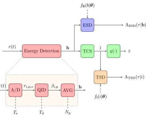
A/D Ts QID Td AVG Np Soft Decision Likelihood Calculator fB(b) Λ(τ |b) Hard Decision Decision Algorithm θd ˆ τ r(t) ri,p,s βi,p bi
Figure 3.1: Soft-decision and hard-decision energy detection system.
assumptions do not account for multipath fading or obstructed propagation, leading to inaccurate ranging in wireless environments.
A mathematical model is derived, which describes the range information by pro-viding range likelihood and range estimate for soft-decision and hard-decision lo-calization, respectively. The goal is to establish a range information model that accounts for the wireless environment and signal features to facilitate the design and analysis of optimal EDs. The key contributions are as follows:
• Derivation of a range information model for design and analysis of wideband ranging systems based on energy detection;
• Development of low-complexity ranging algorithms with optimal EDs for soft-decision and hard-soft-decision localization;
• Quantification of the benefits to location awareness provided by the proposed range information model in wireless environments.
Notation
For a random variable (RV) X, the x, fX(·), and FX(·) denote its realization,
dis-tribution function, and cumulative disdis-tribution function (CDF), respectively. Let X∼ N (µ, σ2) denote a Gaussian distributed RV with mean µ and variance σ2. Let
φ(·) and Φ(·) denote the PDF and CDF of a standard Gaussian RV, respectively. The symbol ⌊x⌋ denotes the largest integer less than or equal to x. Let 0 be the all-zero vector. The notation Ec denotes the complement of an event E.
3.1
Ranging System
This section describes the energy detection principle and formulates the statistical model for the energy samples at the ED’s output.
3.1.1
Energy Detection
Consider a ranging system composed of a transmitter at position pt that emits Np
copies of a signal s(t) with repetition period Tp, and a receiver at position pr. Several
techniques are available in the literature to estimate the repetition period of a signal when it is unknown, see e.g., [62]. The aim of the ranging system is to detect the signal s(t) and to estimate its TOA τ with respect to a reference time t0 from the
received signal based on Np observations each with duration Tobs. Range and TOA
are used interchangeably throughout this dissertation since the former is a bijective function of the latter. The reference time t0 can be the time at which the signal was
transmitted (e.g., TOA-based localization or radar systems) or be the time shared among several receivers (e.g., TDOA-based localization systems).
For ranging techniques based on energy detection, energy samples (namely energy bins) are collected, one for each dwell time Td. After band-pass filtering for noise
reduction (and clutter mitigation in case of SR), the received waveforms are non-coherently accumulated for soft-decision and hard-decision processing as illustrated in Figure 3.8. The received signal can be written as
r(t) = u(t) + n(t) (3.1)
where u(t) is the received probe signal after propagating through a wireless channel with impulse response h(t; ς) and n(t) is the thermal noise component. The received probe signal is a sequence of channel responses to the transmitted signal replicas, the first of which can be written as
u(t) = *
h(t; ς) s(t − ς) dς . (3.2)
The received signal is first sampled by an analog-to-digital (A/D) converter with sampling period Ts. At the sampling instant ti,p,s = i Td + p Tp + s Ts, with i =
0, 1, . . . , Nb− 1 and p = 0, 1, . . . , Np− 1, the sample of the received signal is given
by
where ui,p,s = u (ti,p,s) and ni,p,s= n (ti,p,s). After A/D conversion, waveform samples
are processed by a quadrature integrate and dump (QID) block that squares and integrates them over a dwell time Td to obtain Nb= ⌊Tobs/Td⌋ energy bins. The ith
energy bin corresponding to the pth observation is given by
βi,p = N$sb−1 s=0 r2(ti,p,s) = N$sb−1 s=0 (ui,p,s+ ni,p,s)2 (3.4)
where Nsb = ⌊Td/Ts⌋ is the number of signal samples per bin. The energy bins
obtained from each observation interval are processed by an averaging (AVG) block over the Np observations as
bi = 1 Np N$p−1 p=0 βi,p (3.5)
resulting in a vector of energy bins b = [ b0, b1, . . . , bNb−1]. The vector of energy bins
at the output of the ED is used as input for soft-decision or hard-decision processing. The detection of the signal s(t) and the estimation of its TOA τ are based on the energy bin vector b. Classical approaches follow the Bayesian hypothesis testing, involving the comparison of the energy bins with a threshold. Such a threshold is often chosen to achieve a constant false-alarm rate resulting in a certain misdetection rate.
Typically, ranging is based on hard-decision algorithms which provide the TOA estimate from the observed energy bins. If the distribution function of energy bins is known, then soft-decision algorithms can be conceived providing a posterior PDF of the TOA estimates. Models for soft-decision and hard-decision algorithms, which will be provided in Section 3.2, depend on the distribution of the energy samples given in the following.
3.1.2
Energy Samples
Each element bi of the vector b is an instantiation of the RV
Bi = N$sb−1 s=0 X(i,s)N p (3.6) where X(i,s)n = 1 n n−1 $ p=0 (Ui,p,s+ Ni,p,s)2 (3.7)
is the sample average, in p, of the energy bins. In particular, Ui,p,s and Ni,p,s are
independent random samples of the received probe signal and of the thermal noise, respectively. Note that Bi depends on the transmitted signal, thermal noise, true
TOA τ , wireless channel, and ED parameters. Let θ = [τ θh θd] where θhand θd are
the vectors of parameters representing the wireless channel and the ED, respectively. The normalized bin BiNp/σ2 conditioned on θ is distributed as a noncentral
chi-squared RV with NpNsb degrees of freedom, i.e.,
BiNp σ2
|θ
∼ χ2NpNsb(λi) (3.8)
where λi is the noncentrality parameter, which depends on θ, given by [44]
λi = N$p−1 p=0 N$sb−1 s=0 u2 i,p,s σ2 (3.9)
with ui,p,s denoting the instantiation of the RV Ui,p,s and σ2 denoting the variance
of the zero-mean thermal noise. Therefore,
fBi(b|θ) = Np 2σ2e −bNp+λiσ2σ2 2 + bNp λiσ2 ,NpNsb−2 4 INpNsb−2 2 -. λibNp σ2 / (3.10) FBi(b|θ) = e −λi2 +∞ $ r=0 (λi/2)r r! γ0NpNsb 2 + r, bNp 2σ2 1 Γ0NpNsb 2 + r 1 (3.11)
where Ia(·) is the modified Bessel function of the first kind with order a, γ(·, ·) denotes
the lower incomplete Gamma function, and Γ(·) denotes the Gamma function [63]. Remark 1. In practice, the noise variance can be estimated by observing the en-ergy bins in an absence of the transmitted signal and each λi depends on the wireless channel instantiation. Therefore, the derivation of the range estimation error dis-tribution requires averaging the conditional energy bin disdis-tribution over all possible wireless channel instantiations [37].
3.2
Range Information Model
This section offers the range information model by providing the range likelihood and the range estimate, as well as the range error.
3.2.1
Range Likelihood
The range likelihood function is determined from the observation bi in (3.5) and
the distribution of Bi for each energy bin, as shown in Figure 3.8. The RVs Bi’s are
independent and non-identically distributed with noncentrality parameter depending on θ. The range likelihood function for a given bins observation can be written as
Λ(ς|b) =
N&b−1
i=0
fBi(bi|ς, θh, θd) . (3.12)
Remark 2. The range likelihood function can be used for both soft-decision and hard-decision localization. For soft-decision localization, a localization algorithm can directly process the likelihood functions obtained from one or more receivers to deter-mine the position of a node. For hard-decision localization, a localization algorithm first obtains the TOA estimate by seeking a maximum of the range likelihood func-tion, and then processes such estimates from one or more receivers to determine the position of a node.
3.2.2
Range Estimate
A widely used approach for ranging is based on hard-decision algorithms that aim to determine the index ˆı of the first bin containing a portion of the transmitted signal energy. Therefore, the index ˆı can be thought as the instantiation of a discrete RV I taking value in the set B = {0, 1, . . . , Nb− 1}.
Let the TOA estimate ˆτ be the instantiation of the RV T with PDF fT(t|θ).
The RV T depends on I since ˆτ is chosen from the interval [ˆıTd, (ˆı + 1) Td).
Con-sider a bijective function ˆτ = g(ˆı), e.g., the TOA estimate is chosen to be the center of the interval as g(ˆı) = ˆıTd+ Td/2. Therefore, the distribution function fT(t|θ) of
the TOA estimate is determined by the distribution function fI(i|θ) of I. The fT(t|θ)
depends on θ since the RV I is a function of both the wireless channel and the ED. Various hard-decision algorithms have been proposed in the literature [29,37,64]. The most popular hard-decision algorithms are analyzed: threshold crossing search (TCS), maximum bin search (MBS), jump back and search forward (JBSF), and serial backward search (SBS) algorithms. These algorithms involve the comparison of each bin value with a corresponding threshold. Let the threshold crossing event be Cth = {∃i ∈ B : Bi > ξi} where ξi is the threshold for the bin Bi for i ∈ B. The
fI(i|θ) = 2 1 − FBi(ξi|θ) 3 & j∈Ii(i) FBj(ξj|θ) 2 1 −& n∈B FBn(ξn|θ) 3−1 (3.16) fI(i|θ) = 2 * +∞ 0 & j∈B\{i} FBj(b|θ) fBi(b|θ) db − * ξi 0 & j∈B\{i} FBj( ˘ξj(b)|θ) fBi(b|θ) db 3 ×21 −& n∈B FBn(ξn|θ) 3−1 (3.19) fI(i|θ) = 2 * +∞ 0 & j∈INw(i) FBj( ˘ξj(b)|θ) & j∈Ic Nw(i)\{i} FBj(b|θ) fBi(b|θ) db − * ξi 0 & j∈B\{i} FBj( ˘ξj(b)|θ) fBi(b|θ) db + $ m∈INw(i+Nw+1) * +∞ ξi & j∈Ii−m+Nw(i) FBj( ˘ξj(b)|θ) [FBi(b|θ) − FBi(ξi|θ)] × & j∈Ic i−m+Nw(i)\{i,m} FBj(b|θ) fBm(b|θ) db 32 1 −& n∈B FBn(ξn|θ) 3−1 (3.23) fI(i|θ) = 2 * +∞ 0 ˘ FBi−1( ˘ξi−1(b)|θ) & j∈B\{i−1,i} FBj(b|θ)fBi(b|θ) db − * ξi 0 & j∈B\{i} FBj( ˘ξj(b)|θ) fBi(b|θ) db + $ m∈INb−i−1(Nb) * +∞ ˇ ξm,i ˘ FBi−1( ˘ξi−1(b)|θ) & j∈Im−i(m) [FBj(b|θ) − FBj(ξj|θ)] × & j∈Ic m−i(m)\{i−1,m} FBj(b|θ) fBm(b|θ) db 32 1 −& n∈B FBn(ξn|θ) 3−1 (3.26) θ can be written as fI(i|θ) = P {Si∩ Cth|θ} /P {Cth|θ} (3.12)
where the event Si∩ Cth|θ = {i is selected, Cth|θ} and
P {Cth|θ} = 1 −
&
n∈B
FBn(ξn|θ) . (3.13)
Remark 3. In general, a different threshold ξi can be used for each bin index i when it is important to account for the variation among the energy samples.
Threshold Crossing Search
The TCS algorithm first searches for each bin value bi that crosses a threshold ξi for
all i ∈ B. The algorithm then selects, if Cth occurs, the bin index ˆı as the smallest i
for which bi > ξi. Mathematically,
ˆı|Cth
= min{i ∈ B|bi > ξi} . (3.14)
The PMF of the selected bin index I conditioned on Cth and θ is given by (3.12) with
event
Si∩ Cth|θ = {Bj ≤ ξj∀j ∈ Ii(i), Bi > ξi|θ} . (3.15)
The index set INw(m) is defined as INw(m) = B ∩ {m − Nw, m − Nw+ 1, . . . , m − 1}
and its complement over B as Ic
Nw(m) = B\INw(m). The set INw(m) is empty for
Nw ≤ 0. This leads to (3.16) shown at the top of the page. The choice of the
thresholds ξi’s affects the accuracy of the TOA estimation, as well as the detection
rate and the false-alarm rate.
Maximum Bin Search
The MBS algorithm first searches for the maximum value among all the bins with index i ∈ B. The algorithm then selects, if Cth occurs, the bin index ˆı as the i for
which bj ≤ bi for all j ̸= i. Mathematically,
ˆı|C= argmaxth
i∈B
bi. (3.17)
The PMF of the selected bin index I conditioned on Cth and θ is given by (3.12) with
event
Si∩ Cth|θ = {i is selected, i is the max, Cth|θ}
= {Bj ≤ Bi∀j ∈ B\{i}|θ} (3.18)
\{Bj ≤ ξj∀j ∈ B, Bj ≤ Bi∀j ∈ B\{i}|θ} .
This leads to (3.19) shown at the top of the page, with ˘ξj(b) = min{ξj, b}. Note
0 10 20 30 40 50 60 70 0 0.2 0.4 0.6 0.8 1 i fI (i |θ ) Simulation Model 0 10 20 30 40 50 60 70 0 0.2 0.4 0.6 0.8 1 i fI (i |θ ) Simulation Model 0 10 20 30 40 50 60 70 0 0.2 0.4 0.6 0.8 1 i fI (i |θ ) Simulation Model 0 10 20 30 40 50 60 70 0 0.2 0.4 0.6 0.8 1 i fI (i |θ ) Simulation Model
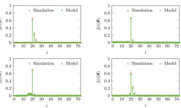
Figure 3.2: Example PMF of the selected bin index for the TCS (top left), MBS (top right), JBSF with Nw = 5 (bottom left), and SBS (bottom right) algorithms
with Td = 2 ns, Np = 128, and γ = −10 dB. The first bin containing the transmitted
signal has index i = 20.
(i.e., selecting the maximum bin even when none of the bins crosses its threshold). In such a case, (3.19) degenerates to the PMF of the selected bin index for MBS unconditioned on Cth, which is given by
fI(i|θ) = * +∞ 0 & j∈B\{i} FBj(b|θ) fBi(b|θ) db .
Jump Back and Search Forward
The JBSF algorithm first identifies the index m corresponding to the maximum bin value, jumps back to the bin with smallest index in INw(m), and searches forward
for each bin value bi that crosses a threshold ξi for all i ∈ INw(m). Here Nw denotes
the window length. For example, the window length Nw can be chosen according to
the channel delay spread and the transmitted signal. The algorithm then selects, if Cth occurs, the bin index ˆı as the smallest i for which bi > ξi or as m if none of them
crosses the threshold. Mathematically, ˆı|Cth
The PMF of the selected bin index I conditioned on Cth and θ is given by (3.12) with
events
Si∩ Cth|θ = Mi|θ ∪ Mci|θ (3.21a)
Mi|θ = {i is selected, i is the max, Cth|θ} (3.21b)
Mc
i|θ = {i is selected, i is not the max, Cth|θ} . (3.21c)
In particular, Mi|θ = {Bj ≤ ξj∀j ∈ INw(i), Bj ≤ Bi∀j ∈ B\{i}|θ} \{Bj ≤ ξj∀j ∈ B, Bj ≤ Bi∀j ∈ B\{i}|θ} (3.22a) Mc i|θ = 4 m∈INw(i+Nw+1) {Bj ≤ ξj∀j ∈ Ii−m+Nw(i), (3.22b) Bi > ξi, Bj ≤ Bm∀j ∈ B\{m}|θ} .
This leads to (3.23) shown at the top of previous page. The product is equal to 1 and the sum is equal to 0 if evaluated over an empty index set. Note that JBSF with Nw = 0 corresponds to MBS. In such a case, (3.23) degenerates to (3.19).
Serial Backward Search
The SBS algorithm first identifies the index m corresponding to the maximum bin value, and searches backward for each bin value bi that crosses a threshold ξi for
all i ∈ Im(m). The algorithm then selects, if Cth occurs, the bin index ˆı as the the
smallest i for which bj > ξj for all j ∈ Im−i(m) or as m if none of them crosses the
threshold. Mathematically,
ˆı|Cth
= min{{i ∈ Im(m)|bj > ξj∀j ∈ Im−i(m)} ∪ {m}} . (3.24)
The PMF of the selected bin index I conditioned on Cth and θ is given by (3.12) with
the events as in (3.21). In particular,
Mi|θ = {Bi−1≤ ξi−1 if i > 0, Bj ≤ Bi∀j ∈ B\{i}|θ}
\{Bj ≤ ξj∀j ∈ B, Bj ≤ Bi∀j ∈ B\{i}|θ} (3.25a) Mc i|θ = 4 m∈INb−i−1(Nb) {Bi−1≤ ξi−1 if i > 0, (3.25b) Bj > ξj∀j ∈ Im−i(m), Bj ≤ Bm∀j ∈ B\{m}|θ} .
This leads to (3.26) shown at the top of previous page, with ˘ FBk(·|θ) = ⎧ ⎨ ⎩ FBk(·|θ) for k ∈ B 1 for k /∈ B
and ˇξm,i = max{ξj∀j ∈ Im−i(m)}.
To illustrate how the hard-decision algorithms operate, consider a simple case of Nb = 8 bins (i.e., B = {0, 1, . . . , 7}) with a vector of bin instantiations and a vector
of thresholds given by
b= [0.8, 1.2, 1.3, 2.3, 2.5, 2.8, 2.4, 1.2] ξ = [1.3, 1.1, 0.9, 2.5, 1.4, 2.9, 1.9, 1.4] .
Note that the threshold crossing event is true (bins with index 1, 2, 4, and 6 cross the corresponding thresholds) and the algorithms select a bin index ˆı according to (3.14), (3.17), (3.20), and (3.24). In particular, ˆı = 1, 5, 2, and 4 for TCS, MBS, JBSF with Nw = 3, and SBS, respectively.
Remark 4. Recall that the PMFs fI(i|θ) for hard-decision algorithms derived above are conditioned on the threshold crossing event Cth and θ. Expressions for the joint PMF of I and Cthconditioned on θ can be obtained by ˇfI(i|θ) = fI(i|θ)
5
1 −6n∈BFBn(ξn|θ)
7
. The distribution fI(i|θ) of the selected bin index for numerous other hard-decision algorithms can be derived following a similar approach.
Figure 3.2 shows examples of PMF fI(i|θ) for the TCS, MBS, JBSF with Nw = 5,
and SBS algorithms with Td = 2ns, Np = 128, and γ = −10dB, according to the
IEEE 802.15.4a standard for indoor propagation [65]. It can be observed that the PMFs derived based on the proposed range information model are in agreement with those obtained through sample-level simulations (i.e., simulating the wireless channel and the ED operation). In particular, theory and simulations show the same bin index for which the PMF reaches its maximum value.
3.2.3
Range Error
The distribution of the TOA estimation error is now determined, which depends on the particular hard-decision algorithm. The TOA estimation error e(τ ) = ˆτ − τ is an instantiation of the RV E = T − τ, and thus
For a given τ , E belongs to a finite set Eτ = {T − τ s.t. T ∈ g(B)}, where g(B)
represents a finite set of TOA estimate. In the absence of a prior information on the true TOA, τ can be modeled as a uniform RV over the interval [0, Ta], where Ta is
the maximum possible TOA that depends on the wireless environment. This results in Eτ = [−Ta, Tobs] with, in general, 0 < Ta ≤ Tobs. When the wireless environment
is not known, Ta can be chosen as Ta = Tobs. Therefore,
fE(e|θd) = 1 Ta * Ta 0 fE(e|θd, τ ) dτ (3.27) where fE(e|θd, τ ) = ⎧ ⎨ ⎩ # # #d g−1d e(e+τ ) # # # fI(g−1(e + τ )|θd, τ ) for e ∈ Eτ 0 otherwise (3.28)
with fI(i|θd, τ ) = Eθh{fI(i|θ)}. For specific hard-decision algorithms, (3.28) can be
evaluated by substituting the PDF and CDF of Bi given respectively by (3.10) and
(3.11) into the specific conditional PMF fI(i|θ) derived in Section 3.2.2 and taking
the expectation over the vector of noncentrality parameters λ = [λ0, λ1, . . . , λNb−1].
Remark 5. The distribution of the TOA estimate requires both the evaluation of cumbersome expressions and the expectation over all the channel parameters. This calls for a tractable range information model.
3.3
Tractable Range Information Model
The design of soft-decision and hard-decision algorithms demands tractable expres-sions for the range information model, which can be obtained by simplifying fBj(b|θ)
and FBj(b|θ). First, recall that the chi-squared RV converges in distribution to a
Gaussian RV as the number of degrees of freedom increases. Therefore BiNp/σ2 in
(3.8) converges in distribution as BiNp σ2 d − → ˜Bi Np σ2 |θ ∼ N (NpNsb+ λi, 2(NpNsb+ 2λi)) (3.29) and consequently fBi(b|θ) ≃ Np/σ2 8 2(NpNsb+ 2λi) φ -bNp/σ2− NpNsb− λi 8 2(NpNsb+ 2λi) / (3.30) FBi(b|θ) ≃ Φ -bNp/σ2− NpNsb− λi 8 2(NpNsb+ 2λi) / . (3.31)
The above approximation depends on NpNsb and is accurate for Np 2 1 or Td 2
Ts. Note that the above distributions depend on the instantiation of the wireless
channel through θh in θ. However, the knowledge of the exact channel instantiation
is typically not available.
The range information model is further simplified by considering distributions that depend on channel statistics rather than channel instantiations, i.e., on θ = [τ θh θd] instead of θ, where θh represents the channel statistics. Recall that the
sample average X(i,s)n in (3.7) depends on [τ θh θd] through Ui,p,s and on θd through
Ni,p,s. Therefore we approximate X(i,s)n with Y(i,s)n in which Ui,p,s is replaced with a
deterministic quantity Ui,s that depends on θ as
Yn(i,s)= 1 n n−1 $ p=0 (Ui,s+ Ni,p,s)2 . (3.32)
A possible choice is Ui,s = E {Uν}1/ν, where E {Uν} is the νth order moment of U,
which is consistent in terms of the unit measure of Ui,s and Ni,p,s. Also, E {Uν}1/ν
is monotonically increasing in ν by Lyapunov’s inequality. The choice of Ui,s is
motivated by the following lemma.
Lemma 1. The sample average Z(i,s)n ! X(i,s)n − Y(i,s)n converges almost surely to 0 if and only if U2
i,s = E {U2}. Proof. First note that
Z(i,s,ν)n = 1 n n−1 $ p=0 5
U2i,p,s− Ui,s2 + 2Ni,p,s(Ui,p,s− Ui,s)7 .
Therefore, as n increases, Z(i,s)n converges to E {U2}−Ui,s2 almost surely by the strong
law of large numbers [66–68]. Thus, X(i,s)n converges almost surely to Y(i,s)n if and only
if U2 i,s = E {U2}. Lemma 1 suggests Bi ≃ 1 Np N$p−1 p=0 N$sb−1 s=0 +9 E:U2 i,p,s ; + Ni,p,s ,2 (3.33)
implying that the noncentrality parameter for BiNp/σ2 can be written as λi ≃ λi,
where λi = N$p−1 p=0 N$sb−1 s=0 E<U2i,p,s= σ2 . (3.34)
Remark 6. The dependence on wireless channel instantiations can be removed by substituting each noncentrality parameter λi, which depends on θ, with its expected value λi, which depends on θ, in all of the above distributions.
The impulse response of a wideband wireless channel at time t is commonly described by [69–73] h(t; ς) = L(t) $ l=1 αl(t) δ(ς − τl(t)) (3.35)
where L(t) is the number of multipath components, and αl(t) and τl(t) are the
amplitude gain and the arrival time of the lth path, respectively. The L(t), αl(t),
and τl(t) are considered time-invariant over an observation time.
For a resolvable multipath channel, i.e., the path interarrival time intrinsic to the wireless environment is larger than the temporal duration of the transmitted signal, E:U2i,p,s; in (3.34) can be written as
E:U2i,p,s; ≃ E< L $ l=1 α2ls2(ti,p,s− τl) = . (3.36)
Therefore, the calculation of λi requires the averaging with respect to the channel
nuisance parameters αl’s and τl’s in θh. The complexity of such calculation depends
on the joint distribution of L, αl’s, and τl’s. However, the resolution of the ED is
limited by the dwell time Td. Therefore, the statistics of the energy bins can be
determined by considering a tapped-delay-line model [7,73–76]. In particular, h(t; ς) can be replaced by ˘h(t; ς) =%Ll=1˘ α˘lδ(ς − ˘τl), where ˘L is a deterministic number of
path, ˘τl = τ + l∆ with ∆ deterministic, and ˘L∆ is the approximate dispersion of
the channel. For example, ∆ can be chosen as the dwell time, the inverse of the bandwidth, or the average interarrival time of the paths. This results in
E:U2i,p,s;≃ ˘ L $ l=1 E:α˘2l;s2(ti,p,s− ˘τl) . (3.37)
Substituting (3.37) in (3.34), the expected value of the noncentrality parameter for the ith bin becomes
λi = N$p−1 p=0 N$sb−1 s=0 ˘ L $ l=1 E {˘αl2} σ2 s 2(t i,p,s− ˘τl) . (3.38)
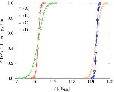
115 116 117 118 119 120 0.0 0.2 0.4 0.6 0.8 1.0 b [dBbin] C D F o f th e en er g y b in (A) (B) (C) (D)
Figure 3.3: Example CDF of the energy bin value for different values of Np and Td
with γ = −20 dB: (A) Np = 128, Td = 2ns; (B) Np = 16, Td = 2ns; (C) Np = 128,
Td = 4ns; (D) Np = 16, Td = 4ns. Simulation results are shown in symbols and
theoretical results according to (3.39) are shown in solid lines.
Using (3.38) instead of λi in all the above distributions, one can obtain the tractable
range information model that depends only on θ instead of θ. For instance, Bi can
be approximated by Bi with conditional CDF given by
FBi(b|θ) = Φ ⎛ ⎝bNp/σ2− NpNsb− λi 9 2(NpNsb+ 2λi) ⎞ ⎠ (3.39)
which is obtained from (3.31) by replacing λi with λi.
Figure 3.3 shows the CDF of the energy bin for different numbers of observations and dwell times with received signal-to-noise ratio (SNR) per pulse γ = −20dB according to the IEEE 802.15.4a standard for indoor residential LOS environments [65]. More details about the scenario will be provided in Section 3.3.2 where the case study is presented. It can be observed that the theoretical CDF of the bin value (3.39) accurately describes the empirical CDF obtained by sample-level simulations.
Using the results in this section, tractable expressions of the distribution of the TOA estimation error can be derived for hard-decision algorithms. In particular, substituting the PDF and CDF of Bi given respectively by (3.10) and (3.11) into the
conditional PMF fI(i|θ) in Section 3.2.2 for specific hard-decision algorithms, and
replacing each λi with λi, (3.28) is simplified into a tractable form.
Remark 7. The parameters λi’s depend on θh through ˘L, the statistics of ˘αl, and
∆. The λi’s depend on θd through Nsb and ti,p,s, which further depends on Td, Tp, and Ts.
3.3.1
Design of the Energy Detector
This section aims to present the design of energy detection algorithms based on the proposed range information model. Such a model enables us to determine ED param-eters (e.g., the choice of the thresholds, window length, and dwell time) according to different optimization criteria and constraints.
The design of ED commonly involves the probability of detection and that of false-alarm. The detection event occurs when, in a presence of the transmitted signal, the presence of the signal is correctly detected. The probability of such an event is given by Pd(θd) = $ i∈B ˇ fI(i|θd, λ ̸= 0) . (3.40)
The false-alarm event occurs when, in an absence of the transmitted signal, the presence of the signal is incorrectly detected due to noise. The probability of such an event is given by Pfa(θd) = $ i∈B ˇ fI(i|θd, λ = 0) . (3.41)
For a given minimum tolerable level of detection probability P⋆
d or maximum
toler-able level of false-alarm probability P⋆
fa, constraints on parameters value θd can be
obtained. For example, Pfa(θd) is non-increasing with the threshold ξ and therefore
a minimum value ξfa can be determined for a given Pfa⋆.
An important metric for ED design is the mean squared error (MSE) of the TOA estimate. When conditioned on the detection of the transmitted signal, the MSE of the TOA estimate is given by
ϱt(θd) =
* +∞
−∞
Recalling that the TOA estimation error belongs to a finite set Eτ, the MSE of the
TOA estimate for hard-decision algorithms can be written as
ϱt(θd) = 1 Tobs N$b−1 i=0 * Tobs 0 (g(i) − τ) 2f I(i|θd, τ )dτ . (3.43)
The design of an ED minimizing the MSE of the TOA estimate with a guaranteed minimum level of detection probability can be obtained by solving the following constrained optimization problem
ˆ
θd = argmin {θd: Pd(θd)≥Pd⋆}
ϱt(θd) . (3.44)
Instead of guaranteeing a minimum detection probability, the design of an ED can minimize the MSE of the TOA estimate with a guaranteed maximum level of false-alarm probability as ˆ θd = argmin {θd: Pfa(θd)≤P⋆ fa} ϱt(θd) . (3.45)
The design of an ED can also be formulated to maximize the detection probability Pd(θd) for a given maximum tolerable MSE ϱ⋆tof the TOA estimate, i.e.,
ˆ
θd = argmax {θd: ϱt(θd)≤ϱ⋆t}
Pd(θd) . (3.46)
Alternatively, the ED design can be based on a hybrid objective function where the optimization problem is formulated to minimize a metric involving the MSE of the TOA estimate and a penalty. The mathematical formulation of such an optimization problem can be written as
ˆ θd = argmin θd υt(θd) (3.47) where υt(θd) = ϱt(θd) Pd(θd) + ν(θd) 5 1 − Pd(θd) 7 (3.48) is the unconditional MSE of the TOA estimate and ν(θd) is a penalty in an
ab-sence of detection. The penalty ν(θd) can be chosen as a function of the detection
probability.
The above optimization problems are typical examples for the design of a ranging system. However, the proposed range information model is general and can be used to formulate other optimization problems that arise from energy detection applications.
3.3.2
Results
This section defines the performance metrics, describes the case study scenario, and presents performance results based on the developed theory and sample-level simu-lations.
Performance Metrics
Performance of the proposed range information model is evaluated in terms of the PMF accuracy, ranging accuracy, and localization accuracy defined as follows.
The following metrics will be used as a measure of the distance between the PMF fI(i|θ) of the selected bin obtained from the proposed range information model and
that obtained through sample-level simulations. Let p1, p2 be two possible PMFs
representing a RV taking values on a set X , e.g., one approximate and one exact. The Jensen–Shannon divergence (JSD) is defined as [77]
DJS{p1, p2} = 1 2 $ i∈X p1(i) log + 2 p1(i) p1(i) + p2(i) , + 1 2 $ i∈X p2(i) log + 2 p2(i) p1(i) + p2(i) , . (3.49)
Other important metrics are the root-mean-square error (RMSE), which is defined as DRMSE{p1, p2} = B 1 |X | $ i∈X |p1(i) − p2(i)|2 C1/2 (3.50)
and the maximum error, which is defined as DME{p1, p2} = max
i∈X {|p1(i) − p2(i)|} . (3.51)
The ranging accuracy is determined in terms of CDF of the TOA estimation error FE(e|θd) and in terms of RMSE of the TOA estimate ρt(θd) =
8
ϱt(θd). The
CDF FE(e|θd) and the RMSE ρt(θd) are obtained starting from (3.27) and (3.42),
respectively.
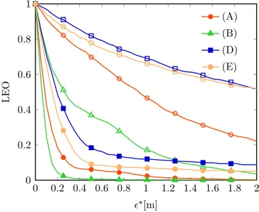
The localization accuracy is determined in terms of the localization error outage (LEO). The LEO is defined as the probability that the localization error is above a maximum tolerable value 2⋆, i.e.,
Po(θd) = Eθh : ((⋆ , +∞){2(p|θ)} ; (3.52)
where, for a set A, A{a} = ⎧ ⎨ ⎩ 1 for a ∈ A 0 otherwise
and 2(p|θ) = ∥ˆp(θ)−p∥ is the absolute value of the localization error, in which ˆp(θ) and p are the estimated position and the true position, respectively.
Wireless Scenario and Energy Detector Setting
Consider a network of anchors (nodes with known position) aiming to localize agents (nodes in unknown positions) in an indoor environment. Specifically, the network is composed of four anchors located at the corners of a square with side length equal to 10 m. Each anchor emits a sequence of UWB root-raised cosine pulses with pulse repetition period Tpr = 150 ns. The transmitted power spectral density is compliant
with the emission masks according to the following regulations: (a) Japan (Asia Pacific Telecommunity); (b) Europe (European Telecommunications Standards In-stitute) and Korea (Asia Pacific Telecommunity); (c) USA (Federal Communication Commission); and (d) China (Asia Pacific Telecommunity). The wireless medium follows the IEEE 802.15.4a channel model for UWB indoor residential LOS environ-ments [65] with Ta = 50 ns.
The received signal is processed based on energy detection with observation time Tobs = Tpr. In the case of hard-decision algorithms, ξi = ξ ∀i ∈ B is considered for
illustration. The value ξ is commonly chosen by accounting only for the randomness of the noise and discarding that of multipath propagation [78–80]. Alternatively, in [37], a simple criterion to determine a threshold is proposed based on the probability of early detection and on the knowledge of noise power. In contrast, the proposed range information model enables us to choose a threshold that accounts for the randomness of the wireless environments. The received SNR per pulse is γ = Ep/N0
where Ep is the energy of the received signal pulse and N0 is the one-sided power
spectral density (PSD) of the noise component. The noise has mean zero and variance σ2 = N0W where W is the bandwidth of the transmitted signal that depends on the
emission masks. Unless otherwise stated, the results in the following are provided for an emission mask as defined by the Federal Communication Commission with bandwidth W = 7.5 GHz, a number of bins Nb = 75, and a dwell time Td = 2 ns.
The threshold is chosen according to (3.44) as the ξ that minimizes the MSE of the TOA estimate with a guaranteed minimum level of detection probability P⋆
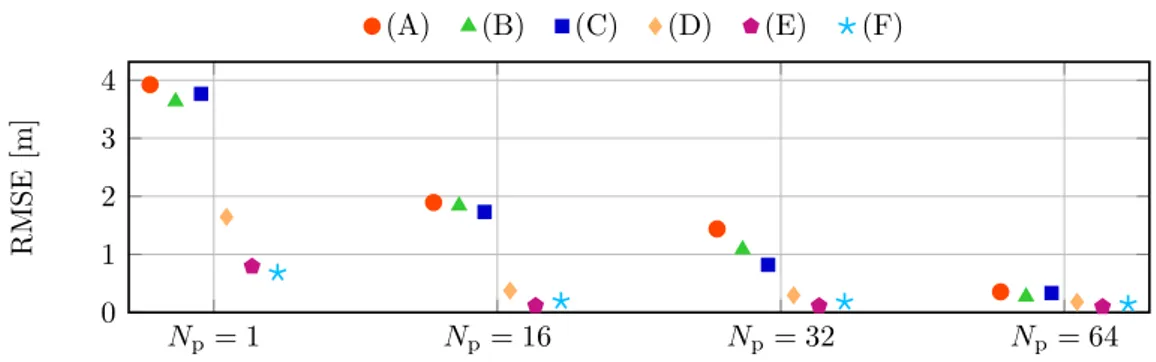
(A) (B) (C) (D) −150 −100 −50 0 50 100 150 0.0 0.2 0.4 0.6 0.8 1.0 eτ(τ ) [ns] CD F (a) TCS algorithm (A) (B) (C) (D) −150 −100 −50 0 50 100 150 0.0 0.2 0.4 0.6 0.8 1.0 eτ(τ ) [ns] CD F (b) MBS algorithm (A) (B) (C) (D) −150 −100 −50 0 50 100 150 0.0 0.2 0.4 0.6 0.8 1.0 eτ(τ ) [ns] CD F (c) JBSF algorithm (A) (B) (C) (D) −150 −100 −50 0 50 100 150 0.0 0.2 0.4 0.6 0.8 1.0 eτ(τ ) [ns] CD F (d) SBS algorithm
Figure 3.4: Example CDF of the TOA estimation error for the TCS, MBS, JBSF with Nw = 5, and SBS algorithms with different values of Np and γ: (A) Np = 128,
γ = −10 dB; (B) Np = 16, γ = −10 dB; (C) Np = 128, γ = −20 dB; and (D)
Np = 16, γ = −20 dB. Theoretical results are shown in solid lines and simulation