Aggregation of regional economic time series with different spatial correlation structures

! " # $ % & ' ( $ ) * +,- !& . /0 /

Aggregation of regional economic time series with different spatial

correlation structures

Giuseppe Arbia, University “G. d’Annunzio” of Chieti–Pescara (Italy) 1 Marco Bee, University of Trento (Italy)

Giuseppe Espa, University of Trento (Italy)

Abstract: In this paper we compare the relative efficiency of different

forecasting methods of space-time series when variables are spatially and temporally correlated. We consider the case of a space-time series aggregated into a single time series and the more general instance of a space-time series aggregated into a coarser spatial partition. We extend in various directions the outcomes found in the literature by including the consideration of larger datasets and the treatment of edge effects and of negative spatial correlation. The outcomes obtained provide operational suggestions on how to choose between alternative forecasting methods in empirical circumstances.

JEL classification: C15, C21, C43, C53

Keywords: Spatial correlation; Aggregation; Forecast efficiency; Space–time models; Edge effects; Negative spatial correlation.

1. Introduction

The problem of choosing the best forecasting strategy when dealing with disaggregated time series has a long tradition in econometrics. Giacomini and Granger (2004) (henceforth GG) faced this problem in the specific case of forecasting a national aggregate when disaggregated regional series are available and the individual regional series display spatial correlation. In the quoted paper the two strategies of aggregating the forecasts and forecasting the aggregate were compared in terms of asymptotic theoretical results and of small sample Monte Carlo simulations. The general conclusion of the paper was that “ignoring spatial dependence, and simply aggregating univariate forecasts for each region, leads to highly inaccurate forecasts“. In particular the authors showed that, if the variables observed at a regional level satisfy the ‘poolability’ condition (Kohn, 1982), there is a benefit in forecasting the aggregate variable directly. The authors themselves explicitly recognize the limits of their analysis by stating that: “the paper relied on many simplifications of the actual complexity of data measured in space and time and therefore it does not claim to be exhaustive”. In this paper we wish to extend their findings by removing some of the simplifications assumed in their study.

First of all GG restricted themselves to the case of positive spatial autocorrelation whereas here we consider the case in which the regional data can also display negative spatial correlation. Negative spatial correlation is less frequent than positive spatial correlation in economic analysis at coarse levels of spatial aggregation (like e.g. countries) where neighbours tend to display similar values, however they are very common in the case of spatial data observed at a fine level of disaggregation (like e.g. micro data on single plants or data aggregated at a communal level) where spatial distributions may be characterized by a chessboard structure due to local competition and

1_{Corresponding author. Department of the Business, Statistical, Technological and Environmental Sciences, University “G. d’Annunzio” of} Chieti-Pescara, Viale Pindaro, 42, 65127, Chieti-Pescara, Italy; phone and fax number: 0039 085 4537533; Email address: arbia@unich.it.

crowding–out phenomena (see Griffith, 2006; Griffith and Arbia, 2006). Therefore it deserves a special consideration in examining the problem of aggregated forecasts.

Secondly in their simulations GG considered only very small regular grids of data (the larger being constituted by a 4–by–4 grid of 16 spatial units) that could be dominated by border (or “edge”) effects (Griffith, 1983, 1985 and 1988). For this reason not only we consider, in our experiments, a larger number of sites (up to an 8–by–8 grid of 64 spatial units) which is closer to the typical dimension of a spatial series in regional economics, but we also include in the analysis a practical solution to the distortions due to borders when simulating bounded spatial series of data.

Thirdly GG considered the simpler case of aggregating regional series into a single national series. Here we wish to look at the more general case where data are available on a fine grid (e.g. counties within regions) and we have the problem of producing a forecast on a coarser grid (e.g. regions within a country). Our motivating example is based on the need, at a EU level, to produce forecasts for each member state (the NUTS1 level) and we avail time series of data at a regional level (the NUTS2 level); see Andreano and Savio (2005). So our approach is more general in that, whereas the final aim of GG was that of producing a univariate forecast, ours is to end up with a multivariate forecast.

The paper is organized as follows. In Section 2 we introduce the statistical framework to approach formally the problem and present a short account of the STAR (Space–Time AutoRegressive) class of models of random fields which will constitute the basis of our simulation study. In Section 3 we present the various alternative forecasting methods considered in the simulation. Section 4 is devoted to the Monte Carlo simulation design and to the interpretation of the results related to the univariate forecast (a space–time series collapsed into a single time series). In order to allow comparison of our results with those of GG we will consider the same forecasting strategies and the same combinations of the parameters’ values. However, our parametric set will be larger to allow negative spatial correlation and stronger spatial correlation to enter into discussion. In Section 5 we will extend our analysis to the case of multivariate forecasting (a space time series

of, say, n regions and T time periods aggregated into a coarser space–time series of k (k <n)

regions and T time periods). Finally Section 6 is devoted to some concluding remarks and general comments and to envisage possible future developments in the field.

2. Models of spatio–temporal dependence: the STAR class

The space–time autoregressive (STAR) class of models is a very flexible and popular framework considered in the literature by Cliff et al. (1975) and Pfeifer and Deutsch (1980); for a review see Upton and Fingleton (1985). In general terms the STAR models incorporate the spatio–temporal

Markov hypothesis by expressing the value of the variable x at location i and time t (say x ) _it

conditional upon the past history and the spatial context of the same variable. In the present paper we will consider, in particular, the following model STAR(1,1):

T t k i x x x _it k j jt ij it it , 1,..., ; 1,..., 1 1 1+ + = = =

∑

or, in matrix notation:

T t t t t t = x−1+ Wx−1+ε , =1,..., x φ ψ [2]

in which dependence is restricted to only the first lag both in time and space. Obviously there is no theoretical obstacle to extend the analysis to time lags higher then 1. In our case it is convenient to

restrict ourselves to isotropic models (Arbia, 2006) so that we can assume ψ_ij =ψw_ij, where ψ is

the single spatial autocorrelation parameter and w is the generic element of a weights’ matrix W _ij

such that w_ij =1 if location i and location j are neighbours according to a pre–defined criterion and

0 =

ij

w otherwise. If ψ =0, equation [1] reduces to the purely temporal autoregressive model of

order 1 (AR(1)). When ψ =0 and φ=1 it reduces to a simple random walk. Finally, when φ= 0 , it

reduces to the standard purely Simultaneous spatial Autoregressive model (SAR; Besag, 1974). As suggested by GG in their experiments, it is more sensible to employ a STAR rather than a simple

SAR model since the final aim is to evaluate the effects of spatial autocorrelation on forecasts

efficiency.

As it is known, when ψ =0 equation [1] represents a (weak–sense) time–stationary process if

the condition φ <1 holds. However, when ψ ≠0, the time–stationarity conditions are much more

complicated. We will simplify the discussion by restricting ourselves to the necessary, although not sufficient, stationarity condition:

φ+ψ w_ij

j=1 k

∑

Condition [3] is a natural way of introducing stationarity if we assume standardized weights

(so that 1 1 =

∑

w ) as we will do consistently in the rest of the paper. In this case the stationarity

condition reduces simply to φ+ψ < 1 .

Model [2] can be seen as a particular case of a VAR(1) model (see Lütkepohl, 1993, p. 167–

178) and can be expressed as xt = Axt−₁+εt, 1,...,t= T with the restriction imposed on the matrix A

of the autoregressive parameters that A=

(

)

straightforward: the global amount of autocorrelation that is present in a system of equations is limited by spatial proximity.

3. Definition of the forecasting strategies and of the various simulation scenarios

In this paper we are interested in identifying the best forecasting strategy in cases where we have data on a n–dimensional time series referred to a certain partition of the space and we need to

produce a forecast for a k–dimensional (k <n) time series referred to k fewer and larger partitions

of the same space. For instance we have data on sub–regional product and we wish to forecast the temporal evolution of regional GDP. In the present and in the following sections, however, we will

start considering the simpler case in which k =1. This is the case analysed by GG and we will

therefore be able to compare our results with those obtained therein. In Section 5 we will extend our

attention to the more general case where k >1.

Let us start assuming that the (single) aggregate time series S_t

( )

aggregation of k disaggregated series such that

( )

1 k t t it i S y x = = =

∑

{ }

(

)

• Scenario f1. A forecast for y is directly obtained by adapting a univariate time series model _t

to the aggregate series

{ }

t t

y ₌₁. In practice the forecast is thus obtained by making use of only

the aggregate information. This scenario corresponds to the strategy of forecasting the

aggregate.

• Scenario f2. In this case a forecast for y is obtained by forecasting individually each time _t

series x _it

(

)

to the strategy of aggregating the forecast.

• Scenario f3. A vector time–series model (VAR) is fitted to the individual series neglecting any

spatial correlation effects, and a forecast vector is obtained. The forecast for y is then _t

obtained by aggregating the individual forecasts for each x . _it

• Scenario f4. A forecast for each x , _it i=1,...,k, is obtained by employing a STAR model, thus

including explicit consideration of spatial correlation effects, and the forecast for y is then _t

obtained by aggregating the individual forecasts for each x _it

Both scenarios f1 and f2 do not consider the specificity of the space–time components, while in both f3 and f4 we exploit all the information available not only on the univariate series, but also on their dependence structure. In particular, scenario f4 takes spatial dependence explicitly into account in the forecasting.

In the simulation experiments that will be presented in Sections 4 and 5, we will compare the

accuracy of the various forecasting procedures in terms of the one–step forecast of the value of y _t

conditional on the information available at time t−1 (say y_t−1

( )

of this forecast we will use the classical forecasting MSE definition provided by:

MSE y

(

( )

)

(

( )

)

GG derived a series of large–sample analytical results both in the case of known parameters and in the case of parameters that are estimated on the basis of empirical data. Such results are the natural extension of those derived by Lütkepohl (1987) for purely time series to series that display a certain degree of spatial autocorrelation. The main results are that, when the parameters are

assumed to be known and the poolability condition2 is not satisfied, strategy f3 dominates both f1

and f2 (f3_ff2 and f3_ff1) in terms of MSE and is equivalent to strategy f4. Conversely, when the

poolability condition holds, f3 is equivalent to the f1 strategy and the previous ranking among forecasting methods is not valid any more. These results have a limited practical interest in that, in empirical circumstances, the model’s parameters have to be estimated from data and so they cannot be considered as known prior to the estimation procedure. In the latter setup the f3 Scenario loses its optimality characteristics and the ranking among the various forecasting strategies will depend on the specific data generating process that can be assumed. When the generating mechanism is a

STAR(1,1) model, GG proved that, asymptotically in T:

2_{In the specific modelling framework that will be employed in the present study (that is a}

STAR(1,1) model) the poolability condition implies that

wij=ν i=1

k

∑ , ∀i which is rarely satisfied in practical circumstances. Among the regular spatial schemes that we use in the simulation experiments only the 2×2 scheme has associated a W matrix satisfying the poolability condition if we consider the rook’s case definition of neighbours (Cliff and Ord, 1981).

( )

(

)

with T the sample size and yˆ_t−1

( )

ˆ

θ_T to the true parameter vector θ₀ in the linear predictor of y (say _t y_t−1

( )

From equation [4] it is evident that the component of MSE depending on the estimation error

(1 2k2

Tσ ) increases proportionally to the square of the number of regions (

2

k ) whereas the

component that is present also in the case of known parameters (σ2k) increases with k. This

explains intuitively why in the case of estimated parameters, scenario f3 does not dominate the others any more. In fact, there is a trade–off between a forecast based on disaggregated series where we have no loss of information (but a very high number of spatial observation), and the loss of efficiency deriving from an uncontrolled value of k. Having said that, the only possible ranking

between the various scenarios is that both f4 and f1 dominate f3 (f4_ff3 and f1_ff3), but no ranking

is possible between f3 and f4 criteria. Notice that, however, the dominance of f1 on f3 holds true only when the poolability condition is satisfied and depends on the number of spatial observations: the greater is this number, the greater is the gain in efficiency.

When the poolability condition holds, it is possible to derive the explicit expression of the

process generating the aggregate series y also for a finite sample size as we will prove in the _t

following proposition.

Proposition 1. Under the poolability condition, the process of the aggregate

1 k t it i S x = =

∑

with parameter φ ψν+ , where

1 k ij i w ν = =

∑

Proof. If the poolability condition holds, the matrix W has equal column sums 1 k ij i w ν = =

∑

matrix notation, the model is given by:

[

]

t = φ k +ψ t− + t

x I W x ε . [5]

3_{For example, in the case where =4}

k the W matrix is given by

0 0.5 0.5 0 0.5 0 0 0.5 0.5 0 0 0.5 0 0.5 0.5 0 ⎛ ⎞ ⎜ ⎟ ⎜ ⎟ =_{⎜ ⎟} ⎜ ⎟ ⎝ ⎠ W

In this case the poolability condition [4] holds with ν =1 and the equations of the model are:

1, 1, 1 2, 1 3, 1 1, 2, 2, 1 1, 1 4, 1 2, 3, 3, 1 1, 1 4, 1 3, 4, 4, 1 2, 1 3, 1 4, 2 2 2 2 2 2 2 2 t t t t t t t t t t t t t t t t t t t t x x x x x x x x x x x x x x x x ψ ψ φ ε ψ ψ φ ε ψ ψ φ ε ψ ψ φ ε − − − − − − − − − − − − = + + + = + + + = + + + = + + +

Summing up the four equations we get

( ) ( ) ( ) ( ) ( ) ( ) 1 1, 1 2, 1 3, 1 4, 1 1 , t t t t t t t t t S S x x x x S S S φ ψ ψ ψ ψ ε φ ψ ε − − − − − − = + + + + + = = + + x x x

Let

( )

∑

x . Summing up Equations [5] for all regions we obtain:

( )

( )

( )

( )

( )

( )

( )

∑

∑

∑∑

∑

∑ ∑

which is an AR(1) process with parameter φ ψν+ . Q.E.D. ■

When the poolability condition does not hold, it is easy to verify that the process of the

aggregate S_t

( )

( )

( )

( )

∑

=

∑

other, the process can be approximated by an AR(1) process.

All the previous results are based on quite restrictive assumptions of limited practical relevance. In order to obtain a more satisfactory ranking among the different prediction methods to assist the choice in practical circumstances, GG considered a set of small–sample Monte Carlo experiments whose results will be summarized in the next section. In the next section we will also extend their results to a wider variety of simulation cases.

4. Univariate aggregate forecasting from a STAR model 4.1 Simulation design

The Monte Carlo experiments reported in this section are based on various realizations of the

STAR(1,1) model presented in Equation [2]. It has been shown in the preceding Section 3 that the MSE is related both to the time horizon and to the number of regions. For this reason, in addition to

the cases of k=4,6,9,16 regions considered by GG, we also include the cases of a larger number

of regions with k=25,36, 49,64. In this way we can monitor more closely the interaction between

the spatial dimension and the efficiency of the various forecasting procedures. There is also a second important reason why we will consider a larger number of regions in our simulations, and it is connected with the problem of “edge effects” (see Griffith, 1988). Edge effects arise from the different behavior of border regions with respect to the inner regions in terms of the elements of the

W matrix. Such a problem has been addressed in the paper by GG, but no solution has been

proposed to overcome it. Intuitively, the distortion connected with edge effects will tend to disappear as the number of regions increases, in that the proportion of bordering regions with respect to the total number of regions becomes more and more negligible. This provides a further motivation towards large spatial schemes in the present context. In order to quantify the impact of edge effects, we can consider an indicator defined as

(

) (

)

EE= +

Such an index represents the proportion of information lost by ignoring the edge effects

divided by the total information available. When the system is a

(

)

k

EE =1 ; if the system is rectangular Cartesian lattice with dimensions

(

)

c c r

EE =( + ) 2 .

Just to give a flavor of the importance of the edge effects, Figure 1 reports the plot of the EE

index with respect to the number of regions. The values of EE range from 0.5 when k=4 to 0.125

when k =64, and show that the impact of edge effects becomes significantly less relevant when k

increases. In our simulations we have exploited the usual solution to edge effects that consists in the strategy of simulating a larger spatial scheme with respect to the target dimension of cells, to discard a buffer zone represented by the bordering cells of the scheme and to concentrate the analysis on the remaining cells (see Griffith, 1988; Ripley, 1981).

0 0,1 0,2 0,3 0,4 0,5 0,6 0 50 100 150 Number of regions EE

Figure 1: Edge Effect index (EE) plotted against the number of regions.

An important issue in setting the simulation experiments concerns the choice of the numerical

values of the parameters φ and ψ of the STAR(1,1) model considered in Equation [1], connected

respectively with temporal and spatial dependence. We decided to expand in two directions the range of values considered by GG.

First of all, in addition to the values corresponding to a low (ψ = 0.1) and to an intermediate

level ( ψ = 0.45 ) of spatial dependence, we also considered a high value ( ψ = 0.8 ) describing the

case of strong spatial dependence that was not considered in GG. As already discussed in the

preceding section, for the process to be stationary, the condition φ ψ+ < must be satisfied, thus, in 1

these instances, we could only consider two parameter configurations, namely the pair

(

) (

)

(

) (

)

Secondly, for the sake of completeness we also introduced the case of negative spatial correlation that (as argued in the introductory section) can represent an empirically relevant case in many regional economic applications. The numerical values of the parameters considered in the simulation are thus the following:

(

) (

)

(

) (

)

(

) (

)

(

) (

)

(

) (

)

(

) (

)

In the simulations we employ the four forecasting scenarios discussed in the previous Section

2. More in details, as for Scenario f1 we aggregate, at each time t (t= K ), the observed data 1, ,T

1t kt

x ,_K, x of the k regions. In this way we obtain a single aggregated time series. We then fit an

ARMA(p,q) model to S and compute the forecasts accordingly. We fit all ARMA(p,q) processes _t

with p=0 1, ,_{K , and} ,4 q=0 1, ,_{K , and such that 0},4 < + < , and choose the model that p q 5

achieves the smallest BIC value4.

Concerning Scenario f2 we start fitting an ARMA model to each individual regional time series. Again, the orders of the i–th ARMA model are determined using the BIC criterion. We then

compute the k univariate forecasts, say ˆx_{i ,T h+} , based on the estimated ARMA model. Finally, we

aggregate the ˆx_{i ,T h+} to obtain the aggregated forecasts

1 k T h i ,T h i ˆ _ˆ S ₊ x ₊ = =

∑

In the third Scenario (f3) we fit a VAR(1) model to the k–variate time series x_t, obtaining the

maximum likelihood estimate ˆA, and compute the one–step forecast _{ˆt 1} ˆ _t

+ =

x Ax ; both estimation

and prediction are based on standard VAR methodology (Lütkepohl, 1993).

Finally for Scenario f4 a STAR(1,1) process can also be written as a VAR(1) as in Scenario f3,

but now with the restrictions A=φW +ψI_k.The forecasts are then computed as in the f3 scenario.

In addition to the scenarios f1–f4 we introduced a modification of scenario f3 in order to take into account the possibility of having a large number of elements of A that are not significantly different from zero. This issue can be particularly relevant, in the sense that the number of elements

that are non significantly different from zero can be very large for small values of φ and/or of ψ .

Thus Scenario f3new consists of fitting a VAR(1) model to the k–variate time series, dropping the non–significant coefficients, re–estimating the model constraining to zero the non–significant coefficients and computing the forecast accordingly.

In all five cases the parameters are estimated via Maximum Likelihood. All the models considered here satisfy the regularity conditions required for the optimality properties of the estimators.

Having described the setup of the simulation and before presenting the results obtained, let us now examine into a greater detail the various computational steps involved by the experiments.

The first step consists of simulating 300 time observations from a STAR(1,1) process laid on a

regular square lattice grid. We treat the first T =200 observations as in–sample observations and the

last 100 observations as out–of–sample observations to be used to evaluate the forecast accuracy.

We start simulating k* regions arranged on a k∗ −by− k∗ regular square lattice grid. We then

discard 4

(

)

concentrate on the remaining = ∗−4

(

)

k k

k cells.

In a second step, we use the in–sample data to estimate the parameters of the different models corresponding to all the forecasting scenarios.

4_{The Bayesian Information Criterion (BIC) used in scenarios f1 and f2 was introduced by Schwarz (1978) to choose the “best member” of a set of} models. Here, the best model is meant to be the one that maximizes the posterior probability of the model given the data. It can be shown that, asymptotically, it is the one which minimizes the quantity: BIC= − 2(log maximized likelihood)+(number of parameters)log(T). The rule is similar to the Akaike Information Criterion, but the penalty for introducing new parameters is greater in BIC. As a consequence, simpler models are more likely to be selected when using BIC than when using AIC.

In a third step, for each forecasting scenario, we compute the Mean Squared Error as

(

)

=

∑

sample observations x_{i T h, +} .

Finally we repeat B times (B=500) the three preceding steps and compute the average MSE

over all the replications.

From a computational point of view, simulating the STAR(1,1) process is not particularly heavy. On the other hand, estimation is rather cumbersome. Scenarios f1 and f2 require indeed the computation of Maximum Likelihood estimates of ARMA models. In particular, scenario f2 requires

the estimation of k×14 ARMA models for each replication (14 being the number of different ARMA

models estimated under the condition p=0 1, ,_{K , 0 1},4 q= , ,_{K and 0},4 < + < ). Since the p q 5

ARMA likelihood has to be maximized numerically, the computational burden is relevant. As for

scenarios f3, f3new and f4, estimators can be obtained in a closed form, but the size of the matrices involved becomes extremely large as k increases (due to the presence of Kronecker products in the formulas of the restricted estimators of the VAR parameters). As a consequence the computing time is not negligible in these cases as well. Notwithstanding the enormous capabilities of the computers nowadays, the computing time has been demanding. A Pentium 4, 3.00 GHz, 2Gb RAM computer took a very long time in order to produce the required output.

4.2. Analysis of the simulation results

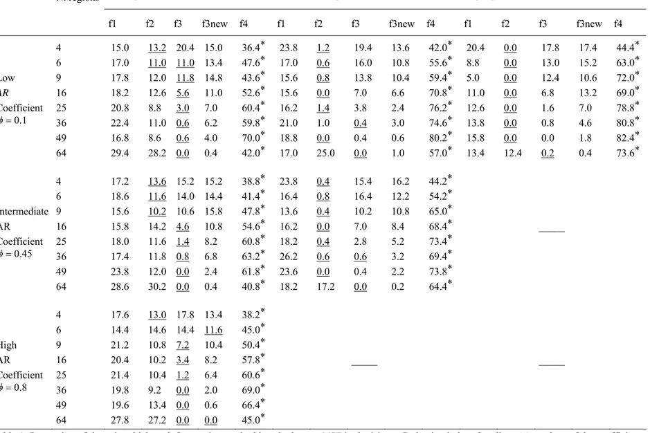
We will start by considering the average MSE achieved by the five forecasting scenarios for all parameters’ combination. The results are reported in Figure 2 and in Tables 1 and 2 where the MSE is expressed as a function of the spatial dimension of the grid considered. In particular, in order to provide a ranking among the various forecasting methods in terms of their accuracy, Tables 1 and 2 display the percentage of times in which each method performs the best.

The main conclusions that we can draw from this comparison are the following:

(1) The predictions obtained with the STAR model (Scenario f4) are always the most accurate, for all configurations of temporal and spatial dependence;

(2) The worst performing scenarios are those based on the univariate approach (f2) and on the unrestricted VAR (f3). There are two more conclusions connected with this point. First, when

the spatial parameter ψ is large in absolute value, the worst performing scenario tends to be

the univariate approach, whereas in presence of weak spatial dependence the worst results are obtained with the unrestricted VAR. Second, in all parameter configurations, as the number of cells k increases, the unrestricted VAR shows the worst performance.

(3) In all parameter configurations and in all scenarios, the average MSE increases with the spatial dimension. This result is consistent with the findings of GG. There is, however, a significant exception for the univariate scenario f2. In this case, when the number of regions increases from 49 to 64, for most parameter configurations the MSE decreases. In the other cases it increases at a slower rate. In particular, we observe a decrease when the spatial

dependence parameter ψ is large in absolute value, and a slower increase when ψ is small in

absolute value.

(4) The results of the negative dependence cases are essentially (i.e., apart from Monte Carlo variability) identical to the corresponding positive dependence cases when the parameters are equal in absolute value. In other words, it only matters the absolute value of the temporal and

4 6 9 16 25 36 49 64 10 20 30 40 50 60 70 80 90 100 Number of regions A v erage M S E φ = 0.1, ψ = 0.1 Aggregate Univariate VAR RVAR STAR 4 6 9 16 25 36 49 64 10 20 30 40 50 60 70 80 90 100 Number of regions A v e rage M S E φ = 0.1, ψ = 0.45 Aggregate Univariate VAR RVAR STAR 4 6 9 16 25 36 49 64 10 20 30 40 50 60 70 80 90 100 Number of regions A v er ag e M S E φ = 0.45, ψ = 0.1 Aggregate Univariate VAR RVAR STAR 4 6 9 16 25 36 49 64 10 20 30 40 50 60 70 80 90 100 110 Number of regions A v erag e M S E φ = 0.45, ψ = 0.45 Aggregate Univariate VAR RVAR STAR 4 6 9 16 25 36 49 64 20 40 60 80 100 120 Number of regions Ave ra g e M S E φ = 0.1, ψ = 0.8 Aggregate Univariate VAR RVAR STAR 4 6 9 16 25 36 49 64 20 40 60 80 100 120 140 160 180 Number of regions A v e rag e M S E φ = 0.8, ψ = 0.1 Aggregate Univariate VAR RVAR STAR 4 6 9 16 25 36 49 64 20 40 60 80 100 120 Number of regions A v erage M S E φ = -0.1, ψ = -0.8 Aggregate Univariate VAR RVAR STAR 4 6 9 16 25 36 49 64 20 40 60 80 100 120 140 160 180 Number of regions A v e rag e M S E φ = -0.8, ψ = -0.1 Aggregate Univariate VAR RVAR STAR 4 6 9 16 25 36 49 64 10 20 30 40 50 60 70 80 90 100 110 Number of regions A v e rage M S E φ = -0.45, ψ = -0.45 Aggregate Univariate VAR RVAR STAR

Figure 2: Average MSE over the B= 300 Monte Carlo replications for the various combinations of the parameters φandψ , plotted as a function of the number of regions used in

N. regions Low spatial coefficient ψ =0.1 Intermediate spatial coefficient ψ =0.45 High spatial coefficient ψ =0.8

f1 f2 f3 f3new f4 f1 f2 f3 f3new f4 f1 f2 f3 f3new f4

4 15.0 13.2 20.4 15.0 36.4* 23.8 1.2 19.4 13.6 42.0* 20.4 0.0 17.8 17.4 44.4* 6 17.0 11.0 11.0 13.4 47.6* 17.0 0.6 16.0 10.8 55.6* 8.8 0.0 13.0 15.2 63.0* Low 9 17.8 12.0 11.8 14.8 43.6* 15.6 0.8 13.8 10.4 59.4* 5.0 0.0 12.4 10.6 72.0* AR 16 18.2 12.6 5.6 11.0 52.6* 15.6 0.0 7.0 6.6 70.8* 11.0 0.0 6.8 13.2 69.0* Coefficient 25 20.8 8.8 3.0 7.0 60.4* 16.2 1.4 3.8 2.4 76.2* 12.6 0.0 1.6 7.0 78.8* 0.1 φ= _{36 22.4 11.0 0.6 6.2 59.8* 21.0 1.0 0.4 3.0 74.6* 13.8 0.0 0.8 4.6 80.8*} 49 16.8 8.6 0.6 4.0 70.0* 18.8 0.0 0.4 0.6 80.2* 15.8 0.0 0.0 1.8 82.4* 64 29.4 28.2 0.0 0.4 42.0* 17.0 25.0 0.0 1.0 57.0* 13.4 12.4 0.2 0.4 73.6* 4 17.2 13.6 15.2 15.2 38.8* 23.8 0.4 15.4 16.2 44.2* 6 18.6 11.6 14.0 14.4 41.4* 16.4 0.8 16.4 12.2 54.2* Intermediate 9 15.6 10.2 10.6 15.8 47.8* 13.6 0.4 10.2 10.8 65.0* AR 16 15.8 14.2 4.6 10.8 54.6* 16.2 0.0 7.0 8.4 68.4* _____ Coefficient 25 18.0 11.6 1.4 8.2 60.8* 18.2 0.4 2.8 5.2 73.4* 0.45 φ= _{36 17.4 11.8 0.8 6.8 63.2* 26.2 0.6 0.6 3.2 69.4*} 49 23.8 12.0 0.0 2.4 61.8* 23.6 0.0 0.4 2.2 73.8* 64 28.6 30.2 0.0 0.4 40.8* 18.2 17.2 0.0 0.2 64.4* 4 17.6 13.0 17.8 13.4 38.2* 6 14.4 14.6 14.4 11.6 45.0* High 9 21.2 10.8 7.2 10.4 50.4* AR 16 20.4 10.2 3.4 8.2 57.8* _____ _____ Coefficient 25 21.4 10.4 1.2 6.4 60.6* 0.8 φ= _{36 19.8 9.2 0.0 2.0 69.0*} 49 19.6 13.4 0.0 0.6 66.4* 64 27.8 27.2 0.0 0.0 45.0*

Table 1: Proportion of times in which each forecasting method has the lowest MSE in the Monte Carlo simulation, for all positive values of the coefficients φ and ψ. An asterisk

N. regions High negative spatial coefficient ψ = −0.8 f1 f2 f3 f3new f4 4 24.4 0.0 15.8 14.8 45.0* 6 11.0 0.0 14.0 13.4 61.6* Low 9 3.4 0.0 9.2 12.2 75.2* Negative 16 13.8 0.0 5.4 10.6 70.2* AR 25 12.8 0.0 2.0 8.2 77.0* Coefficient 36 15.0 0.0 1.6 4.2 79.2* 49 18.6 0.0 0.4 2.4 78.6* 64 14.2 15.2 0.0 0.2 70.4*

N. regions Intermediate negative spatial coefficient ψ = −0.45

f1 f2 f3 f3new f4 4 23.4 1.6 15.0 15.4 44.6* 6 15.8 0.8 12.6 13.6 57.2* Intermediate 9 12.6 0.6 8.8 10.4 67.6* Negative 16 16.2 0.0 6.6 6.6 70.6* AR 25 18.4 0.4 1.8 5.8 73.6* Coefficient 36 23.4 0.6 0.8 2.8 72.4* 49 20.0 0.4 0.2 1.8 77.6* 64 15.8 17.8 0.0 0.6 65.8*

N. regions Low negative spatial coefficient ψ = −0.1

f1 f2 f3 f3new f4 4 20.4 10.8 15.6 12.4 40.8* 6 15.6 9.4 11.0 14.4 49.6* High 9 16.0 10.2 9.6 13.0 51.2* Negative 16 15.8 11.4 4.0 8.0 60.8* AR 25 19.4 11.0 1.0 7.4 61.2* Coefficient 36 16.2 11.6 0.2 3.0 69.0* 49 17.2 9.8 0.0 1.0 72.0* 64 31.0 25.4 0.0 0.2 43.4*

Table 2: Proportion of times in which each forecasting method has the lowest MSE in the Monte Carlo simulation, for negative values of the coefficients φ and ψ. An asterisk indicates that the forecasting method in the corresponding column is the best the highest number of times, while the underline denotes the worst performing method.

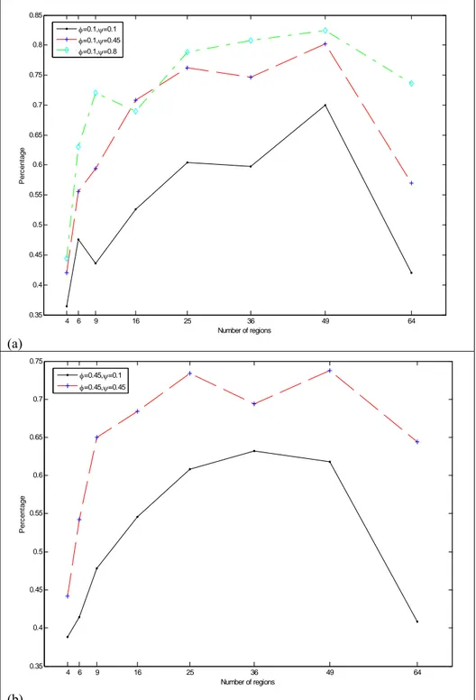
(5) The percentage of cases in which scenario f4 performs the best increases as the spatial dependence parameter gets larger. In other words, a correct specification of the model seems to be more important in presence of strong spatial dependence. This last conclusion emerges more clearly by inspecting Figure 3, which displays the percentage of times in which Scenario f4 has the lowest MSE plotted as a function of k for different parameter configurations. The

idea is to use this graph to compare this percentage when ψ increases, by holding constant

(

) (

)

(

) (

)

(

) (

)

(

) (

)

larger values of the spatial parameter. For instance when k=64 and φ =0.1, f4 approach

outperforms the other forecasting methods in the 42% of the cases examined, while the

percentage raises up to 73.6% when ψ =0.8.

(6) The percentage of cases where f4 outperforms the other methods is not a monotonic function of the spatial dimension. It increases with the number of regions up to a dimension of k = 49 and then it decreases.

4 6 9 16 25 36 49 64 0.35 0.4 0.45 0.5 0.55 0.6 0.65 0.7 0.75 0.8 0.85 Number of regions P e rc ent age φ=0.1,ψ=0.1 φ=0.1,ψ=0.45 φ=0.1,ψ=0.8 (a) 4 6 9 16 25 36 49 64 0.35 0.4 0.45 0.5 0.55 0.6 0.65 0.7 0.75 Number of regions P e rc ent age φ=0.45,ψ=0.1 φ=0.45,ψ=0.45 (b)

Figure 3: Percentage of times that scenario f4 has the lowest MSE, as a function of the number of regions, for (a) φ=0.1

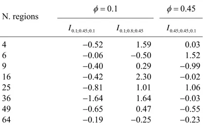
In order to measure the improvement in efficiency obtained with model f4 when the spatial parameter increases, we consider the ratio:

1 2 1 2 2 , , , , , MSE MSE I MSE φ ψ φ ψ φ ψ ψ φ ψ − = , where

MSEφ,ψi (i=1,2) is the average MSE, computed over all the iterations, obtained from the

simulation experiment with parameters φ and ψ . Thus, the index measures the rate of variation of

the MSE, for any fixed values of φ and k, when ψ increases. In particular, negative values of the

index correspond to efficiency gains, whereas positive values correspond to efficiency losses.

The results reported in Table 3 display a clear trend from weak (ψ =0.1) to intermediate

(ψ =0.45) spatial dependence: for all values of k the MSE decreases, and the rate of decrease is

particularly pronounced for k=25, 36 and 49. The results are less conclusive in the remaining two

setups (third and fourth column of the table), but it is worth noting that, when k =64, going from a

smaller to a larger value of ψ always provides more accurate forecasts.

1 . 0 = φ φ=0.45 N. regions I_0.1;0.45;0.1 I_0.1;0.8;0.45 I_{0.45;0.45;0.1} 4 −0.52 1.59 0.03 6 −0.06 −0.50 1.52 9 −0.40 0.29 −0.99 16 −0.42 2.30 −0.02 25 −0.81 1.01 1.06 36 −1.64 1.64 −0.03 49 −0.65 0.47 −0.55 64 −0.19 −0.25 −0.23

Table 3: Values of the index Iφ,ψ₁,ψ₂ for the numbers of regions considered in the experiment.

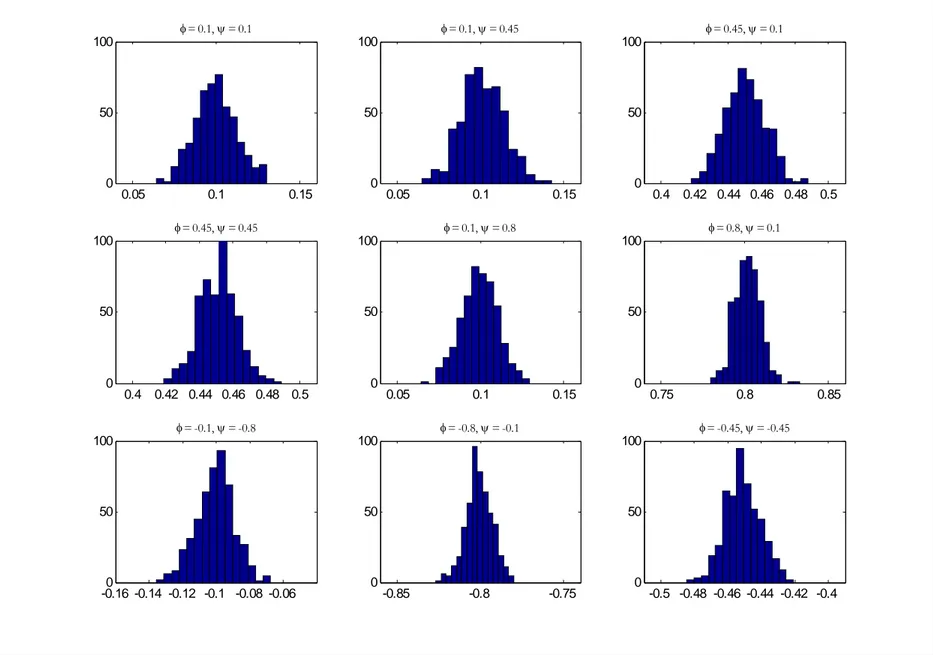
Figures 4 and 5 respectively show the estimates of φ and ψ obtained from the STAR(1,1)

model with k =64. The visual inspection suggests that the estimators are consistent and

asymptotically normal, as expected from the maximum likelihood theory.

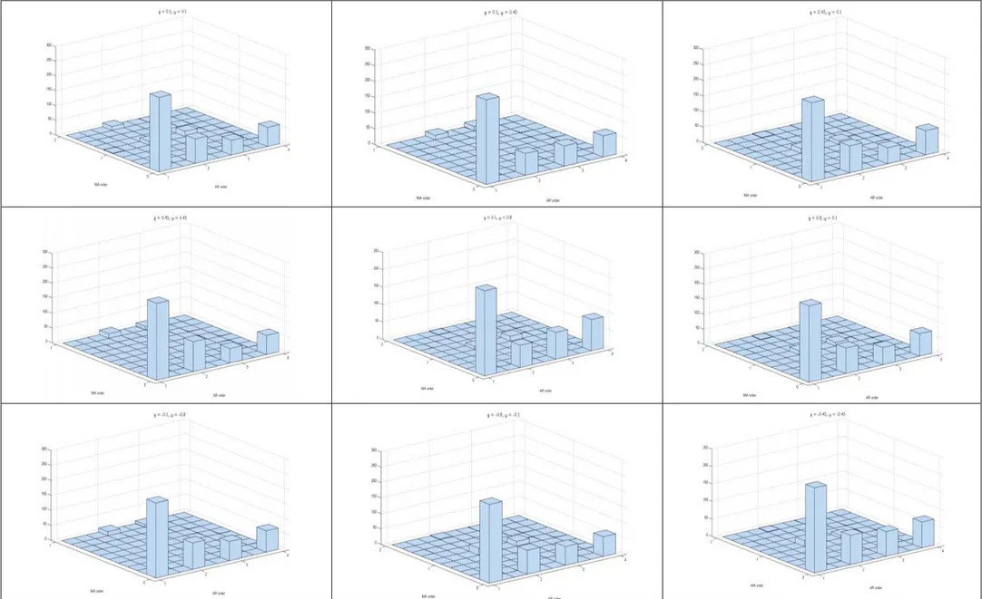
Finally, it may be of interest to look more closely at the results obtained under the poolability condition. In Figure 6 we have reported the ARMA orders estimated for the aggregated process

(scenario f1) when k =4 (the only value of k for which poolability holds true) and in Figure 7 we

show the estimate of φ ψ+ , which has been shown to be the parameter of the AR(1) model for the

aggregate when the poolability condition holds true. From both figures it can be seen that, as expected, the most frequently identified model is by far the AR(1) model (Figure 6). Moreover, the estimators appear to be consistent (Figure 7). It should be noted, however, that this does not give any advantage in terms of prediction accuracy, because the ranking of the forecasting performances

when the poolability condition holds (that is, when k =4), is approximately the same as the one

0.05 0.1 0.15 0 50 100 φ = 0.1, ψ = 0.1 0.05 0.1 0.15 0 50 100 φ = 0.1, ψ = 0.45 0.4 0.42 0.44 0.46 0.48 0.5 0 50 100 φ = 0.45, ψ = 0.1 0.4 0.42 0.44 0.46 0.48 0.5 0 50 100 φ = 0.45, ψ = 0.45 0.05 0.1 0.15 0 50 100 φ = 0.1, ψ = 0.8 0.75 0.8 0.85 0 50 100 φ = 0.8, ψ = 0.1 -0.16 -0.14 -0.12 -0.1 -0.08 -0.060 50 100 φ = -0.1, ψ = -0.8 -0.85 -0.8 -0.75 0 50 100 φ = -0.8, ψ = -0.1 -0.5 -0.48 -0.46 -0.44 -0.42 -0.4 0 50 100 φ = -0.45, ψ = -0.45

0.05 0.1 0.15 0 50 100 φ = 0.1, ψ = 0.1 0.4 0.42 0.44 0.46 0.48 0.5 0 50 100 φ = 0.1, ψ = 0.45 0.05 0.1 0.15 0 50 100 φ = 0.45, ψ = 0.1 0.4 0.42 0.44 0.46 0.48 0.5 0 50 100 φ = 0.45, ψ = 0.45 0.75 0.8 0.85 0 50 100 φ = 0.1, ψ = 0.8 0.05 0.1 0.15 0 50 100 φ = 0.8, ψ = 0.1 -0.85 -0.8 -0.75 0 50 100 φ = -0.1, ψ = -0.8 -0.16 -0.14 -0.12 -0.1 -0.08 -0.060 50 100 φ = -0.8, ψ = -0.1 -0.5 -0.48 -0.46 -0.44 -0.42 -0.4 0 50 100 φ = -0.45, ψ = -0.45

Figure 6: Joint frequency distributions of the estimated ARMA orders pˆ and qˆ in the f1 (aggregate) approach when the poolability condition holds (i.e., when k=4) and all

0.1 0.12 0.14 0.16 0.18 0.2 0.22 0.24 0.26 0.28 0.3 0 10 20 30 40 50 60 φ = 0.1, ψ = 0.1 0.46 0.48 0.5 0.52 0.54 0.56 0.58 0.6 0.62 0.64 0 10 20 30 40 50 60 70 φ = 0.1, ψ = 0.45 0.46 0.48 0.5 0.52 0.54 0.56 0.58 0.6 0.62 0.64 0 10 20 30 40 50 60 70 80 90 φ = 0.45, ψ = 0.1 0.8 0.82 0.84 0.86 0.88 0.9 0.92 0.94 0.96 0.98 1 0 10 20 30 40 50 60 70 80 φ = 0.45, ψ = 0.45 0.8 0.82 0.84 0.86 0.88 0.9 0.92 0.94 0.96 0.98 1 0 10 20 30 40 50 60 70 80 90 φ = 0.1, ψ = 0.8 0.8 0.82 0.84 0.86 0.88 0.9 0.92 0.94 0.96 0.98 1 0 10 20 30 40 50 60 70 φ = 0.8, ψ = 0.1 -1 -0.98 -0.96 -0.94 -0.92 -0.9 -0.88 -0.86 -0.84 -0.82 -0.8 0 10 20 30 40 50 60 70 80 φ = -0.1, ψ = -0.8 -1 -0.98 -0.96 -0.94 -0.92 -0.9 -0.88 -0.86 -0.84 -0.82 -0.8 0 10 20 30 40 50 60 70 φ = -0.8, ψ = -0.1 -1 -0.98 -0.96 -0.94 -0.92 -0.9 -0.88 -0.86 -0.84 -0.82 -0.8 0 10 20 30 40 50 60 70 φ = -0.45, ψ = -0.45

5. Multivariate aggregate forecasting from a STAR model

We now turn to consider the problem of aggregating a space–time series of a given spatial

dimension (say n) into a space–time series of smaller dimension (say k<n). The problem has a

very well grounded empirical motivation. For instance in the EU we often have the necessity of forecasting economic series at a NUTS2 level (regions), but we have in hand data also at a finer resolution (NUTS3 level or sub–regions). The choice is therefore between the strategy of forecasting the NUTS3 data and then aggregate them at a NUTS2 level or conversely the opposite criterion of aggregating the data at the NUTS2 level and then forecast the resulting space–time series (Andreano and Savio, 2005).

In presenting the simulation results we will consider some modifications of the setup used in the previous section in order to take into account the peculiarity of the new problem.

First of all we considered the spatial dimension as fixed and restricted ourselves only to the case of a 16–by–16 regular square lattice grid then aggregated onto an 8–by–8 grid (see Figure 8). Indeed, k = 64 is the maximum dimension that we are able to handle due to memory limitations. Furthermore, since we want to observe the spatial correlation properties of the forecasting error on the aggregated map, looking at smaller dimensions (e.g. an 8–by–8 grid then aggregated into a 4– by–4 grid) would involve the computation of a spatial correlation index on only 16 spatial observations and this would be dominated by edge effects and would make a lot less sense.

Secondly, we considered the same combinations of parameters used in Section 4, but we extended the cases of negative parameters with the introduction of three additional configurations:

the pairs

(

)

(

)

(

)

the experiments discussed in the previous section because of the symmetry that we observed between positive and negative values in terms of the MSE of the forecast.

Thirdly, since now we evaluate the forecasting error of a space–time series, the MSE alone is not a good measure of accuracy. In fact, when dealing with spatial data, not only a forecast is accurate when it produces a small MSE, but also when it preserves the spatial characteristics of the true data. In this second respect we consider accurate a forecast when it displays a spatial correlation that is similar to the spatial correlation of the original set of data, or, in other words, when the spatial correlation of the forecast error map is not significantly different from zero. Indeed, when the map of the forecast errors displays clusters of similar values, entire characteristics of the true series are cancelled; on the contrary when errors are randomly distributed in space, they are easier to detect and to be removed e. g. with the use of a spatial filtering (Arbia et al. 1999). We measure the spatial correlation in the true map, in the forecasted map and in the error map with the Moran’s I coefficient (Cliff and Ord, 1981) and we refer to the three cases with the symbols

It, If and Ife, respectively.

Finally, all the forecasting scenarios considered in Section 4 are considered again in the present section, but with some remarkable qualifications. In fact, Scenario f1 is no more relevant because it is intrinsically linked to the univariate forecasting criterion. When dealing with Scenario f2 we refer to the aggregated 8–by–8 spatial scheme and we fit a univariate ARMA to each series thus obtaining 64 forecasted values. We then compute the MSE for each of the 64 regions based on the out–of–sample observations. The Moran’s I coefficient is finally computed at each moment of time on the true map, on the forecasted map and on their difference (the error map). In the case of Scenario f3 we proceed in a similar fashion and we produce a forecast based on a 8–by–8 aggregated spatial scheme and with the parameter estimation based on a VAR(1) model. With respect to Scenario f3new we do not have any difference with respect to section 4: this scenario is just equivalent to Scenario f3, but with the constraint that the parameters that are not significant are set to zero in the estimation phase. Finally, as for Scenario f4 the estimation is obtained jointly for all locations in the spatial scheme based on a STAR(1,1) model which can also be viewed as a restricted VAR(1). We then proceed as in the other scenarios to compute the error maps and the associated MSE’s and Moran’s I tests.

16–by–16 Input data

Comparison between the two maps in terms of the MSE and in terms of the Moran’s

I test

8–by–8 Aggregated input data 8–by–8 Aggregate forecast map

Figure 8: Reference aggregation scheme for the new experiment designs.

Let us start by considering the spatial structure of the error map. As we have already remarked a desirable feature of the forecast is to reproduce most of the original spatial structure measured in terms of the Moran’s I coefficient. Hence the difference between the true and the forecasted map should contain no extra spatial correlation and the null of no spatial correlation should be accepted in the error map. A first synthesis of the large output obtained is reported in Figure 9. Here we consider, for each scenario and for each combination of the parameters, the number of cases in the 100 out–of–sample forecasts in which the null of zero spatial correlation is rejected at a significance level of 5 %. To facilitate the visualization we ordered the parameters’ values in increasing sense

with respect to the spatial parameter ψ . The values reported in each graph represent the mean of I

Moran’s values.

The analysis of Figure 9 reveals that the percentage of cases leading to rejection of the null hypothesis is very low in all scenarios and for any combination of the parameters. However it is always equal to zero in the case of Scenario f4. This means that if we use the STAR modelling framework the forecasting map presents spatial features that are very similar to those of the original data and thus the error map has the desirable feature of being spatially uncorrelated.

Table 4 reports, for each parameter combinations and for each scenario, the linear correlation between Moran’s I of the true map and the Moran’s I computed in the 100 out–of–sample forecasted maps. A similar table is reported in Table 5 which refers to the linear correlation between the true map Moran’s I and the error map Moran’s I.

The exam of Table 4 reveals that the highest value of the linear correlation is observed in Scenario f4. We can therefore conclude that, in this instance, the resulting forecasted spatial structure is very similar to the original one. Notice that, quite surprisingly, the highest levels of

similarity in all scenarios are achieved in cases of high temporal dependence (φ = 0.8 ) or in cases

Conversely, the lowest level of similarity (correlation close to zero) is observed in cases of low

temporal dependence, when φ = ±0.1 is associated to low spatial correlation in the true map. Notice

also the symmetry of the results for positive and negative values of the parameters. These results seem to suggest the dominance of the temporal aspects on the good performances of the forecasting scenarios when the aim consists in reproducing the spatial structure of the phenomenon. Comparatively less important appears to be the intensity of the spatial dependence in the original map under this respect.

(-0.1,-0.8)(-0.1,-0.45)(-0.45,-0.45)(-0.8,-0.1)(-0.45,-0.1)(-0.1,-0.1)(0.1,0.1)(0.45,0.1)(0.8,0.1)(0.1,0.45)(0.45,0.45)(0.1,0.8) -0.01 0 0.01 0.02 0.03 0.04 0.05

Percentage of rejection of the null hypothesis - scenario 2

(-0.1,-0.8)(-0.1,-0.45)(-0.45,-0.45)(-0.8,-0.1)(-0.45,-0.1)(-0.1,-0.1)(0.1,0.1)(0.45,0.1)(0.8,0.1)(0.1,0.45)(0.45,0.45)(0.1,0.8) -0.01 0 0.01 0.02 0.03 0.04 0.05

Percentage of rejection of the null hypothesis - scenario 3

(-0.1,-0.8)(-0.1,-0.45)(-0.45,-0.45)(-0.8,-0.1)(-0.45,-0.1)(-0.1,-0.1)(0.1,0.1)(0.45,0.1)(0.8,0.1)(0.1,0.45)(0.45,0.45)(0.1,0.8) -0.01 0 0.01 0.02 0.03 0.04 0.05

Percentage of rejection of the null hypothesis - scenario 3new

(-0.1,-0.8)(-0.1,-0.45)(-0.45,-0.45)(-0.8,-0.1)(-0.45,-0.1)(-0.1,-0.1)(0.1,0.1)(0.45,0.1)(0.8,0.1)(0.1,0.45)(0.45,0.45)(0.1,0.8) -0.01 0 0.01 0.02 0.03 0.04 0.05

Percentage of rejection of the null hypothesis - scenario 4

True data Forecasts Forecast errors True data Forecasts Forecast errors True data Forecasts Forecast errors True data Forecasts Forecast errors

Figure 9: Percentage of rejection of the null hypothesis of zero spatial correlation at α = 0.05 confidence level in the

various scenarios. In the vertical axes we report the quantities 300 { }

1 # t 0, 0.05 , _i i I α φ ψ = ≠ = ∑ , 300 { } 1 # f 0, 0.05 , _i i I α φ ψ = ≠ = ∑ and { } 300 1 # ef 0, 0.05 , _i i I α φ ψ = ≠ =

∑ respectively. For each test we considered the z–scores with E I( )l = −

1 n− 1 and Var I( )l = 2 wij j ∑ i ∑ (with l= t, f , fe).

Moving to commenting Table 5 we notice very low values of the linear correlation between the true map Moran’s I and the error map Moran’s I in the case of Scenario f4. This seems to confirm the previous finding of the superiority of Scenario f4 when we look at the spatial properties of errors, and of the dominance of temporal aspects with respect to spatial characteristics of the original data. It is particularly evident the inability of Scenario f2 under this respect where we record high and positive values of the correlation: in cases when the original data are characterized by high levels of spatial correlation, the error maps still preserves the same feature.

To reinforce these conclusions let us look at Figure 10 which reports the absolute values of the Moran’s I coefficients in all scenarios and for all combination of parameters, for the true data, the forecast map and the error map. In the case of Scenario f2 the error map has always a similar spatial structure with respect to the original map. In the cases of Scenario f3 and f3new we observe an over–fitting. When the original data are characterised by positive spatial correlation we observe a negative spatial correlation in the error map especially in the cases of very strong spatial correlation

(the two extreme cases of ψ = ±0.8 ). Finally Scenario f4 leads also to an over–fitting, but constantly on negative values very close to zero in absolute value.

For the computation of the MSE’s characterising each scenario and each parameter combinations we consider the average of the 100 MSE associated to each of the out–of–sample forecasting values and we average them over the 300 replications. Figure 11 reports the results obtained.

Scenario f4 dominates all other strategies in that it consistently achieves the lowest MSE’s in all combinations of parameters. The advantage of using a forecasting strategy based on the STAR modelling framework is particularly evident with respect to scenario f2 and f3 and in those

instances dominated by a high temporal correlation where φ = ±0.8.

In order to visualize jointly the a–spatial characteristics of errors (measured by the MSE) and their spatial features (measured by Moran’s I statistics), Figure 12 reports the scatterplot of these two aspects with reference to the forecasting error maps.

f2 f3 f3new f4 (–0.1, –0.8) 0.4524 0.5522 0.6921 0.6201 (–0.1, –0.45) 0.0788 –0.0288 0.0418 0.1594 (–0.45, –0.45) 0.2581 0.4965 0.7224 0.8309 (–0.8, –0.1) 0.0896 0.3320 0.7204 0.9526 Numerical (–0.45, –0.1) 0.1120 0.0879 0.3405 0.4201 value of the (–0.1, –0.1) 0.0681 –0.0287 –0.0720 0.1212 parameters (0.1, 0.1) 0.0159 –0.0631 0.0725 0.0624 (φ,ψ) (0.45, 0.1) 0.0580 0.0735 0.3442 0.4945 (0.8, 0.1) 0.1029 0.3037 0.6767 0.9395 (0.1, 0.45) 0.0919 –0.0840 0.0619 0.1982 (0.45, 0.45) 0.3618 0.4471 0.7246 0.7585 (0.1, 0.8) 0.3865 0.6280 0.7000 0.5979

Table 4: Correlation between the I–Moran values in the true map (It) and the I–Moran in the forecast map (If) for

each combination of the parameters ( )φ,ψ and for each forecasting scenario. The highest values are highlighted in

boldface. f2 f3 f3new f4 (–0.1, –0.8) 0.7539 0.1467 0.4857 0.0688 (–0.1, –0.45) 0.8374 0.4902 0.7526 –0.0157 (–0.45, –0.45) 0.6547 0.3592 0.5079 0.0406 (–0.8, –0.1) 0.5358 0.2727 0.4155 –0.0747 Numerical (–0.45, –0.1) 0.8202 0.4050 0.6364 –0.0702 Value of the (–0.1, –0.1) 0.8324 0.5821 0.8082 0.0235 parameters (0.1, 0.1) 0.8206 0.5478 0.8258 –0.0332 (φ,ψ) (0.45, 0.1) 0.7735 0.4424 0.6174 –0.0960 (0.8, 0.1) 0.5331 0.2628 0.3761 –0.0144 (0.1, 0.45) 0.8201 0.5443 0.7771 –0.0869 (0.45, 0.45) 0.6920 0.3070 0.4968 –0.0131 (0.1, 0.8) 0.7086 0.3192 0.4984 –0.0209

Table 5: Correlation between the I–Moran values in the true map (It) and the I–Moran in the error map (I ) for each fe

(-0.1,-0.8) (-0.1,-0.45) (-0.45,-0.45) (-0.8,-0.1) (-0.45,-0.1)(-0.1,-0.1) (0.1,0.1)(0.45,0.1) (0.8,0.1)(0.1,0.45)(0.45,0.45)(0.1,0.8) -0.02 -0.01 0 0.01 0.02 0.03 0.04

0.05 Values of Moran index - scenario 2

(-0.1,-0.8) (-0.1,-0.45) (-0.45,-0.45) (-0.8,-0.1) (-0.45,-0.1) (-0.1,-0.1)(0.1,0.1) (0.45,0.1) (0.8,0.1)(0.1,0.45)(0.45,0.45)(0.1,0.8) -0.04 -0.03 -0.02 -0.01 0 0.01 0.02

0.03 Values of Moran index - scenario 3

(-0.1,-0.8) (-0.1,-0.45) (-0.45,-0.45) (-0.8,-0.1) (-0.45,-0.1)(-0.1,-0.1) (0.1,0.1)(0.45,0.1) (0.8,0.1)(0.1,0.45)(0.45,0.45)(0.1,0.8) -0.03 -0.02 -0.01 0 0.01 0.02 0.03

0.04 Values of Moran index - scenario 3new

(-0.1,-0.8) (-0.1,-0.45) (-0.45,-0.45) (-0.8,-0.1) (-0.45,-0.1)(-0.1,-0.1) (0.1,0.1)(0.45,0.1) (0.8,0.1)(0.1,0.45)(0.45,0.45) (0.1,0.8) -0.04 -0.02 0 0.02 0.04 0.06 0.08 0.1 0.12 0.14

0.16 Values of Moran index - scenario 4 True data Forecasts Forecast errors True data Forecasts Forecast errors True data Forecasts Forecast errors True data Forecasts Forecast errors

Figure 10: Values of Moran’s I coefficient in the true maps, in the forecasted maps and in the error maps, for all

combinations of parameters ( )φ,ψ (φ = temporal parameter, ψ = spatial parameter) and for each forecasting scenario.

(-0.1,-0.8) (-0.1,-0.45) (-0.45,-0.45) (-0.8,-0.1) (-0.45,-0.1) (-0.1,-0.1) (0.1,0.1) (0.45,0.1) (0.8,0.1) (0.1,0.45) (0.45,0.45) (0.1,0.8) 200 300 400 500 600 700 800 900 1000 1100

Average MSE in the four scenarios Univariate

VAR RVAR STAR

Figure 11: MSE of the four forecasting scenarios for all combinations of parameters (φ ψ (φ = temporal parameter, ψ , )

-0.02 -0.01 0 0.01 0.02 200 400 600 800 1000 1200 I fe MS E

Scatterplot of I_fe vs. MSE - scenario 2

-0.015 -0.01 -0.005 0 0.005 0.01 0.015 0.02 0.025 200 300 400 500 600 700 I fe MS E

Scatterplot of I_fe vs. MSE - scenario 3

-0.02 -0.01 0 0.01 0.02 0.03 0.04 220 240 260 280 300 320 I fe MS E

Scatterplot of I_fe vs. MSE - scenario 3new

0 0.02 0.04 0.06 0.08 0.1 0.12 0.14 0.16 190 200 210 220 230 240 I fe MS E

Scatterplot of I_fe vs. MSE - scenario 4

(-0.1,-0.8) (-0.1,-0.45) (-.045,-0.45) (-0.8,-0.1) (-0.45,-0.1) (-0.1,-0.1) (0.1,0.1) (0.45,0.1) (0.8,0.1) (0.1,0.45) (0.45,0.45) (0.1,0.8) (-0.1,-0.8) (-0.1,-0.45) (-.045,-0.45) (-0.8,-0.1) (-0.45,-0.1) (-0.1,-0.1) (0.1,0.1) (0.45,0.1) (0.8,0.1) (0.1,0.45) (0.45,0.45) (0.1,0.8) (-0.1,-0.8) (-0.1,-0.45) (-.045,-0.45) (-0.8,-0.1) (-0.45,-0.1) (-0.1,-0.1) (0.1,0.1) (0.45,0.1) (0.8,0.1) (0.1,0.45) (0.45,0.45) (0.1,0.8) (-0.1,-0.8) (-0.1,-0.45) (-.045,-0.45) (-0.8,-0.1) (-0.45,-0.1) (-0.1,-0.1) (0.1,0.1) (0.45,0.1) (0.8,0.1) (0.1,0.45) (0.45,0.45) (0.1,0.8)

Figure 12: Scatterplot of Moran’s I coefficient on the error map versus the MSE of the same map for each forecasting scenario.

In this graph, points close to zero in both coordinates represent the ideal instances of forecast where both the MSE is low and Moran’s I is close to zero.

The visual inspection of this graph generally confirms the marked superiority of the STAR modelling framework with respect to the other startegies. More in detail, scenario f2 produces forecasts that are rather accurate in terms of the map structure, but highly inaccurate in terms of the

MSE when

(

)

(

)

and temporal correlation. Conversely it produces low MSE’s, but negative spatial and temporal correlation in the errors in the cases of moderate spatial and temporal parameters, i.e.

(

)

A similar result is obtained with scenario f3 and f3new, but with lower absolute MSE’s. Figure 12 (scenario f4) finally points out that the most accurate forecasts are produced for the

combinations of parameters

(

)

most cases of low absolute spatial correlation.

6. Summary and final comments

The aim of this paper was to perform a thorough comparison of the relative efficiency of different methods of forecasting data that are both temporally and spatially correlated. We started by looking at the situation of a space–time series aggregated into a single time series. This situation was already examined by GG, but we extended their findings by examining larger datasets to check the dependence of results on the spatial dimension, by introducing the case of negative spatial correlation and by explicitly considering the problem of edge effects in the phase

of simulation. We then moved to evaluate the performances of various forecasting strategies in cases where we aggregate a fine grid of space–time data into a coarser space–time series.

The first part of the paper generalizes the findings of GG in showing that most of the times the worst performing methods are the aggregation of univariate forecasts (Scenario f2) and Scenario f3 (unrestricted VAR). In small and medium–sized spatial schemes scenario f2 presents the worst performances in the case of strong spatial dependence. For high spatial dimensions, conversely, scenario f3 always performs the worst. Furthermore, from our simulations we stress the fact that, in terms of forecasting efficiency, a correct specification of the model is of paramount importance

when the spatial dependence parameter ψ is high in absolute value. In particular we have shown

that Scenario f4, based on the STAR methodology, guarantees a good improvement of the forecasting efficiency in terms of the MSE when moving from small to high absolute values of spatial correlation. However the spatial dimension plays an important role and the percentage of cases in which Scenario f4 outperforms the other forecasting methods increases with the number of regions up to a dimension of k = 49 and then it decreases again.

Finally the simulation experiments show clearly that spatial dependence has a relevant impact on the choice of the forecasting method no matter what is its sign. When spatial dependence is weak in absolute value, the ranking of the models is mostly related to the number of regions. Conversely when spatial dependence increases, this ranking is essentially independent of the dimension of the grid and it is strictly related to the strength of spatial dependence.

In the second part of the paper we moved to consider the more general case of space–time series from a fine into a coarser disaggregation. For instance, suppose that we have in hand a space–time series of economic data collected at a given level of spatial disaggregation (e.g. sub– national regions at the EU level). If the aim is to forecast the series at a national level starting from this set of information we may employ different strategies similar to those examined before, but with a remarkable difference. In this case the outcome of the aggregation procedure, in fact, is not merely a time series of data, but it is a new space–time series. In these conditions a forecasting strategy has to be judged not only in terms of the standard MSE measure, but also in terms of the spatial characteristics of the forecasting errors. In fact we expect a good forecasting strategy to be characterized by a small MSE and also by the ability to reproduce the characteristics of spatial dependence of the original data. Indeed a forecasting method that provides an accurate estimate in terms of MSE may well be rejected if it provides forecasting errors that are concentrated in a systematic way in some definite portions of space thus displaying a positive spatial correlation. Throughout the paper we employ Moran’s I spatial correlation coefficient to quantify this second, important, characteristics of forecasting errors.

Under this second respect our simulations show quite clearly that the best strategy both in terms of the minimum MSE and in terms of the smallest Moran’s I is, in all cases examined, the

STAR modelling (Scenario f4). In fact this strategy dominates all other forecasting procedures in

terms of the MSE, produces the lowest I–Moran of the error map, thus showing its ability to reconstruct pretty well the original map structure. Indeed the spatial properties of data are better preserved in the forecasted data in cases of high temporal (positive or negative) correlation whereas the level of spatial correlation in the true data map appears to be less relevant under this respect. When the spatial correlation parameter is close to zero in absolute value f4 scenario is able to produce both low MSE’s and spatial correlation close to zero.

Our conclusions thus extend those obtained by GG to a more general setup: we have shown that in most empirical cases it is better to forecast a space–time series with a STAR model and then aggregate the forecast. The paper also highlights how the gain in efficiency is related to the spatial dimension and to the absolute values of the temporal and spatial coefficient. In this respect the results reported here can be of help in assisting the choice between the various forecasting alternatives in empirical circumstances.

References

Andreano M.S., Savio G. (2005) Aggregation of space–time processes: indirect or direct approaches for forecasting economic aggregates?, Euronews Indicators, Eurostat, Luxembourg, June. Arbia G. (2006) Spatial Econometrics: Statistical Foundations and Applications to regional

Convergence, Springer Verlag, Berlin.

Arbia G., Benedetti R., Espa G. (1999) Classification in image analysis: an assessment of accuracy of ICM, Computational Statistics and Data Analysis, 30, 4, 443–455.

Besag J. (1974) Spatial Interaction and the Statistical Analysis of Lattice Systems (with discussion),

Journal of the Royal Statistical Society, B, 36, 192–236.

Cliff A.D., Ord J.K. (1981) Spatial processes. Models and applications, Pion, London.

Cliff A.D., Haggett P., Ord J.K., Bassett K., Davies R. (1975) Elements of Spatial Structure – A

Quantitative Approach, Cambridge University Press, Cambridge.

Giacomini R., Granger C.W.J. (2004) Aggregation of space–time processes, Journal of

Econometrics, 118, 7–26.

Griffith A.D. (1983) The boundary value problem in spatial statistical analysis, Journal of Regional

Science, 23, 377–387.

Griffith A.D. (1985) An evaluation of correction techniques for boundary effects in spatial statistical analysis: contemporary methods, Geographical Analysis, 17, 81–88.

Griffith A.D. (1988) Advanced spatial statistics, Kluwer Academic Press, Dordrecht.

Griffith A.D. (2006) Hidden negative spatial autocorrelation, Journal of Geographical Systems, 8,

335–355.

Griffith A.D., Arbia G. (2006) Effects of negative spatial autocorrelation in linear regression modelling, Paper presented at the International Workshop on Spatial Econometrics and

Statistics, Rome, May 2006.

Kohn R. (1982) When is an aggregate of a time series efficiently forecast by its past?, Journal of

Econometrics, 18, 337–350.

Lütkepohl H. (1987) Forecasting aggregated vector ARMA processes, Springer Verlag, Berlin. Lütkepohl H. (1993) Introduction to Multiple Time Series Analysis, Springer Verlag, Berlin.

Pfeifer P.E., Deutsch S.J. (1980) A three–stage iterative procedure for space–time modeling,

Technometrics, 22, 35–47.

Ripley B.D. (1981) Spatial Statistics, Wiley, New York.

Schwarz G. (1978) Estimating the Dimension of a Model, Annals of Statistics, 6, 461–464.

Upton G.J.G., Fingleton B. (1985) Spatial Data Analysis by Example. Vol. 1: Point pattern and

! " # $ % " ! " & ! ! ' ( ! ) * + , * - -. / # ! - . ! 0 - ) # ! ! $ 1 / 1 % & + 0 ' # ! . / # " ( ) * % & $ 2 ) ! " 1 % . % 1 # ! " / / ' ! * ' ! % ( ! ) $ ) $ 3 4 5 4 5 . ! % & 1 6 ( ( ( 7899 789: $ %

' ($ 0 ( ; < $ $ = + 1 . % 1 . + , $ - . 1 0 ! " ! = $ + . / 0* $ + . / 1 1 ( - . % +2 3 - 4/ # $ % & 1 # 3 - . - ( 5 6 $ ' 1 ! ) . ' + 2 + " * . ' . ! * - 7 8 ) 9 . ' 0 + ' * . 7 8 ) : ' $ " ) / " % ) = ! " 0 ! " 1 > ! " &" " 6 $ " ' %-* & ' * # - #- -$ + 2 /