Practical temperature Measurement

Practical

Temperature

Measurements

Application Note 290

Introduction 2 The Thermocouple 4 Practical Thermocouple 11 Measurements The RTD 18 The Thermistor 22 Monolithic Linear 23 Temperature Sensor

The Measurement System 24

Appendix A 27

Appendix B 28

Thermocouple Hardware 30

Bibliography 31

The purpose of this application note is to explore the more common temperature measurement techniques, and introduce procedures for

improving their accuracy.

We will focus on the four most com-mon temperature transducers: the thermocouple, the RTD (Resistance Temperature Detector), the thermistor and the integrated circuit sensor. Despite the widespread popularity of the thermocouple, it is frequently misused. For this reason, we will concentrate primarily on thermo-couple measurement techniques. Appendix A contains the empirical laws of thermocouples which are the basis for all derivations used herein. Readers wishing a more thorough discussion of thermocouple theory are invited to read reference 3 in the Bibliography.

For those with a specific thermo-couple application, Appendix B may aid in choosing the best type of thermocouple.

Throughout this application note we will emphasize the practical considera-tions of transducer placement, signal conditioning and instrumentation.

Early Measuring Devices

Galileo is credited with inventing the thermometer, circa 1592.1,2 _{In an open}

container filled with colored alcohol, he suspended a long narrow-throated glass tube, at the upper end of which was a hollow sphere. When heated, the air in the sphere expanded and bubbled through the liquid. Cooling the sphere caused the liquid to move up the tube.1_{Fluctuations in the}

temperature of the sphere could then be observed by noting the position of

the liquid inside the tube. This “upside-down” thermometer was a poor indicator since the level changed with barometric pressure, and the tube had no scale. Vast improvements were made in temperature measure-ment accuracy with the developmeasure-ment of the Florentine thermometer, which incorporated sealed construction and a graduated scale.

In the ensuing decades, many thermo-metric scales were conceived, all based on two or more fixed points. One scale, however, wasn’t universally recognized until the early 1700’s when Gabriel Fahrenheit, a Dutch instru-ment maker, produced accurate and repeatable mercury thermometers. For the fixed point on the low end of his temperature scale, Fahrenheit used a mixture of ice water and salt (or ammonium chloride). This was the lowest temperature he could repro-duce, and he labeled it “zero degrees.” For the high end of his scale, he chose human blood temperature and called it 96 degrees.

Why 96 and not 100 degrees? Earlier scales had been divided into twelve parts. Fahrenheit, in an apparent quest for more resolution divided his scale into 24, then 48 and eventually 96 parts.

The Fahrenheit scale gained populari-ty primarily because of the repeatabili-ty and qualirepeatabili-ty of the thermometers that Fahrenheit built.

Around 1742, Anders Celsius proposed that the melting point of ice and the boiling point of water be used for the two benchmarks. Celsius selected zero degrees as the boiling point and 100 degrees as the melting point. Later, the end points were reversed and the centigrade scale was born. In 1948 the name was officially changed to the Celsius scale.

In the early 1800’s William Thomson (Lord Kelvin), developed a universal thermodynamic scale based upon the coefficient of expansion of an ideal gas. Kelvin established the concept of absolute zero, and his scale remains the standard for modern thermometry. The conversion equations for the four modern temperature scales are: °C = 5/9 (°F - 32) °F = 9/5° C + 32

°k = °C + 273.15 °R = °F + 459.67 The Rankine Scale (°R) is simply the Fahrenheit equivalent of the Kelvin scale, and was named after an early pioneer in the field of thermodynam-ics, W. J. M. Rankine. Notice the official Kelvin scale does not carry a degree sign. The units are expressed in “kelvins,” not degrees Kelvin.

Reference Temperatures

We cannot build a temperature divider as we can a voltage divider, nor can we add temperatures as we would add lengths to measure distance. We must rely upon temperatures established by physical phenomena which are easily observed and consistent in nature. The International Temperature Scale (ITS) is based on such phenomena. Revised in 1990, it establishes seven-teen fixed points and corresponding temperatures. A sampling is given in Table 1.

Since we have only these fixed tem-peratures to use as a reference, we must use instruments to interpolate between them. But accurately interpo-lating between these temperatures can require some fairly exotic transducers, many of which are too complicated or expensive to use in a practical situa-tion. We shall limit our discussion to the four most common temperature transducers: thermocouples, resist-ance-temperature detector’s (RTD’s), thermistors, and integrated circuit sensors.

Table 1

ITS-90 Fixed Points

Temperature

Element Type K °C

(H₂) Hydrogen Triple Point 13.8033 K -259.3467° C

(Ne) Neon Triple Point 24.5561 K -248.5939 ° C

(0₂) Oxygen Triple Point 54.3584 K -218.7916° C

(Ar) Argon Triple Point 83.8058 K -189.3442° C

(Hg) Mercury Triple Point 234.315 K -38.8344° C

(H₂O) Water Triple Point 273.16 K +0.01° C

(Ga) Gallium Melting Point 302.9146 K 29.7646° C

(In) Indium Freezing Point 429.7485 K 156.5985° C

(Sn) Tin Freezing Point 505.078 K 231.928° C

(Zn) Zinc Freezing Point 692.677 K 419.527° C

(Al) Aluminum Freezing Point 933.473 K 660.323° C

(Ag) Silver Freezing Point 1234.93 K 961.78° C

(Au) Gold Freezing Point 1337.33 K 1064.18° C

Temperature Thermocouple V o lt age V T Resi st ance R T Resi st ance R T Vo lt age or Cur rent V or I T

Temperature Temperature Temperature Advantages ●_Self-powered Simple Rugged Inexpensive Wide variety of physical forms Wide temperature range ● ● ● ● ● Disadvantages ● ● ● ● ●_Non-linear Low voltage Reference required Least stable Least sensitive ●_Expensive Slow Current source required Small resistance change Four-wire measurement ● ● ● ● ●_Non-linear Limited temperature range Fragile Current source required Self-heating ● ● ● ● ●_{T < 250° C} Power supply required Slow Self-heating Limited configurations ● ● ● ● ●_{Most stable} Most accurate More linear than thermocouple ● ● ●_{High output} Fast Two-wire ohms measurement ● ● ●_{Most linear} Highest output Inexpensive ● ● Thermistor RTD I. C. Sensor

When two wires composed of dissimilar metals are joined at both ends and one of the ends is heated, there is a continuous current which flows in the thermoelectric circuit. Thomas Seebeck made this discovery in 1821 (Figure 2).

If this circuit is broken at the center, the net open circuit voltage (the Seebeck voltage) is a function of the junction temperature and the com-position of the two metals (Figure 3). All dissimilar metals exhibit this effect. The most common combina-tions of two metals are listed on page 28 of this application note, along with their important characteristics. For small changes in temperature the Seebeck voltage is linearly proportional to temperature: e_AB= αT

Where α, the Seebeck coefficient, is the constant of proportionality. (For real world thermocouples, αis not constant but varies with temperature. This factor is discussed under “Voltage-to-Temperature Conversion” on page 9.)

The Thermocouple

+

=

=

Measuring Thermocouple Voltage

We can’t measure the Seebeck voltage directly because we must first connect a voltmeter to the thermocouple, and the voltmeter leads, themselves, create a new thermoelectric circuit.

Let’s connect a voltmeter across a copper-constantan (Type T) thermo-couple and look at the voltage output (Figure 4).

We would like the voltmeter to read only V₁, but by connecting the volt-meter in an attempt to measure the output of Junction J₁we have created two more metallic junctions: J₂and J₃. Since J₃is a copper-to-copper junc-tion, it creates no thermal e.m.f. (V₃= 0) but J₂is a copper-to constan-tan junction which will add an e.m.f. (V₂) in opposition to V₁. The resultant voltmeter reading V will be propor-tional to the temperature difference between J₁and J₂. This says that we can’t find the temperature at J₁unless we first find the temperature of J₂.

The Reference Junction

One way to determine the temperature J₂is to physically put the junction into an ice bath, forcing its tempera-ture to be 0° C and establishing J₂as the Reference Junction. Since both voltmeter terminal junctions are now copper-copper, they create no thermal e.m.f. and the reading V on the voltmeter is proportional to the temperature difference between J₁ and J₂.

Now the voltmeter reading is (See Figure 5): V = (V₁– V₂) ≅ α(t J1– tJ2) If we specify T J1in degrees Celsius: T J1(°C) + 273.15 = tJ1(K) then V becomes: V = V₁– V₂= α[(T J1+ 273.15) – (TJ2+ 273.15)] = α(T J1– TJ2) = (TJ1– 0) V = αT J1

We use this protracted derivation to emphasize that the ice bath junction output V₂is not zero volts. It is a function of absolute temperature. By adding the voltage of the ice point reference junction, we have now referenced the reading V to 0° C. This method is very accurate because the ice point temperature can be precisely controlled. The ice point is used by the National Institute of Standards and Technology (NIST) as the fundamental reference point for their thermocouple tables, so we can now look at the NIST tables and directly convert from voltage V to Temperature T

J1.

The copper-constantan thermocouple shown in Figure 5 is a unique example because the copper wire is the same metal as the voltmeter terminals. Let’s use an iron-constantan (Type J) thermocouple instead of the copper-constantan. The iron wire (Figure 6) increases the number of dissimilar metal junctions in the circuit, as both voltmeter terminals become Cu-Fe thermocouple junctions.

This circuit will still provide moderate-ly accurate measurements as long as the voltmeter high and low terminals (J₃& J₄) act in opposition (Figure 7). If both front panel terminals are not at the same temperature, there will be an error. For a more precise measurement, the copper voltmeter leads should be extended so the copper-to-iron junctions are made on an isothermal (same temperature) block (Figure 8).

The isothermal block is an electrical insulator but a good heat conductor and it serves to hold J₃and J₄at the same temperature. The absolute block temperature is unimportant because the two Cu-Fe junctions act in opposition. We still have: V = α(T J1– TREF) Figure 8 Removing junctions from DVM terminals Figure 6 Iron Constantan couple Figure 5 External reference junction Figure 7 Junction voltage cancellation

=

Reference Circuit

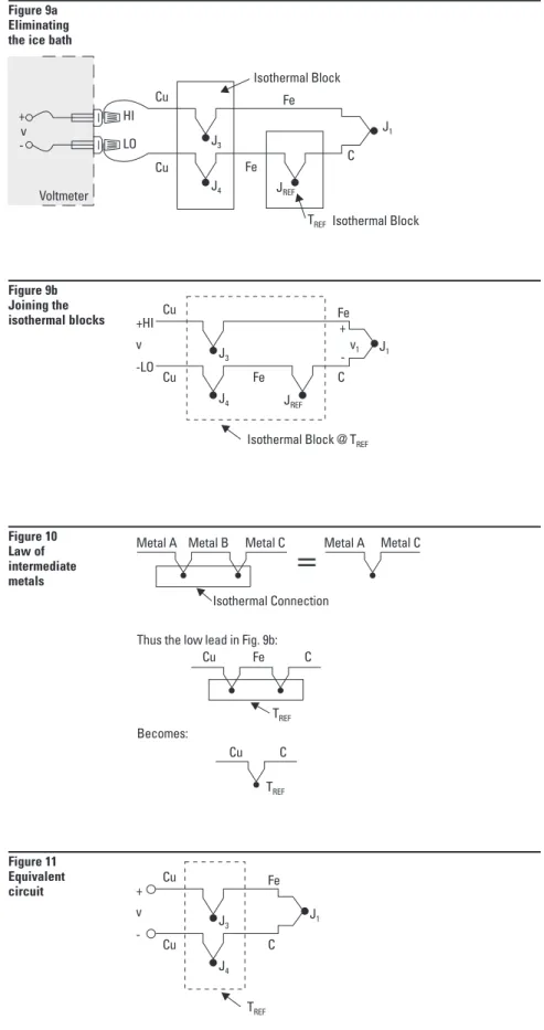
The circuit in Figure 8 will give us accurate readings, but it would be nice to eliminate the ice bath if possible. Let’s replace the ice bath with another isothermal block (Figure 9).

The new block is at Reference Temperature T_REF, and because J₃and J₄are still at the same temperature we can again show that: V = α(T₁– T_REF)

This is still a rather inconvenient circuit because we have to connect two thermocouples. Let’s eliminate the extra Fe wire in the negative (LO) lead by combining the Cu-Fe junction (J₄) and the Fe-C junction (J_REF).

We can do this by first joining the two isothermal blocks (Figure 9b). We haven’t changed the output voltage V. It is still:

V = α(T

J1– TREF)

Now we call upon the law of inter-mediate metals (see Appendix A) to eliminate the extra junction. This empirical law states that a third metal (in this case, iron) inserted between the two dissimilar metals of a thermo-couple junction will have no effect upon the output voltage as long as the two junctions formed by the additional metal are at the same temperature (Figure 10).

This is a useful conclusion, as it com-pletely eliminates the need for the iron (Fe) wire in the LO lead (Figure 11). Again V = α(T₁– T_REF) where αis the Seebeck coefficient for an Fe-C thermocouple.

Junctions J₃and J₄take the place of the ice bath. These two junctions now become the reference junction.

Figure 9a Eliminating the ice bath

Figure 9b Joining the isothermal blocks Figure 10 Law of intermediate metals Figure 11 Equivalent circuit C HI LO + -v Voltmeter J1 Fe Fe Cu Cu Isothermal Block J₃

TREFIsothermal Block

J₄ JREF C +HI -LO v v1 J1 Fe Fe Cu Cu J3

Isothermal Block @ TREF

J4 JREF + -C + -v J1 Fe Cu Cu J3 T_REF J4

=

Metal A Metal B Metal C Metal A Metal C

Isothermal Connection Thus the low lead in Fig. 9b:

Cu Becomes: Fe C T_REF Cu C TREF

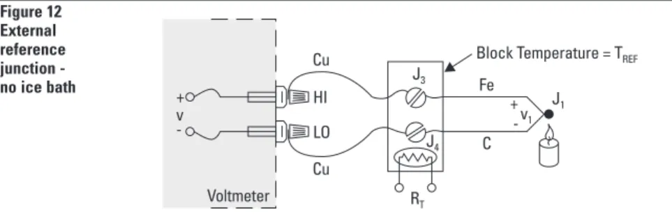
Now we can proceed to the next logical step: Directly measure the temperature of the isothermal block (the reference junction) and use that information to compute the unknown temperature, T

J1(Figure 12).

A thermistor, whose resistance R_Tis a function of temperature, provides us with a way to measure the absolute temperature of the reference junction. Junctions J₃and J₄and the thermistor are all assumed to be at the same temperature, due to the design of the isothermal block. Using a digital multimeter (DMM), we simply: 1. Measure R_Tto find T_REFand

convert T_REFto its equivalent reference junction voltage, V_REF 2. Measure V and add V_REFto find V₁

and convert V₁to temperature T

J1.

This procedure is known as

software compensationbecause it

relies upon software in the instrument or a computer to compensate for the effect of the reference junction. The isothermal terminal block temperature sensor can be any device which has a characteristic proportional to absolute temperature: an RTD, a thermistor, or an integrated circuit sensor.

It seems logical to ask: If we already have a device that will measure absolute temperature (like an RTD or thermistor), why do we even bother with a thermocouple that requires reference junction compensation? The single most important answer to this question is that the thermistor, the RTD, and the integrated circuit trans-ducer are only useful over a certain temperature range. Thermocouples, on the other hand, can be used over a range of temperatures, and optimized for various atmospheres. They are much more rugged than thermistors, as evidenced by the fact that thermo-couples are often welded to a metal part or clamped under a screw. They can be manufactured on the spot, either by soldering or welding. In short, thermocouples are the most versatile temperature transducers available and since the measurement

Figure 12 External reference junction - no ice bath C J₄ J₃ HI LO + -v Voltmeter J1 R_T Fe Cu

Cu Block Temperature = TREF

+

-v1

reference compensation and software voltage-to-temperature conversion, using a thermocouple becomes as easy as connecting a pair of wires.

Thermocouple measurement becomes especially convenient when we are required to monitor a large number of data points. This is accomplished by using the isothermal reference junction for more than one thermo-couple element (Figure 13). A relay scanner connects the voltmeter to the various thermocouples in sequence. All of the voltmeter and scanner wires are copper, independent of the type of thermocouple chosen. In fact, as long as we know what each thermocouple is, we can mix thermocouple types on the same isothermal junction block (often called a zone box) and make the appropriate modifications in soft-ware. The junction block temperature sensor, R_Tis located at the center of the block to minimize errors due to thermal gradients.

Software compensation is the most versatile technique we have for measuring thermocouples. Many thermocouples are connected on the same block, copper leads are used throughout the scanner, and the tech-nique is independent of the types of thermocouples chosen. In addition, when using a data acquisition system with a built-in zone box, we simply connect the thermocouple as we would a pair of test leads. All of the conversions are performed by the instrument’s software. The one disadvantage is that it requires a small amount of additional time to calculate the reference junction temperature. For maximum speed we can use hardware compensation. Figure 13 Switching multiple thermocouple types + -v Voltmeter R_T Pt Pt - 10%Rh Isothermal Block (Zone Box) C Fe

All Copper Wires HI

Hardware Compensation

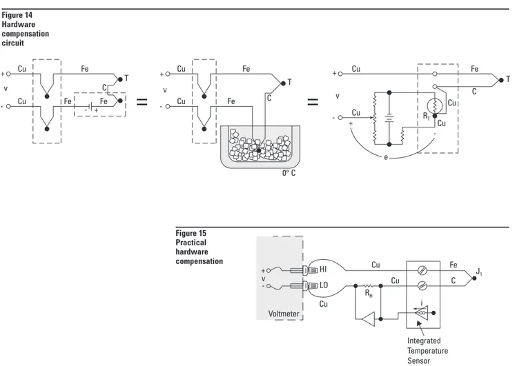
Rather than measuring the tempera-ture of the reference junction and computing its equivalent voltage as we did with software compensation, we could insert a battery to cancel the offset voltage of the reference junc-tion. The combination of this hard-ware compensation voltage and the reference junction voltage is equal to that of a 0° C junction (Figure 14). The compensation voltage, e, is a function of the temperature sensing resistor, R_T. The voltage V is now referenced to 0° C, and may be read directly and converted to temperature by using the NIST tables.

Another name for this circuit is the

electronic ice point reference.6 These

circuits are commercially available for use with any voltmeter and with

Figure 14 Hardware compensation circuit Figure 15 Practical hardware compensation

=

=

a wide variety of thermocouples. The major drawback is that a unique ice point reference circuit is usually needed for each individual thermo-couple type.

Figure 15 shows a practical ice point reference circuit that can be used in conjunction with a relay scanner to compensate an entire block of thermo-couple inputs. All the thermothermo-couples in the block must be of the same type, but each block of inputs can accom-modate a different thermocouple type by simply changing gain resistors. The advantage of the hardware com-pensation circuit or electronic ice point reference is that we eliminate the need to compute the reference temperature. This saves us two com-putation steps and makes a hardware compensation temperature measure-ment somewhat faster than a software

compensation measurement. However, today’s faster microprocessors and advanced data acquisition designs continue to blur the line between the two methods, with software compensation speeds challenging those of hardware compensation in practical applications (Table 2).

Table 2 Hardware Software Compensation Compensation ●_Fast ●_{Restricted to one} themocouple type per reference junction ●_{Hard to reconfigure –} requires hardware change for new thermocouple type

●_{Requires more}

soft-ware manipulation time

●_{Versatile – accepts}

any thermocouple

Voltage-To-Temperature Conversion

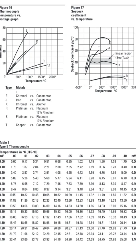
We have used hardware and software compensation to synthesize an ice-point reference. Now all we have to do is to read the digital voltmeter and convert the voltage reading to a temperature. Unfortunately, the tem-perature-versus-voltage relationship of a thermocouple is not linear. Output voltages for some popular thermocou-ples are plotted as a function of tem-perature in Figure 16. If the slope of the curve (the Seebeck coefficient) is plotted vs. temperature, as in Figure 17, it becomes quite obvious that the thermocouple is a non-linear device. A horizontal line in Figure 17 would indicate a constant α, in other words, a linear device. We notice that the slope of the type K thermocouple approaches a constant over a temp-erature range from 0° C to 1000° C. Consequently, the type K can be used with a multiplying voltmeter and an external ice point reference to obtain a moderately accurate direct readout of temperature. That is, the temperature display involves only a scale factor.

By examining the variations in Seebeck coefficient, we can easily see that using one constant scale factor would limit the temperature range of the sys-tem and restrict the syssys-tem accuracy. Better conversion accuracy can be obtained by reading the voltmeter and consulting the NIST Thermocouple Tables4_{(NIST Monograph 175 —}

see Table 3).

We could store these look-up table values in a computer, but they would consume an inordinate amount of memory. A more viable approach is to approximate the table values using a power series polynomial:

t₉₀= c₀+ c₁x + c₂x2+ c₃x3+ ... + c_nxn where

t₉₀= Temperature

x = Thermocouple Voltage

c = Polynomial coefficients unique to each thermocouple

n = Maximum order of the polynomial

Table 3 Type E Thermocouple Temperatures in °C (ITS-90) mV .00 .01 .02 .03 .04 .05 .06 .07 .08 .09 .10 mV 0.00 0.00 0.17 0.34 0.51 0.68 0.85 1.02 1.19 1.36 1.53 1.70 0.00 0.10 1.70 1.87 2.04 2.21 2.38 2.55 2.72 2.89 3.06 3.23 3.40 0.10 0.20 3.40 3.57 3.74 3.91 4.08 4.25 4.42 4.59 4.76 4.92 5.09 0.20 0.30 5.09 5.26 5.43 5.60 5.77 5.94 6.11 6.28 6.45 6.61 6.78 0.30 0.40 6.78 6.95 7.12 7.29 7.46 7.63 7.79 7.96 8.13 8.30 8.47 0.40 0.50 8.47 8.64 8.80 8.97 9.14 9.31 9.48 9.64 9.81 9.98 10.15 0.50 0.60 10.l5 10.32 10.48 10.65 10.82 10.99 11.15 11.32 11.49 11.66 11.82 0.60 0.70 11.82 11.99 12.16 12.33 12.49 12.66 12.83 12.99 13.16 13.33 13.50 0.70 0.80 13.50 13.66 13.83 14.00 14.16 14.33 14.50 14.66 14.83 15.00 15.16 0.80 0.90 15.16 15.33 15.50 15.66 15.83 16.00 16.16 16.33 16.49 16.66 16.83 0.90 1.00 16.83 l6.99 17.16 17.32 17.49 17.66 17.82 17.99 18.15 18.32 18.49 1.00 1.10 18.49 18.65 18.82 18.98 19.15 19.31 19.48 19.64 19.81 19.98 20.14 1.10 1.20 20.14 20.31 20.47 20.64 20.80 20.97 21.13 21.30 21.46 21.63 21.79 1.20 1.30 21.79 21.96 22.12 22.29 22.45 22.61 22.78 22.94 23.11 23.27 23.44 1.30 1.40 23.44 23.60 23.77 23.93 24.10 24.26 24.42 24.59 24.75 24.92 25.08 1.40 Figure 16 Thermocouple temperature vs. voltage graph Figure 17 Seebeck coefficient vs. temperature 80 60 40 20 0 _{500° 1000°} 1500° 2000° M illivo lts Temperature °C E K J R T S T Type Metals + -E Chromel vs. Constantan J Iron vs. Constantan K Chromel vs. Alumel R Platinum vs. Platinum 13% Rhodium S Platinum vs. Platinum 10% Rhodium T Copper vs. Constantan E K J R S 80 60 40 20 -500° 0° 500° 1000° 1500° T Temperature °C Seebeck Coefficient µV/°C 2000° 100 linear region (See Text)

As n increases, the accuracy of the polynomial improves. Lower order polynomials may be used over a nar-row temperature range to obtain high-er system speed. Table 4 is an example of the polynomials used in conjunction with software compensation for a data acquisition system. Rather than directly calculating the exponentials, the software is programmed to use the

nested polynomialform to save

exe-cution time. The polynomial fit rapidly degrades outside the temperature range shown in Table 4 and should not be extrapolated outside those limits. The calculation of high-order polyno-mials is a time consuming task, even for today’s high-powered micropro-cessors. As we mentioned before, we can save time by using a lower order polynomial for a smaller temperature range. In the software for one data acquisition system, the thermocouple characteristic curve is divided into eight sectors and each sector is approximated by a third-order polynomial (Figure 18).

The data acquisition system measures the output voltage, categorizes it into one of the eight sectors, and chooses the appropriate coefficients for that sector. This technique is both faster and more accurate than the higher-order polynomial.

An even faster algorithm is used in many new data acquisition systems. Using many more sectors and a series of first order equations, they can make hundreds, even thousands, of internal calculations per second.

All the foregoing procedures assume the thermocouple voltage can be measured accurately and easily; however, a quick glance at Table 5 shows us that thermocouple output voltages are very small indeed. Examine the requirements of the system voltmeter.

Table 4

NIST ITS-90 Polynomial Coefficients

Thermocouple Type Type J Type K

Temperature Range -210° C to O°C O° C to 760° C -200° C to 0° C 0° C to 500° C Error Range ± 0.05° C ± 0.04° C ± 0.04° C ±0.05° C Polynomial Order 8th order 7th order 8th order 9th order

C₀ 0 0 0 0 C₂ 1.9528268 x 10-2 _{1.978425 x 10}-2 _{2.5173462 x 10}-2 _{2.508355 x 10}-2 C₁ -1.2286185 x 10-6 _{-2.001204 x 10}-7 _{-1.1662878 x 10}-6 _{7.860106 x 10}-8 C₃ -1.0752178 x 10-9 _{1.036969 x 10}-11 _{-1.0833638 x 10}-9 _{-2.503131 x 10}-10 C₄ -5.9086933 x 10-13 _{-2.549687 x 10}-16 _{-8.9773540 v 10}-13 _{8.315270 x 10}-14 C₅ -1.7256713 x 10-16 _{3.585153 x 10}-21 _{-3.7342377 x 10}-16 _{-1.228034 x 10}-17 C₆ -2.8131513 x 10-20 _{-5.344285 x 10}-26 _{-8.6632643 x 10}-20 _{9.804036 x 10}-22 C₇ -2.3963370 x 10-24 _{5.099890 x 10}-31 _{-1.0450598 x 10}-23 _{-4.413030 x 10}-26 C₈ -8.3823321 x 10-29 _{-5.1920577 x 10}-28 _{1.057734 x 10}-30 C₉ -1.052755 x 10-35

Temperature Conversion Equation: t₉₀= c₀+ c₁x + c₂x2_{+ . . . + c}

9x9

Nested Polynomial Form (4th order example): t₉₀= c₀+ x(c₁+ x(c₂+ x(c₃+ c₄x)))

Even for the common type K thermo-couple, the voltmeter must be able to resolve 4 µV to detect a 0.1° C change. This demands both excellent resolu-tion (the more bits, the better) and measurement accuracy from the DMM. The magnitude of this signal is an open invitation for noise to creep into any system. For this reason instrument designers utilize several fundamental noise rejection tech-niques, including tree switching, normal mode filtering, integration and isolation.

Table 5

Required DVM sensitivity

Thermocouple SeebeckCoefficient DVM Sensitivity Type at 25° C (µV/°C) for 0.1° C (µV) E 61 6.1 J 52 5.2 K 40 4.0 R 6 0.6 S 6 0.6 T 41 4.1 Figure 18 Curve divided into sectors

{

Noise Rejection

Tree Switching- Tree switching is a

method of organizing the channels of a scanner into groups, each with its own main switch.

Without tree switching, every channel can contribute noise directly through its stray capacitance. With tree switch-ing, groups of parallel channel capaci-tances are in series with a single tree switch capacitance. The result is greatly reduced crosstalk in a large data acquisition system, due to the reduced interchannel capacitance (Figure 19).

Practical Thermocouple

Measurement

Analog Filter- A filter may be used

directly at the input of a voltmeter to reduce noise. It reduces interference dramatically, but causes the voltmeter to respond more slowly to step inputs (Figure 20).

Integration- Integration is an A/D

technique which essentially averages noise over a full line cycle, thus power line-related noise and its harmonics are virtually eliminated. If the integra-tion period is chosen to be less than an integer line cycle, its noise rejec-tion properties are essentially negated.

Since thermocouple circuits that cover long distances are especially susceptible to power line related noise, it is advisable to use an integrat-ing analog-to-digital converter to measure the thermocouple voltage. Integration is an especially attractive A/D technique in light of recent inno-vations have brought the cost in line with historically less expensive A/D technologies.

=

~

=

20 C HI DVM Signal + -Noise Source C _HI DVM

~

~

~

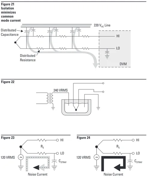
Isolation- A noise source that is common to both high and low meas-urement leads is called common mode noise. Isolated inputs help to reduce this noise as well as protect the measurement system from ground loops and transients (Figure 21). Let’s assume a thermocouple wire has been pulled through the same conduit as a 220V AC supply line. The capaci-tance between the power lines and the thermocouple lines will create an AC signal of approximately equal magni-tude on both thermocouple wires. This is not a problem in an ideal circuit, but the voltmeter is not ideal. It has some capacitance between its low terminal and safety ground (earth). Current flows through this capacitance and through the thermocouple lead resist-ance, creating a normal mode signal which appears as measurement error. This error is reduced by isolating the input terminals from safety ground with a careful design that minimizes the low-earth capacitance. Non-isolated or ground-referenced inputs (“single-ended” inputs are often ground-referenced) don’t have the ability to reject common mode noise. Instead, the common mode current flows through the low lead directly to ground, causing potentially large reading errors.

Isolated inputs are particularly useful in eliminating ground loops created when the thermocouple junction comes into direct contact with a common mode noise source. In Figure 22 we want to measure the temperature at the center of a molten metal bath that is being heated by electric current. The potential at the center of the bath is 120 VRMS. The equivalent circuit is shown in Figure 23.

Isolated inputs reject the noise current by maintaining a high impedance between LO and Earth. A non-isolated system, represented in Figure 24, completes the path to earth resulting in a ground loop. The resulting currents can be dangerously high

and can be harmful to both instrument and operator. Isolated inputs are required for making measurements with high common mode noise. Sometimes having isolated inputs isn’t enough. In Figure 23, the voltmeter inputs are floating on a 120 VRMS common mode noise source. They must withstand a peak offset of ±170 V from ground and still make accurate measurements. An isolated system with electronic FET switches typically can only handle ±12 V of offset from earth; if used in this appli-cation, the inputs would be damaged. The solution is to use commercially available external signal conditioning

Figure 21 Isolation minimizes common mode current Figure 22 Figure 23 Figure 24 Distributed Capacitance Distributed Resistance 220 V LineAC HI DVM LO

(isolation transformers and amplifiers) that buffer the inputs and reject the common mode voltage. Another easy alternative is to use a data acquisition system that can float several hundred volts.

Notice that we can also minimize the noise by minimizing R_S. We do this by using larger thermocouple wire that has a smaller series resist-ance. Also, to reduce the possibility of magnetically induced noise, the thermocouple should be twisted in a uniform manner. Thermocouple extension wires are available commer-cially in a twisted pair configuration.

240 VRMS HI LO CSTRAY RS 120 VRMS Noise Current

~

~

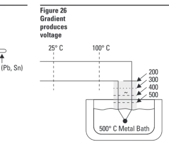
by the section of wire that contains a temperature gradient, and not neces-sarily by the junction.9For example, if we have a thermal probe located in a molten metal bath, there will be two regions that are virtually isothermal and one that has a large gradient. In Figure 26, the thermocouple junc-tion will not produce any part of the output voltage. The shaded section will be the one producing virtually the entire thermocouple output voltage. If, due to aging or annealing, the output of this thermocouple was found to be drifting, replacing only the thermocou-ple junction would not solve the prob-lem. We would have to replace the entire shaded section, since it is the source of the thermocouple voltage. Thermocouple wire obviously can’t be manufactured perfectly; there will be some defects which will cause output voltage errors. These inhomo-geneities can be especially disruptive if they occur in a region of steep temperature gradient.

Since we don’t know where an imperfection will occur within a wire, the best thing we can do is to avoid creating a steep gradient. Gradients can be reduced by using metallic sleeving or by careful placement of the thermocouple wire.

Commercial thermocouples are welded on expensive machinery using a capacitive-discharge technique to insure uniformity.

A poor weld can, of course, result in an open connection, which can be detected in a measurement situation by performing an open thermocouple check. This is a common test function available with many data loggers and data acquisition systems.

Decalibration

Decalibration is a far more serious fault condition than the open thermo-couple because it can result in temperature reading that appears to be correct. Decalibration describes the process of unintentionally altering the physical makeup of the thermocouple wire so that it no longer conforms to the NIST polynomial within specified limits. Decalibration can result from diffusion of atmospheric particles into the metal, caused by temperature extremes. It can be caused by high temperature annealing or by cold-working the metal, an effect that can occur when the wire is drawn through a conduit or strained by rough handling or vibration. Annealing can occur within the section of wire that undergoes a temperature gradient. Robert Moffat in his Gradient

Approach to Thermocouple

Thermometryexplains that the

ther-Practical Precautions

We have discussed the concepts of the reference junction, how to use a polynomial to extract absolute temper-ature data and what to look for in a data acquisition system to minimize the effects of noise. Now let’s look at the thermocouple wire itself. The polynomial curve fit relies upon the thermocouple wire being perfect; that is, it must not become decalibrated during the act of making a tempera-ture measurement. We shall now discuss some of the pitfalls of thermocouple thermometry.

Aside from the specified accuracies of the data acquisition system and its isothermal reference junction, most measurement error may be traced to one of these primary sources: 1. Poor junction connection

2. Decalibration of thermocouple wire 3. Shunt impedance and

galvanic action 4. Thermal shunting

5. Noise and leakage currents 6. Thermocouple specifications 7. Documentation

Poor Junction Connection

There are a number of acceptable ways to connect two thermocouple wires: soldering, silver-soldering, weld-ing, etc. When the thermocouple wires are soldered together, we introduce a third metal into the thermocouple circuit. As long as the temperatures on both sides of the thermocouple are the same, the solder should not introduce an error. The solder does limit the maximum temperature to which we can subject this junction (Figure 25). To reach a high measurement temper-ature, the joint must be welded. But welding is not a process to be taken lightly.5_{Overheating can degrade}

the wire, and the welding gas and the atmosphere in which the wire is welded can both diffuse into the thermocouple metal, changing its characteristics. The difficulty is com-pounded by the very different nature of the two metals being joined.

Figure 25 Soldering a thermocouple Figure 26 Gradient produces voltage Solder (Pb, Sn) Junction: Fe - Pb, Sn - C≅ Fe - C C Fe 200 25° C 100° C 300 400 500 500° C Metal Bath ~

Shunt Impedance

High temperatures can also take their toll on thermocouple wire insulators. Insulation resistance decreases expo-nentially with increasing temperature, even to the point that it creates a vir-tual junction. Assume we have a com-pletely open thermocouple operating at a high temperature (Figure 27). The leakage resistance, R_Lcan be sufficiently low to complete the circuit path and give us an improper voltage reading. Now let’s assume the thermo-couple is not open, but we are using a very long section of small diameter wire (Figure 28).

If the thermocouple wire is small, its series resistance, R_S, will be quite high and under extreme conditions R_L<< R_S.This means that the thermo-couple junction will appear to be at R_Land the output will be proportional to T₁, not T₂.

High temperatures have other detri-mental effects on thermocouple wire. The impurities and chemicals within the insulation can actually diffuse into the thermocouple metal causing the temperature-voltage dependence to deviate from the published values. When using thermocouples at high temperatures, the insulation should be chosen carefully. Atmospheric effects can be minimized by choosing the proper protective metallic or ceramic sheath.

Galvanic Action

The dyes used in some thermocouple insulation will form an electrolyte in the presence of water. This creates a galvanic action, with a resultant out-put hundreds of times greater than the Seebeck effect. Precautions should be taken to shield the thermocouple wires from all harsh atmospheres and liquids.

Thermal Shunting

No thermocouple can be made without mass. Since it takes energy to heat any mass, the thermocouple will slightly alter the temperature it was meant to measure. If the mass to be measured is small, the thermocouple must naturally be small. But a thermo-couple made with small wire is far more susceptible to the problems of contamination, annealing, strain, and shunt impedance.7To minimize these effects, thermocouple extension wire can be used.

Extension wire is commercially avail-able wire primarily intended to cover long distances between the measuring thermocouple and the voltmeter. Extension wire is made of metals hav-ing Seebeck coefficients very similar to a particular thermocouple type. It is generally larger in size so that its series resistance does not become a factor when traversing long distances. It can also be pulled more readily through conduit than very small thermocouple wire. It generally is specified over a much lower tempera-ture range than premium-grade ther-mocouple wire. In addition to offering a practical size advantage, extension wire is less expensive than standard thermocouple wire. This is especially true in the case of platinum-based thermocouples.

Since the extension wire is specified over a narrower temperature range and it is more likely to receive mechanical stress, the temperature gradient across the extension wire should be kept to a minimum. This, according to the gradient theory, assures that virtually none of the output signal will be affected by the extension wire.

Noise- We have already discussed

the line-related noise as it pertains to the data acquisition system. The techniques of integration, tree switch-ing and isolation serve to cancel most line-related interference. Broadband noise can be rejected with an analog filter.

The one type of noise the data acquisition system cannot reject is a DC offset caused by a DC leakage current in the system. While it is less common to see DC leakage currents of sufficient magnitude to cause appreciable error, the possibility of their presence should be noted and prevented, especially if the thermo-couple wire is very small and the related series impedance is high.

Figure 27 Leakage resistance Figure 28 Virtual junction To DVM R_L (Open) _R S RS RS RS To DVM RL T1 T₂

Event Record- The first diagnostic is not a test at all, but a recording of all pertinent events that could even remotely affect the measurements. An example is:

Figure 29

March 18 Event Record

10:43 Power failure

10:47 System power returned

11:05 Changed M821 to

type K thermocouple

13:51 New data acquisition program

16:07 M821 appears to be bad reading

We look at our program listing and find that measurand #M821 uses a type J thermocouple and that our new data acquisition program interprets it as type J. But from the event record, apparently thermocouple #M821 was changed to a type K, and the change was not entered into the program. While most anomalies are not discov-ered this easily, the event record can provide valuable insight into the reason for an unexplained change in a system measurement. This is espe-cially true in a system configured to measure hundreds of data points. Since channel numbers invariably

change, data should be categorized by measurand, not just channel number.10

Information about any given measur-and, such as transducer type, output voltage, typical value, and location can be maintained in a data file. This can be done under PC control or simply by filling out a preprinted form. No matter how the data is maintained, the importance of a concise system should not be underestimated, especially at the outset of a complex data gathering project.

Diagnostics

Most of the sources of error that we have mentioned are aggravated by using the thermocouple near its tem-perature limits. These conditions will be encountered infrequently in most applications. But what about the situa-tion where we are using small thermo-couples in a harsh atmosphere at high temperatures? How can we tell when the thermocouple is producing erro-neous results? We need to develop a reliable set of diagnostic procedures. Through the use of diagnostic techniques, R.P. Reed has developed an excellent system for detecting a faulty thermocouple and data chan-nels.10_{Three components of this}

system are the event record, the zone box test and the thermocouple resistance history.

Wire Calibration

Thermocouple wire is manufactured to a certain specification signifying its conformance with the NIST tables. The specification can sometimes be enhanced by calibrating the wire (testing it at known temperatures). Consecutive pieces of wire on a con-tinuous spool will generally track each other more closely than the specified tolerance, although their output volt-ages may be slightly removed from the center of the absolute specification. If the wire is calibrated in an effort to improve its fundamental specifica-tions, it becomes even more impera-tive that all of the aforementioned conditions be heeded in order to avoid decalibration.

Documentation

It may seem incongruous to speak of documentation as being a source of voltage measurement error, but the fact is that thermocouple systems, by their very ease of use, invite a large number of data points. The sheer mag-nitude of the data can become quite unwieldy. When a large amount of data is taken, there is an increased proba-bility of error due to mislabeling of lines, using the wrong NIST curve, etc.

Zone Box Test- The zone box is an isothermal terminal block with a known temperature used in place of an ice bath reference. If we temporari-ly short-circuit the thermocouple directly at the zone box, the system should read a temperature very close to that of the zone box, i.e., close to room temperature (Figure 30). If the thermocouple lead resistance is much greater than the shunting resist-ance, the copper wire shunt forces V = 0. In the normal unshorted case, we want to measure T_J, and the system reads:

V = α(T_J– T_REF)

But, for the functional test, we have shorted the terminals so that V = 0. The indicated temperature TJ is thus: 0 = α(T_J– T_REF)

T_J= T_REF

Thus, for a DVM reading of V = 0, the system will indicate the zone box temperature. First we observe the temperature T_J(forced to be different from T_REF), then we short the thermo-couple with a copper wire and make sure that the system indicates the zone box temperature instead of T_J. This simple test verifies that the controller, scanner, voltmeter and zone box compensation are all operating correctly. In fact, this simple procedure tests everything but the thermocouple wire itself.

Thermocouple Resistance- A

sud-den change in the resistance of a ther-mocouple circuit can act as a warning indicator. If we plot resistance vs. time for each set of thermocouple wires, we can immediately spot a sudden resistance change, which could be an indication of an open wire, a wire shorted due to insulation failure, changes due to vibration fatigue or one of many failure mechanisms. For example, assume we have the thermocouple measurement shown in Figure 31.

We want to measure the temperature profile of an underground seam of coal that has been ignited. The wire passes through a high temperature region, into a cooler region. Suddenly, the temperature we measure rises from 300° C to 1200° C. Has the burning section of the coal seam migrated to a different location, or has the thermocouple insulation failed, thus causing a short circuit between the two wires at the point of a hot spot?

If we have a continuous history of the thermocouple wire resistance, we can deduce what has actually happened (Figure 32). Figure 30 Shorting the thermocouples at the terminals Figure 32 Thermocouple resistance vs. time Figure 31 Burning coal seam C TREF HI LO + -v Cu Cu Voltmeter TJ

Copper Wire Short Fe Cu Cu Zone Box Isothermal Block T1 T = 1200° C To Data Acquisition System T = 300° C Resi st ance Time t1

The resistance of the thermocouple will naturally change with time as the resistivity of the wire changes due to varying temperatures. But a sudden change in resistance is an indication that something is wrong. In this case, the resistance has dropped abruptly, indicating that the insulation has failed, effectively shortening the thermocouple loop (Figure 33). The new junction will measure temperature T_S, not T₁. The resistance measurement has given us additional information to help interpret the physical phenomenon that has occurred. This failure would not have been detected by a standard open-thermocouple check.

Measuring Resistance - We have

casually mentioned checking the resistance of the thermocouple wire, as if it were a straightforward measurement. But keep in mind that when the thermocouple is producing a voltage, this voltage can cause a large resistance measurement error. Measuring the resistance of a thermo-couple is akin to measuring the internal resistance of a battery. We can attack this problem with a technique known as offset compensated ohms

measurement.

As the name implies, the data acquisition unit first measures the thermocouple offset voltage without the ohms current source applied. Then the ohms current source is switched on and the voltage across the resistance is again measured. The instrument firmware compensates for the offset voltage of the thermocouple and calculates the actual thermo-couple source resistance.

Special Thermocouples- Under

extreme conditions, we can even use diagnostic thermocouple circuit configurations. Tip-branched and

leg-branchedthermocouples are

four-wire thermocouple circuits that allow redundant measurement of tempera-ture, noise voltage and resistance for checking wire integrity (Figure 34). Their respective merits are discussed in detail in Bibliography 8.

Only severe thermocouple applica-tions require such extensive diagnos-tics, but it is comforting to know that there are procedures that can be used to verify the integrity of an important thermocouple measurement.

Summary

In summary, the integrity of a thermo-couple system may be improved by following these precautions:

●_{Use the largest wire possible that}

will not shunt heat away from the measurement area.

●_{If small wire is required, use it only}

in the region of the measurement and use extension wire for the region with no temperature gradient.

●_{Avoid mechanical stress and}

vibra-tion, which could strain the wires.

●_{When using long thermocouple}

wires, use shielded, twisted pair extension wire.

●_{Avoid steep temperature gradients.} ●_{Try to use the thermocouple wire}

well within its temperature rating.

●_{Use an integrating A/D converter}

with high resolution and good accuracy.

●_{Use isolated inputs with ample}

offset capability.

●_{Use the proper sheathing material in}

hostile environments to protect the thermocouple wire.

●_{Use extension wire only at low}

temperatures and only in regions of small gradients.

●_{Keep an event log and a continuous}

record of thermocouple resistance.

Figure 33 Cause of the resistance change Figure 34 TS T1

Short Leg-Branched Thermocouple

History

The same year that Seebeck made his discovery about thermoelectricity, Sir Humphrey Davy announced that the resistivity of metals showed a marked temperature dependence. Fifty years later, Sir William Siemens proffered the use of platinum as the element in a resistance thermometer. His choice proved most propitious, as platinum is used to this day as the primary element in all high-accuracy resistance thermometers. In fact, the platinum resistance temperature detector, or PRTD, is used today as an interpola-tion standard from the triple point of equilibrium hydrogen (–259.3467° C) to the freezing point of silver (961.78° C). Platinum is especially suited to this purpose, as it can withstand high temperatures while maintaining excellent stability. As a noble metal, it shows limited susceptibility to contamination.

The classical resistance temperature detector (RTD) construction using platinum was proposed by C.H. Meyers in 1932.12_{He wound a helical}

coil of platinum on a crossed mica web and mounted the assembly inside a glass tube. This construction minimized strain on the wire while maximizing resistance (Figure 35). Although this construction produces a very stable element, the thermal contact between the platinum and the measured point is quite poor. This results in a slow thermal response time. The fragility of the structure limits its use today primarily to that of a laboratory standard.

Another laboratory standard has taken the place of the Meyer’s design. This is the bird-cage element proposed by Evans and Burns.16The platinum element remains largely unsupported, which allows it to move freely when expanded or contracted by temperature variations (Figure 36).

Strain-induced resistance changes caused by time and temperature are thus minimized and the bird-cage becomes the ultimate laboratory standard. Due to the unsupported structure and subsequent susceptibili-ty to vibration, this configuration is still a bit too fragile for industrial environments.

A more rugged construction technique is shown in Figure 37. The platinum wire is bifilar wound on a glass or ceramic bobbin. The bifilar winding reduces the effective enclosed area of the coil to minimize magnetic pickup and its related noise. Once the wire is wound onto the bobbin, the assembly is then sealed with a coating of molten glass. The sealing process assures that the RTD will maintain its integrity

under extreme vibration, but it also limits the expansion of the platinum metal at high temperatures. Unless the coefficients of expansion of the platinum and the bobbin match per-fectly, stress will be placed on the wire as the temperature changes, resulting in a strain-induced resistance change. This may result in a permanent change in the resistance of the wire.

There are partially supported versions of the RTD which offer a compromise between the bird-cage approach and the sealed helix. One such approach uses a platinum helix threaded through a ceramic cylinder and affixed via glass-frit. These devices will main-tain excellent stability in moderately rugged vibrational applications.

The RTD

Sealed Bifilar Winding

Helical RTD

Metal Film RTD’s

In the newest construction technique, a platinum or metal-glass slurry film is deposited or screened onto a small flat ceramic substrate, etched with a laser-trimming system, and sealed. The film RTD offers substantial reduction in assembly time and has the further advantage of increased resistance for a given size. Due to the manufacturing technology, the device size itself is small, which means it can respond quickly to step changes in tempera-ture. Film RTD’s are less stable than their wire-wound counterparts, but they are more popular because of their decided advantages in size, production cost and ruggedness.

Metals- All metals produce a positive

change in resistance for a positive change in temperature. This, of course, is the main function of an RTD. As we shall soon see, system error is minimized when the nominal value of the RTD resistance is large. This implies a metal wire with a high resistivity. The lower the resistivity of the metal, the more material we will have to use.

Table 6 lists the resistivities of common RTD materials.

Because of their lower resistivities, gold and silver are rarely used as RTD elements. Tungsten has a relatively high resistivity, but is reserved for very high temperature applications because it is extremely brittle and difficult to work.

Copper is used occasionally as an RTD element. Its low resistivity forces the element to be longer than a platinum element, but its linearity and very low cost make it an economical alternative. Its upper temperature limit is only about 120° C.

The most common RTD’s are made of either platinum, nickel, or nickel alloys. The economical nickel deriva-tive wires are used over a limited temperature range. They are quite non-linear and tend to drift with time. For measurement integrity, platinum is the obvious choice.

Resistance Measurement

The common values of resistance for a platinum RTD range from 10 ohms for the bird-cage model to several thousand ohms for the film RTD. The single most common value is 100 ohms at 0° C. The DIN 43760 standard temperature coefficient of platinum wire is α= .00385. For a 100 ohm wire this corresponds to +0.385 Ω/°C at 0° C. This value for αis actually the

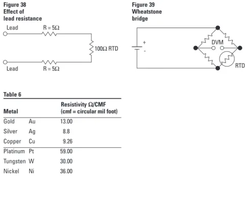
average slope from 0° C to 100° C. The more chemically pure platinum wire used in platinum resistance standards has an αof +.00392 ohms/ohm/° C. Both the slope and the absolute value are small numbers, especially when we consider the fact that the measure-ment wires leading to the sensor may be several ohms or even tens of ohms. A small lead impedance can contribute a significant error to our temperature measurement (Figure 38).

A 10 ohm lead impedance implies 10/.385 ≅26° C error in our measure-ment. Even the temperature coeffi-cient of the lead wire can contribute a measurable error. The classical method of avoiding this problem has been the use of a bridge (Figure 39).

Figure 38 Effect of lead resistance

Table 6

Resistivity ΩΩ/CMF Metal (cmf = circular mil foot)

Gold Au 13.00 Silver Ag 8.8 Copper Cu 9.26 Platinum Pt 59.00 Tungsten W 30.00 Nickel Ni 36.00 Figure 39 Wheatstone bridge 100ΩRTD R = 5Ω Lead Lead R = 5Ω DVM RTD +

-The bridge output voltage is an indi-rect indication of the RTD resistance. The bridge requires four connection wires, an external source, and three resistors that have a zero temperature coefficient. To avoid subjecting the three bridge-completion resistors to the same temperature as the RTD, the RTD is separated from the bridge by a pair of extension wires (Figure 40). These extension wires recreate the problem that we had initially: The impedance of the extension wires affects the temperature reading. This effect can be minimized by using a

three-wire bridge configuration

(Figure 41).

If wires A and B are perfectly matched in length, their impedance effects will cancel because each is in an opposite leg of the bridge. The third wire, C, acts as a sense lead and carries no current.

The Wheatstone bridge shown in Figure 41 creates a non-linear relation-ship between resistance change and bridge output voltage change. This compounds the already non-linear temperature-resistance characteristic of the RTD by requiring an additional equation to convert bridge output voltage to equivalent RTD impedance.

4-Wire Ohms- The technique of using

a current source along with a remotely sensed digital voltmeter alleviates many problems associated with the bridge. Since no current flows through the voltage sense leads, there is no IR drop in these leads and thus no lead resistance error in the measurement. The output voltage read by the DVM is directly proportional to RTD resistance, so only one conversion equation is necessary. The three bridge-completion resistors are replaced by one reference resistor. The digital voltmeter measures only the voltage dropped across the RTD and is insensitive to the length of the lead wires (Figure 42).

The one disadvantage of using 4-wire ohms is that we need one more exten-sion wire than the 3-wire bridge. This is a small price to pay if we are at all concerned with the accuracy of the temperature measurement.

Resistance to

Temperature Conversion

The RTD is a more linear device than the thermocouple, but it still requires curve-fitting. The Callendar-Van Dusen equation has been used for years to approximate the RTD curve.11, 13

R_T=R₀+R₀α T–δ -1 -β -1 Where: R_T= resistance at temperature T R₀= resistance at T = 0° C α = temperature coefficient at T = 0° C (typically + 0.00392Ω/Ω/° C)

δ = 1.49 (typical value for .00392 platinum)

β = 0 T > 0 0.11 (typical) T < 0 Figure 40 Figure 42 4-Wire Ohms Measurement Figure 41 3-Wire Bridge DVM RTD + -DVM A C B 100ΩRTD + -DVM i = 0 i = 0 i

( )

[

]

( )

( )

( )

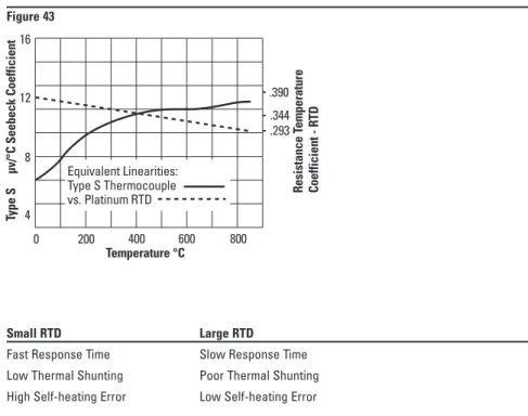
The exact values for coefficients α, δ and βare determined by testing the RTD at four temperatures and solving the resultant equations. This familiar equation was replaced in 1968 by a 20th order polynomial in order to provide a more accurate curve fit. The plot of this equation shows the RTD to be a more linear device than the thermocouple (Figure 43).

Practical Precautions

The same practical precautions that apply to thermocouples also apply to RTD’s, i.e., use shields and twisted-pair wire, use proper sheathing, avoid stress and steep-gradients, use large extension wire, keep good documenta-tion and use an integrating DMM. In addition, the following precautions should be observed.

Construction- Due to its

construc-tion, the RTD is somewhat more fragile than the thermocouple, and precautions must be taken to protect it.

Self-Heating- Unlike the

thermo-couple, the RTD is not self-powered. A current must be passed through the device to provide a voltage that can be measured. The current causes Joule (I2R) heating within the RTD, chang-ing its temperature. This self-heatchang-ing appears as a measurement error. Consequently, attention must be paid

to the magnitude of the measurement current supplied by the ohmmeter. A typical value for self-heating error is ½° C per milliwatt in free air. Obviously, an RTD immersed in a thermally conductive medium will distribute its Joule heat to the medium and the error due to self-heating will be smaller. The same RTD that rises 1° C per milliwatt in free air will rise only 1/10° C per milliwatt in air which is flowing at the rate of one meter per second.6

To reduce self-heating errors, use the minimum ohms measurement current that will still give the resolution you

Figure 43 12 8 4 0 200 400 600 Temperature °C .390 .344 .293 Ty pe S µv/°C Seebeck Coefficient Resi st ance T e m per at ur e C o e ffic ie n t - R T D 800 16 Equivalent Linearities: Type S Thermocouple vs. Platinum RTD

require, and use the largest RTD you can that will still give good response time. Obviously, there are compromises to be considered.

Thermal Shunting- Thermal

shunting is the act of altering the measurement temperature by inserting a measurement transducer. Thermal shunting is more a problem with RTD’s than with thermocouples, as the physical bulk of an RTD is greater than that of a thermocouple.

Thermal EMF- The

platinum-to-copper connection that is made when the RTD is measured can cause a thermal offset voltage. The offset-compensated ohms technique can be used to eliminate this effect.

Small RTD Large RTD

Fast Response Time Slow Response Time

Low Thermal Shunting Poor Thermal Shunting

Like the RTD, the thermistor is also a temperature-sensitive resistor. While the thermocouple is the most versatile temperature transducer and the PRTD is the most stable, the word that best describes the thermistor is sensitive. Of the three major categories of sensors, the thermistor exhibits by far the largest parameter change with temperature.

Thermistors are generally composed of semiconductor materials. Although positive temperature coefficient units are available, most thermistors have a negative temperature coefficient (TC); that is, their resistance decreases with increasing temperature. The negative TC can be as large as several percent per degree C, allowing the thermistor circuit to detect minute changes in temperature which could not be observed with an RTD or thermo-couple circuit.

The price we pay for this increased sensitivity is loss of linearity. The thermistor is an extremely non-linear device which is highly dependent upon process parameters. Consequently, manufacturers have not standardized thermistor curves to the extent that RTD and thermocouple curves have been standardized (Figure 44). An individual thermistor curve can be very closely approximated through use of the Steinhart-Hart equation:18 1

= A + B(ln R) + C (ln R)3

T where: T = kelvins

R = Resistance of the thermistor A,B,C = curve-fitting constants A, B, and C are found by selecting three data points on the published data curve and solving the three simultaneous equations. When the data points are chosen to span no more than 100° C within the nominal center of the thermistor’s temperature range, this equation approaches a rather remarkable ±.02° C curve fit.

The Thermistor

Somewhat faster computer execution time is achieved through a simpler equation:

1 T =

(ln R) – A -C

where A, B, and C are again found by selecting three (R,T) data points and solving the three resultant simultane-ous equations. This equation must be applied over a narrower temperature range in order to approach the accura-cy of the Steinhart-Hart equation.

Measurement

The high resistivity of the thermistor affords it a distinct measurement advantage. The four-wire resistance measurement may not be required as it is with RTD’s. For example, a common thermistor value is 5000Ωat 25° C. With a typical TC of 4%/° C, a measurement lead resistance of 10Ω produces only .05° C error. This error is a factor of 500 times less than the equivalent RTD error.

Disadvantages- Because they are

semiconductors, thermistors are more susceptible to permanent decali-bration at high temperatures than are RTD’s or thermocouples. The use of thermistors is generally limited to a few hundred degrees Celsius, and manufacturers warn that extended exposures even well below maximum operating limits will cause the thermistor to drift out of its specified tolerance.

Thermistors can be made very small which means they will respond quickly to temperature changes. It also means that their small thermal mass makes them especially susceptible to self-heating errors. Thermistors are a good deal more fragile than RTD’s or thermocouples and they must be carefully mounted to avoid crushing or bond separation.

An innovation in thermometry is the integrated circuit temperature transducer. These are available in both voltage and current-output configurations. Both supply an output that is linearly proportional to absolute temperature. Typical values are 1 µA/K and 10 mV/K F (Figure 45). Some integrated sensors even represent temperature in a digital output format that can be read directly by a microprocessor. Except that they offer a very linear output with temperature, these IC sensors share all the disadvantages of thermistors. They are semiconductor devices and thus have a limited tem-perature range. The same problems of self-heating and fragility are evident and they require an external power source.

These devices provide a convenient way to produce an easy-to-read output that is proportional to temperature. Such a need arises in thermocouple reference junction hardware, and in fact these devices are increasingly used for thermocouple compensation.

Monolithic Linear

Temperature Sensor

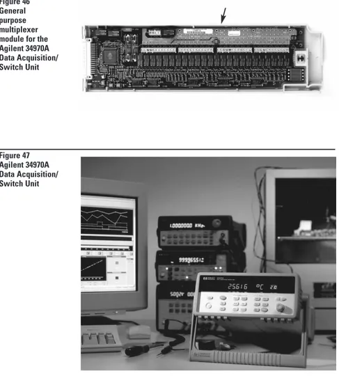
Figure 46 shows a practical method of implementing a thermocouple refer-ence junction. The arrow points to an IC sensor which is used to perform software thermocouple compensation. Conversion routines built into the Agilent 34970A firmware accept B, E, J, K, N, R, S and T type thermocouples, 2.2kΩ, 5kΩand 10kΩthermistors, as well as a wide range of RTD’s. Results are displayed directly in degrees C, F or kelvins. The Agilent 34970A data acquisition system incorporates all of the desirable features mentioned in this application note:

●_{Internal 6½ digit DMM}

●_{Integrating A/D for noise rejection} ●_{Low-thermal scanning with built-in}

thermocouple reference junctions

●_{Open thermocouple check} ●_{Built-in thermocouple, thermistor,}

and RTD linearization routines with ITS-90 conformity

●_{Four-wire Ohms function with}

offset compensation

●_{Isolated inputs that float up to 300 V}

The Agilent 34970A comes standard with RS-232 and GPIB interfaces, 50,000 readings of non-volatile memory for stand-alone data logging, and Agilent Benchlink Data Logger software for easy PC-based testing. Plus, its flexible three-slot construc-tion makes it easy to add channels for changing applications.

The Measurement System

Figure 46 General purpose multiplexer module for the Agilent 34970A Data Acquisition/ Switch Unit Figure 47 Agilent 34970A Data Acquisition/ Switch Unit

The Agilent DAC1000 data acquisition and control system (Figure 48), another example solution, provides high-speed temperature measurements where point count is high. When configured for temperature measurements, it consists of:

●_{E1419A scanning}

analog-to-digital converter (ADC) module with 64 channels that can be configured for temperature measurements. Scanning rate is 56,000 channels/s. Several hundred channel configura-tions are possible with multiple modules.

●_{Signal conditioning plug-on (SCP)}

that rides piggy-back on the ADC module provides input for thermocouples.

●_{External terminal block with}

built-in thermocouple reference junction and terminal connections to the application.

●_{Four-wire Ohms SCP with offset}

compensation for RTD and thermistor measurements.

●_{Built-in engineering unit conversions}

for thermocouple, thermistor, and RTD measurements.

This VXI-based system offers much more than temperature measurements. It provides a wide variety of analog/ digital input and output capability required by designers of electro-mechanical products and manufactur-ers needing stringent monitoring and control of physical processes. The DAC1000 is a recommended configura-tion consisting of the E1419A, 6-slot VXI mainframe, GPIB interfaces, and Agilent VEE for the PC. Agilent VEE, a powerful time-saving graphical pro-gramming language, is programmed by connecting a few icons or objects resembling a block diagram.

Figure 48 Agilent DAC1000 System

Agilent VEE provides data collection, test reporting and a friendly graphical user interface.

Agilent also offers other VXI-based solutions for temperature measure-ments. Product choices range from small compact systems for portable or remote operation to high-speed scanning systems that also provide advanced control and analysis capabilities.

Reliable temperature measurements require a great deal of care in both selecting and using the transducer, as well as choosing the right measure-ment system. With proper precautions observed for self-heating, thermal shunting, transducer decalibration, specifications and noise reduction, even the most complex temperature monitoring project will produce repeatable, reliable data. Today’s data acquisition system assumes a great deal of this burden, allowing us to concentrate on meaningful test results.